PERFORM: A Metric for Evaluating Autonomous System Performance in Marine Testbed Environments Using Interval Type-2 Fuzzy Logic

Abstract

Trust and confidence in autonomous behavior is required to send autonomous vehicles into operational missions. The authors introduce the Performance Evaluation and Review Framework Of Robotic Missions (PERFORM), a framework to enable a rigorous and replicable autonomy test environment, thereby filling the void between that of merely simulating autonomy and that of completing true field missions. A generic architecture for defining the missions under test is proposed and a unique Interval Type-2 Fuzzy Logic approach is used as the foundation for the mathematically rigorous autonomy evaluation framework. The test environment is designed to aid in (1) new technology development (i.e., providing direct comparisons and quantitative evaluations between autonomy algorithms), (2) the validation of the performance of specific autonomous platforms, and (3) the selection of the appropriate robotic platform(s) for a given mission type (e.g., for surveying, surveillance, search and rescue). Three case studies are presented to apply the metric to various test scenarios. Results demonstrate the flexibility of the technique with the ability to tailor tests to the user’s design requirements accounting for different priorities related to acceptable risks and goals of a given mission.

1. Introduction

The potential impact of autonomous (self-driving) vehicles in the ocean domain is undisputed. From exploring the more than 90% of the ocean environment that remains a mystery, to increasing data collection efficiency and cost effectiveness, to shipping and minimizing human risk in hazardous environments, autonomous marine vehicles serve scientific, commercial, and military interests. To transition these autonomous systems into operational missions, however, a quantifiable level of trust and confidence in robot actions requires validation [1,2]. Current research still primarily consists of simulations and proof-of-concept vehicles tested only in controlled laboratory or field environments due to the lack of reliable testing of autonomous decision-making [1,3,4,5]. The existing gap between technological advancement and the effective test and evaluation of these systems must be bridged to make autonomous vehicles increasingly practical for field use and not simply for an academic exercise [6,7].

Standard test and evaluation techniques, such as design of experiments and Monte Carlo analysis are unusable due to the excessive number of variables inherent to an autonomous system [8]. One technique developed by the Johns Hopkins Applied Physics Laboratory (APL) uses modeling and simulation to perform many iterations of particular scenarios and then form scores to provide some means for evaluating a statistically large number of runs. This tool, referred to as the Range Adversarial Planning Tool (RAPT), searches for boundaries in capabilities to identify the most critical tests for test range operations [6]. Other work has been done with developing methods using model-checking, finite state machines, and process algebras, but these techniques require a model that completely describes the autonomy [6]. Due to proprietary intellectual property with software and the complex nature of autonomous systems, these modeling strategies have limited applicable use [6,7]. Additionally, these strategies test the robustness of the software but do not give information about how the system will perform while executing the mission (e.g., whether the vehicle will navigate to the left or right of an obstacle) [9]. Oftentimes, new issues arise when moving from a simulation environment to an experimental platform, necessitating experimental testing as a critical component of the autonomy validation process.

Current experimental test procedures for autonomous vehicles are usually conducted on a case-by-case basis with limited mathematical rigor [7,10] and a lack of agreed upon standards and definitions for autonomous systems and related performance metrics [11,12]. Autonomous ground vehicle companies resort to driving millions of miles to perform validation tests, which is generally economically impractical [13,14,15]. Some strategies focus on autonomy level opposed to mission performance such as in the Autonomy Levels for Unmanned Systems (ALFUS) framework [10,16] and the US Army Mission Performance Potential (MPP) framework [17]. These techniques predict expected performance for a mission set and level of autonomy but it does not directly compare the performances of varying types of autonomy algorithms, nor does it provide a direct measure of vehicle performance for individual iterations of a given mission scenario.

Other test range methods have been developed in response to ground vehicle competitions such as the DARPA Grand Challenge [18,19]. These methods have applied a Type-1 Fuzzy Inference System (T1-FL) using an analytic hierarchy process (AHP) for weight distribution. T1-FL systems, however, do not take into account additional uncertainty in its given membership functions and, therefore, have limited capabilities in minimizing the effects of such uncertainties [20]. These uncertainties originate from such sources as (but not limited to) noisy measurements, the chosen linguistic terms, and the user-defined rule-base, among other variables.

The authors introduce the Performance Evaluation and Review Framework Of Robotic Missions (PERFORM), a framework with which to enable a rigorous and replicable autonomy test environment while limiting test redundancy and reducing the number of live test missions to that of a representative subset of scenarios (as determined by the user), thereby filling the void between that of merely simulating autonomy and that of completing true field missions. This environment enables (1) new technology development (i.e., providing direct comparisons and quantitative evaluations of varying autonomy algorithms), (2) the validation of the performance of specific autonomous platforms, and (3) the selection of the appropriate robotic platform(s) for a given mission type (e.g., for surveying, surveillance, search and rescue). PERFORM uses Artificial Intelligence (AI) to provide a quantified assessment of autonomous system capabilities in this testbed environment. With the use of a Type-2 Fuzzy Logic (T2-FL) system approach, this technique takes into account internal and external uncertainties (e.g., obstacles, sensor noise, and vehicle mobility). The authors use Interval Type-2 Fuzzy Logic (IT2-FL) specifically, as it is the most widely used and computationally efficient of the T2 subsets [21,22,23]. IT2-FL systems are capable of identifying and representing model uncertainty in the dynamic platform and platform environment, as well as in modeling on-board sensor measurements [21,24,25]. Designed as a Multi-Input Single-Output (MISO) system interface, the final output of the proposed AI-based (via IT2-FL) autonomy evaluation framework is a numerical performance score, which provides a high-level external view of the autonomous system with which to measure and validate system proficiency (with respect to user-specified mission tasks) and to predict overall autonomous vehicle behavior.

2. Materials and Methods

2.1. Mission Architecture

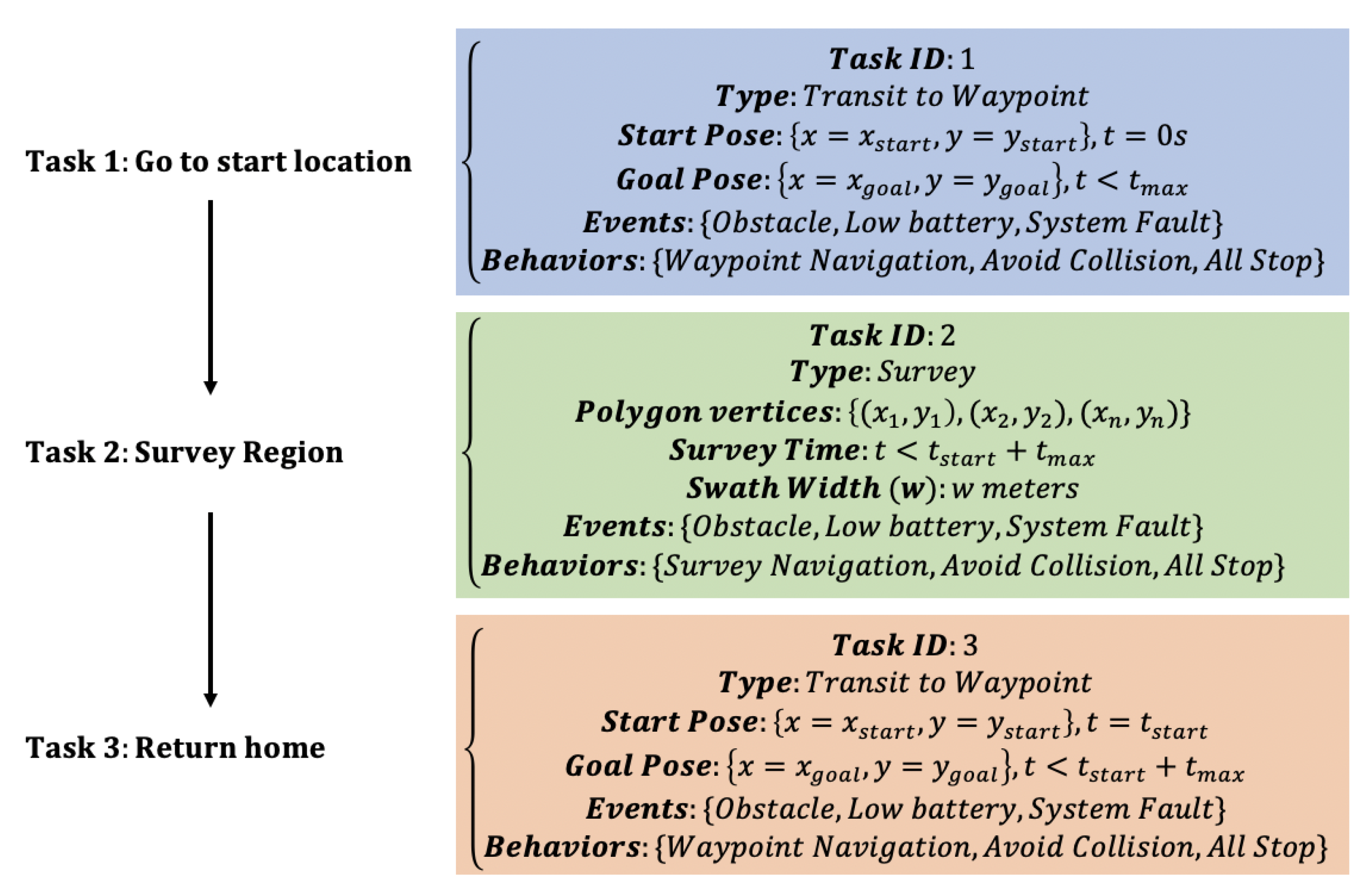
For the purpose of generalizing the autonomy evaluation procedure, a generic architecture for defining the test missions is proposed. The authors maintain that any autonomous mission may be subdivided into a set of generic tasks that autonomous missions often incorporate (e.g., transit, conduct survey, station keeping, etc.). Each task may be divided into generic subtasks (for the remaining document, task will refer to both tasks and subtasks). These tasks are separated by time and order via the mission-scripted programming but also by events that represent time-based changes in the environment (e.g., a newly discovered obstacle, a sudden change in sea state, etc.) or within the autonomous platform itself (e.g., low battery, faulty on-board sensor, etc.). Depending upon how/when these events occur during the tasks being performed, specific mission behaviors should (or must) take place in order to complete a specific task (or mission) or to prevent catastrophic system failure. In other words, behaviors consist of actions and/or reactions conducted by the autonomous vehicle during the execution of a task to aid in completion of the task. An important aspect of decomposing a mission into tasks and events is that at the lowest level of the decomposition, there could be significant overlap of tasks and reactions to events for a wide variety of missions. This enables one to make inferences about future autonomous capability from the evaluation performed in this environment for a set of canonical missions. Flexibility in mission definitions to capture a range of operational scenarios (as opposed to testing individual scenarios) during evaluation is highly desirable [26]. Describing a mission with tasks and associated events form the foundations for creating the corresponding scenarios and metrics.

In the proposed architecture, a mission (M) is defined as a set of tasks that must be completed to realize a specific goal or goals. Tasks (T) are a set of data structures that define quantifiable starting and ending states (as a function of time and space) and that can be combined with other tasks to realize a mission goal. Tasks should be described through simple language (e.g., travel to a desired waypoint), and they are conditionally dependent within a specific mission such that relations between the order of tasks can be represented as a directed graph. Events (E) are defined as a set of possible time-based changes (both internal and external to the given autonomous vehicle) that occur during and/or as a result of a specific task. Behaviors (B) are defined as the actions necessary to perform a given task (e.g., avoid known obstacle, no event occurring, etc.) or occur in response to an event (e.g., avoid a new obstacle, perform station keeping, etc.). Example parameters used for performance evaluation may include elements such as the vehicle’s total time and distance traveled to complete a task, the closest point of approach (CPA), and the total energy consumed.

Scenarios become instances of a given mission and are defined such that S denotes a space of all possible scenarios that can be“realized” with respect to the mission and the platform being used to accomplish the mission. Each element S_i ∈ S is selected by choosing values for a set of scenario parameters that are derived from key aspects of the mission description. Scenario parameters may encompass items such as survey areas (box size and location), launch/recovery points, time of day, and starting battery charge. A metric function, $\mu$, maps elements of the scenario space $S_i$ to ℜ values:

$$\forall S_{ik}\in S_i\exists \mu :\mu \left(S_{ik}\right)\in \Re$$

(1)

thereby combining many aspects for evaluating performance of the autonomous vehicle as it reacts to events and accomplishes tasks as it executes the scenario. Essentially, this metric produces a score for every scenario (a realized instance of the mission). In set notation, the mission space with the associated T, E, B, and S may be represented as follows:

$$M\left(S_i\right)=\left\{\begin{array}{c}{M}_{1i}=\left\{T_{11}(t,x,y,z,B,E),T_{12}(t,x,y,z,B,E),...,T_{1n}(t,x,y,z,B,E)\right\}\hfill \\ M_{2i}=\left\{T_{21}(t,x,y,z,B,E),T_{22}(t,x,y,z,B,E),...,T_{2n}(t,x,y,z,B,E)\right\}\hfill \\ ⋮\hfill \\ M_{mi}=\left\{T_{m1}(t,x,y,z,B,E),T_{m2}(t,x,y,z,B,E),...,T_{mn}(t,x,y,z,B,E)\right\}\hfill \end{array}\right.$$

(2)

where m, n, and i are mission number, task number, and scenario number, respectively. Figure 1 gives an overview of an example Autonomous Surface Vehicle (ASV) seafloor mapping mission with the proposed architecture.

By representing a mission with this framework, set operations may then be used to compare various generic missions and tasks with the intention of limiting test redundancy and reducing the number of test missions to that of the most critical scenarios. The main goal here is to alleviate the need to determine the exhaustive list of all possible scenarios and combinations of mission tasks, events, and behaviors for which the performance of the vehicle autonomy must be tested against. Instead, this mission framework provides an analysis platform with which to test/observe platform autonomy and which is fully modular, versatile, and scalable.

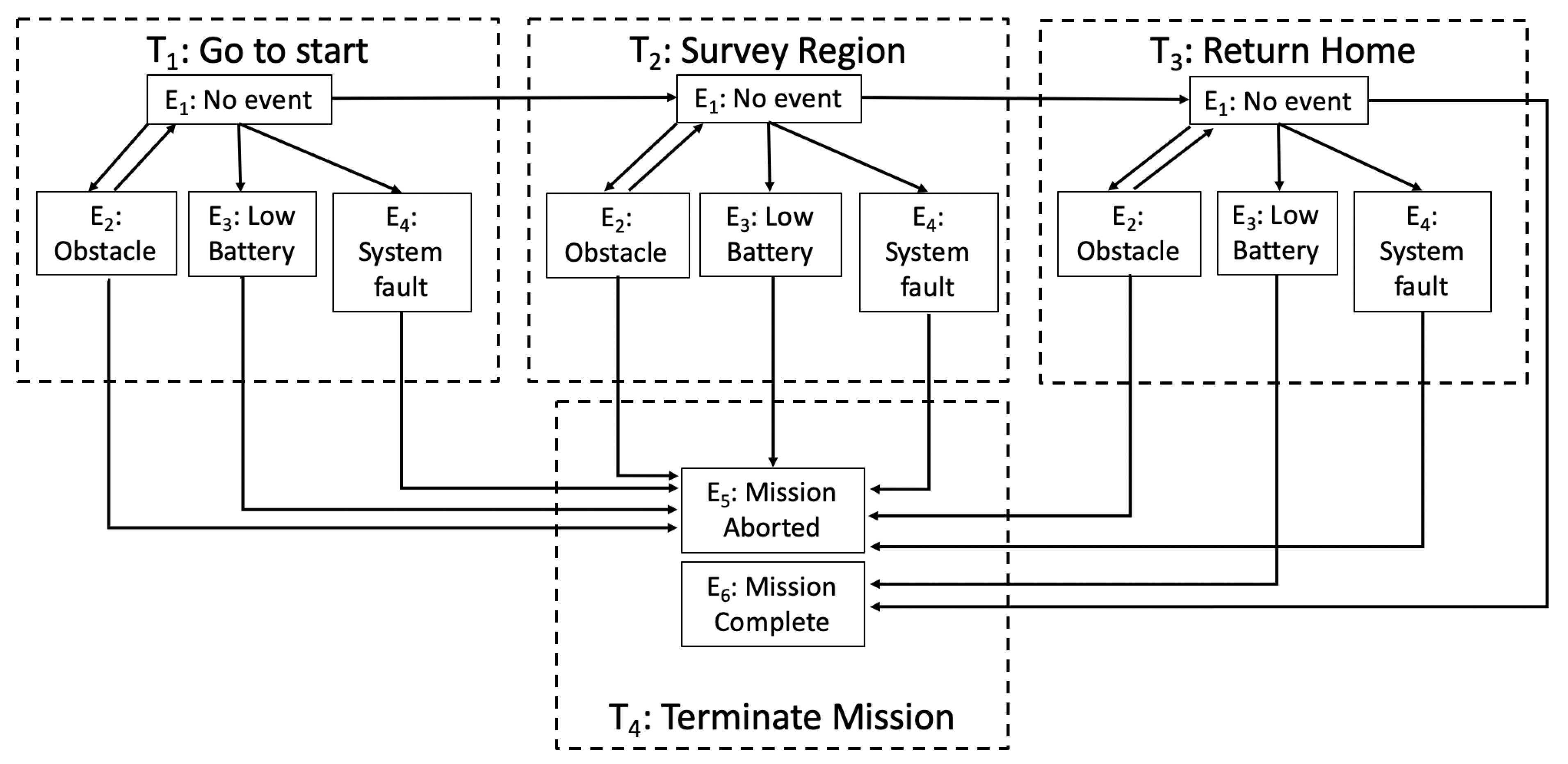
Another useful representation is expressing the mission as a directed graph such that M is defined as the graph, T is the subgraph partitioned by tasks containing a set of vertices, $V_G$, and a set of ordered edges, $E_G$ (Equation (3)). The subscript G differentiates the graph representation from that of the set notation of Equation (2). Mission M may then be represented as:

$$M(T_1(V_G,E_G),T_2(V_G,E_G),...,T_n(V_G,E_G))$$

(3)

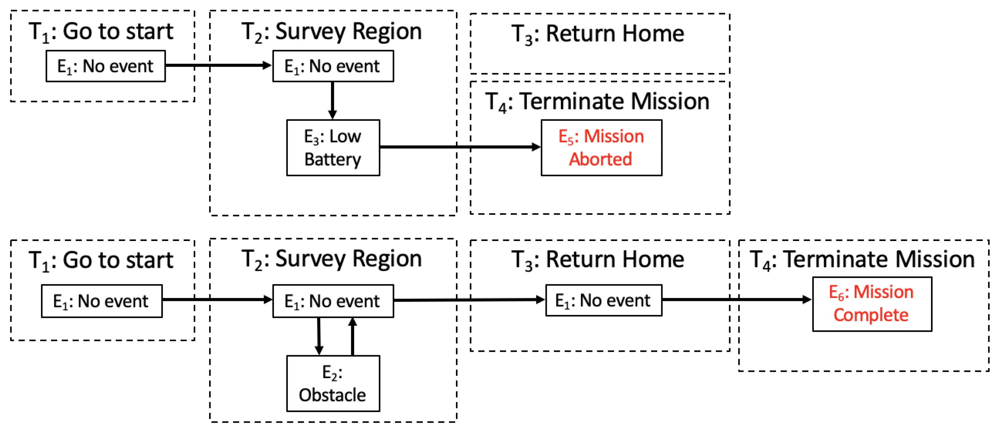
Figure 2 shows an example of this graph structure with the same mission as defined in Figure 1. In Figure 2, insight on relationships between tasks and possible events causing transitions between tasks is observed. Here, the vertices correspond to the possible events and the edges are the possible transitions between events. Behaviors, B, represent the underlying status of the vehicle in response to events and are not shown explicitly in Figure 2 and Equation (3). Figure 3 shows a task and event path for an instance of mission failure versus mission success.

2.2. Fuzzy Logic Overview

Fuzzy Logic (FL) systems and theory, a subset of AI, is employed as the basis for quantifying parameters that describe the performance of a task. An accurate characterization of a system’s performance requires complete knowledge of the mission and the mission requirements, which is often not known a priori [27]. Due to the infinite number of possible scenarios in a given mission and the impracticality of constraining the system and the prevalence of proprietary software, the approach for this research remains independent of internal autonomy architectures [6,8] and defines boundaries on the scope of this work without loss of generality. Additionally, this FL strategy allows flexibility for various definitions of “success” between users (e.g., a defense employee as opposed to a scientist) by weighting performance qualities the user deems important.

Unlike traditional binary logic (i.e., 0, 1), FL utilizes the concept of partial truth (i.e., any value ranging from 0 and 1). This logic more closely resembles how the human brain processes information [24]. In summary, the general FL procedure takes fuzzified input data (via linguistic variables and user-determined membership functions) and processes them through an “if-then” framed rule base, producing a set of fuzzy outputs. These outputs are then combined/weighted into a single output, which is then defuzzified (via another set of membership functions) to produce the final crisp result. First presented by [28], this strategy is often employed in other sectors such as medicine, manufacturing, and business with applications to control systems, decision-making, evaluation, and management. Here, the authors review basic terminology to justify IT2-FL over other forms of FL. FL is the chosen approach for this work due to its ability to provide a strict mathematical framework in which vague and uncertain phenomena can be precisely and rigorously studied [24,27].

2.2.1. Type-1 Fuzzy Logic

In traditional FL theory, a characteristic function allows for various degrees of membership for the elements of a given set. A T1 fuzzy set, A, with a collection of objects X (also referred to as the “universe of discourse”) and elements x, is defined as:

$$A=\left\{(x,{\mu }_A\left(x\right))\right|x\in X\}$$

(4)

where ${\mu }_A$ is the degree of membership of an element x in the set A [27]. These membership functions (MFs) are user selected, often (but not exclusively) incorporating triangular, trapezoidal, and gaussian functions, among others. The MF itself is an arbitrary curve that is chosen for simplicity, convenience, speed, and efficiency. For this application, the fuzzy sets for mission parameters will have defined minimum and maximum thresholds based on the testbed space.

2.2.2. Type-2 Fuzzy Logic

T2-FL was first defined in Zadeh [24], but has gained significant research interest in recent years [22,29]. T2-FL is also referred to as “General T2-FL (GT2-FL)”. A special case of GT2-FL systems is Interval T2-FL (IT2-FL). Both categories of T2-FL are parametric models with additional design degrees-of-freedom to that of a T1-FL system [30,31] and are useful in situations where determining a definitive MF is difficult [22,32].

A T2-FL set is denoted as $\tilde{A}$. As opposed to T1 systems, additional lower (LMF) and upper (UMF) membership functions must also be defined for T2-FL. The corresponding MFs denoted as ${\mu }_{\tilde{A}}^L\left(x\right)$ and ${\mu }_{\tilde{A}}^U\left(x\right)$ for lower and upper bounds, respectively. X now refers to the primary domain, and $J_x$ is now defined as the secondary domain. Rewriting Equation (4) as a General T2 system, $\tilde{A}$ can be defined as (as shown in [29,33]):

$$\tilde{A}=\left\{((x,u),{\mu }_{\tilde{A}}(x,u))\right|\forall x\in X,\forall u\in J_x\subseteq [0,1]\}$$

(5)

What differentiates IT2-FL from GT2-FL is that the IT2-FL uses a uniform secondary MF (i.e., ${\mu }_{\tilde{A}}(x,u)$ = 1), whereas the MF of GT2-FL varies with its secondary membership. As such, the resulting IT2-FL reduces the GT2-FL of Equations (5) to (6) as exemplified in Figure 4, and $\tilde{A}$ reduces to:

$$\tilde{A}=\left\{((x,u),1)\right|\forall x\in X,\forall u\in J_x\subseteq [0,1]\}$$

(6)

Here, since the third dimensional value of the IT2-FL membership is constant, it can be more conveniently represented as a reduced two-dimensional Field of Uncertainty (FOU). For added accuracy and versatility in dealing with MF uncertainties (e.g., vehicle platform uncertainties and sensor noise), the authors choose to implement T2-FL (over T1-FL), and they choose IT2-FL (over GT2-FL) in anticipation of possible data overload burden to maintain computational feasibility, as the GT2-FL approach has been previously shown to introduce design issues and results in high computational costs [31].

As variance quantifies the uncertainty about a variable’s mean in probability theory, the use of IT2-FL enables the quantification of existing uncertainties within a membership function. The FOU is defined as the area bounded by the Lower Membership Function (LMF) and the Upper Membership Function (UMF) and is depicted in the example MF in Figure 5, where the IT2-FL MF is also differentiated from that of a T1-FL. The IT2-FL FOU may be expressed as the union of all primary memberships such that

$$FOU\left(\tilde{A}\right)=\bigcup _{\forall x\in X}({\mu }_{\tilde{A}}^L\left(x\right),{\mu }_{\tilde{A}}^U\left(x\right))$$

(7)

The mapping of the input space to that of the output space is the result of processing the input through a set of “if-then” linguistic rules (e.g., “If x is A, then u is B”). The Fuzzy Inference System (FIS) begins with fuzzifying the crisp input values by using the LMFs and UMFs of the rule antecedent to determine the corresponding degree of membership in terms of linguistic metrics. This step produces two fuzzy values for each IT2-FL MF. Next, the process requires the defuzzification of the fuzzy output set to a crisp output value. The T2 output fuzzy set is reduced (via a “type reducer”) to an Interval T1 fuzzy set resulting in a range, $c_L$ (lower limit) and $c_R$ (upper limit), which is considered the centroid of the T2 fuzzy set. This refers to the average of the centroids of all the type-1 fuzzy sets embedded in the type-2 fuzzy set. The centroid values are calculated iteratively due to the inability to compute exact values for $c_L$ and $c_R$. Methods developed by Karnik and Mendel [34,35] are commonly used with the approximations given as

$$c_L\approx \frac{{\sum }_{i=1}^L{x}_i{\mu }_{\tilde{A}}^U\left(x_i\right)+{\sum }_{i=L+1}^N{x}_i{\mu }_{\tilde{A}}^L\left(x_i\right)}{{\sum }_{i=1}^L{\mu }_{\tilde{A}}^U\left(x_i\right)+{\sum }_{i=L+1}^N{\mu }_{\tilde{A}}^L\left(x_i\right)}$$

$$c_R\approx \frac{{\sum }_{i=1}^R{x}_i{\mu }_{\tilde{A}}^U\left(x_i\right)+{\sum }_{i=R+1}^N{x}_i{\mu }_{\tilde{A}}^L\left(x_i\right)}{{\sum }_{i=1}^R{\mu }_{\tilde{A}}^U\left(x_i\right)+{\sum }_{i=R+1}^N{\mu }_{\tilde{A}}^L\left(x_i\right)}$$

(8)

N denotes the number of samples, $x_i$ is the ith output value sample, and L and R are the left and right estimated switch points, respectively. The defuzzified crisp output value, y, is determined by averaging the two centroid values such that

$$y=\frac{c_L+c_R}{2}$$

(9)

The reader is referred to [35] for further detail on FIS. An overview of the architecture for a T2 Fuzzy systems is provided in Figure 6. Here, the implementation of the Type Reducer differentiates a T2-FL system from that of a T1-FL system.

3. Results

For demonstration purposes (and without loss of generality), PERFORM incorporates two different autonomous path planning techniques for evaluation and direct comparison: (1) a multilayered Potential Field Method/A-Star (PFM/A*) approach [36] and (2) a Probabilistic Roadmap (PRM) method [37]. Details on both algorithms may be found in Appendix A. Both the PFM/A* and PRM techniques are evaluated and compared in the case of three separate mission scenarios:

• Case I: waypoint navigation with single obstacle;
• Case II: waypoint navigation with multiple obstacles;
• Case III: area survey (i.e., lawnmower path survey)

For the given test scenario, an analytical binary occupancy grid is provided to the path planners to differentiate between free and occupied space. It should be noted that the path planners are deliberately left untuned to generate non-optimal paths to better simulate experimental test data and provide higher-integrity data for observing the efficacy of the proof-of-concept IT2-FL autonomy testing and evaluation framework. Routes given are not intended to represent planner capabilities, but to give a reasonable representation of the actual path a vehicle might take given commands generated from the path planners.

For the proposed FL-based evaluation framework and given mission performance criteria, the IT2-FL based autonomy evaluation procedure is summarized as follows:

• Determine user-specified testbed parameters (e.g., the size of the test area and its location, choosing between a two or three-dimensional environment);
• Select the input performance parameters (total distance, time, etc.) of interest;
• Determine appropriate performance measurement tools/criteria (i.e., sensors) and corresponding uncertainty levels (e.g., GPS accuracy limits for measuring navigational coordinates);
• (Optional) use simulations (performed a priori) to provide further context to choosing suitable MF intervals and insight into expected parameter values;
• Generate appropriate MFs using insight gathered from (3) and (4);
• Perform autonomy test missions;
• Gather and post process data from (6) to use as inputs to the IT2-FL Fuzzy Inference System (FIS);
• Obtain overall performance score(s) from IT2-FL evaluation method for final evaluation/comparison of autonomous platform(s)/engine(s).

It is of note that each parameter (performance criteria) may be individually analyzed, in addition to the overall autonomy performance score represented by the final FIS crisp output. The autonomy performance testing method proposed in this paper is intentionally modular and scaleable in design, allowing for testing as simple or complex as the test objectives warrant.

3.1. Test Setup

Laboratory autonomy testing is performed at the Jere A. Chase Ocean Engineering Laboratory (Figure 7a) at the University of New Hampshire (UNH). With dimensions of 18 m × 12 m × 6 m, the UNH Engineering Tank allows for rapid, multi-seasonal testing with both surface and underwater vehicles. The experimental platforms used for this research are small-scale, differential thrust Autonomous Surface Vehicles (ASV), referred to as Testing Unmanned Performance PlatformS (TUPPS). The testbed vehicle has a base width of 0.6 m and a length of 0.9 m and is outfitted with a Velodyne VLP-16 lidar for obstacle detection (Figure 7b). This laboratory test environment is used as the basis for the simulations in this paper to first demonstrate proof-of-concept of PERFORM. It is emphasized that all test data generated for this study are via analytical simulations mimicking test data obtained from the UNH Engineering Tank.

For the first two test cases (Case Study I and Case Study II), the goal of this validation test for PERFORM (from a test engineer’s point-of-view and without loss of generality) is to evaluate a vehicle’s ability to detect an unknown stationary obstacle (if any), replan a path to safely avoid any such obstacles, and to reach the goal waypoint(s) with an acceptable path length. To accomplish this, two performance criteria are selected to evaluate performance: the vehicle’s total distance traveled and the closest point of approach (CPA) to any existing obstacle. These criteria serve as the two inputs to the IT2-FL system. For the third case study (Case III), the goal of the validation test is to evaluate how efficiently the autonomy engine is able to complete an area survey mission, so path percent error and average speed are the chosen inputs. The overall performance score of the path-planning autonomy is the output for all three cases.

3.1.1. PERFORM Case Study I: Single Obstacle

As the first case study, an obstacle configuration given in Figure 8 is simulated to generate experimental test data and analyze the evaluation framework.

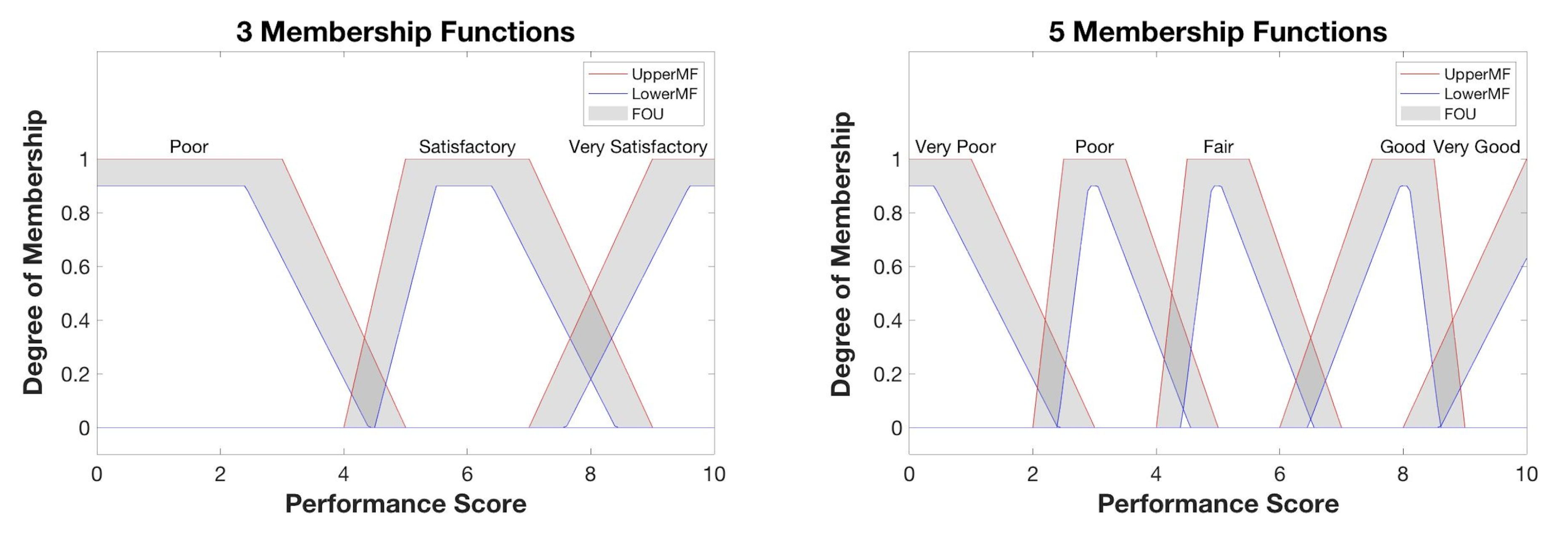
Two different FIS are analyzed (a 3-MF system and 5-MF system) to observe what effects may result (if any) from varying the number of MF’s.

The rule bases for this mission evaluation (arbitrarily chosen and without loss of generality) is summarized in

Table 1. Summary of rules used for a 3-MF system.

Linguistic Term	Close	Adequate	Far
Short	Satisfactory	Very Satisfactory	Satisfactory
Medium	Satisfactory	Very Satisfactory	Satisfactory
Long	Poor	Satisfactory	Poor

and

Table 2. Summary of rules used in the example for a 5-MF system.

Linguistic Term	Very Close	Close	Adequate	Far	Very Far
Very Short	Fair	Good	Very Good	Good	Fair
Short	Fair	Good	Very Good	Good	Fair
Medium	Poor	Fair	Good	Fair	Poor
Long	Very Poor	Poor	Fair	Poor	Very Poor
Very Long	Very Poor	Poor	Fair	Poor	Very Poor

for a 3-MF system and 5-MF system, respectively. Here, the linguistic input terms are italicized with CPA on the horizontal axis and path length given on the vertical axis. The linguistic pattern of Table 1 reads in the following manner:

• If the total distance is short and the CPA is Close, then the performance score is Satisfactory.
• If the total distance is short and the CPA is Adequate, then the performance score is Very Satisfactory.
• …

To encourage the vehicle to remain a safe distance away from an obstacle, the linguistic term “adequate” is mapped to a better performance score. The ideal scenario is to have the vehicle remain a safe distance away from any obstacles while also maintaining the shortest possible path to a given destination within the given test environment.

3.1.2. PERFORM Case Study II: Multiple Obstacles

Similar to Case Study I, the second case study observes a waypoint-to-waypoint task (as shown in Figure 9). In this scenario, two obstacles are present and positioned to analyze the decision-making autonomy of the vehicle with regards to weighting the total distance traveled against vehicle safety (as determined by CPA). To reach the goal, the autonomy engine must decide between maneuvering between the two obstacles and increasing its safety risk or increasing the total distance traveled by taking a more conservative path to avoid the obstacles. Dependent on the intended use of the vehicle, the scoring in the IT2-FL techniques may be modeled to reflect these test goals with appropriate modifications to the rule base. CPA is chosen to be the minimum of the shortest distance between the vehicle and each obstacle. The reader should note that this approach is flexible in its application to an environment with varying numbers of obstacles and types of configurations. For example, an average value calculated from the CPA to each hazard, for instance, may be used instead.

For Case Study II, the rule base (as shown in

Table 3. Summary of rules used for Case Study II.

Linguistic Term	Very Close	Close	Adequate	Far	Very Far
Very Short	Poor	Fair	Good	Very Good	Good
Short	Poor	Fair	Good	Very Good	Good
Medium	Poor	Poor	Fair	Good	Fair
Long	Very Poor	Very Poor	Poor	Fair	Poor
Very Long	Very Poor	Very Poor	Poor	Fair	Poor

) is adjusted to incentivize a heavier weighting of the safety of the vehicle. Here, a higher CPA score corresponds to the linguistic term “far”.

3.1.3. PERFORM Case Study III: Survey Area

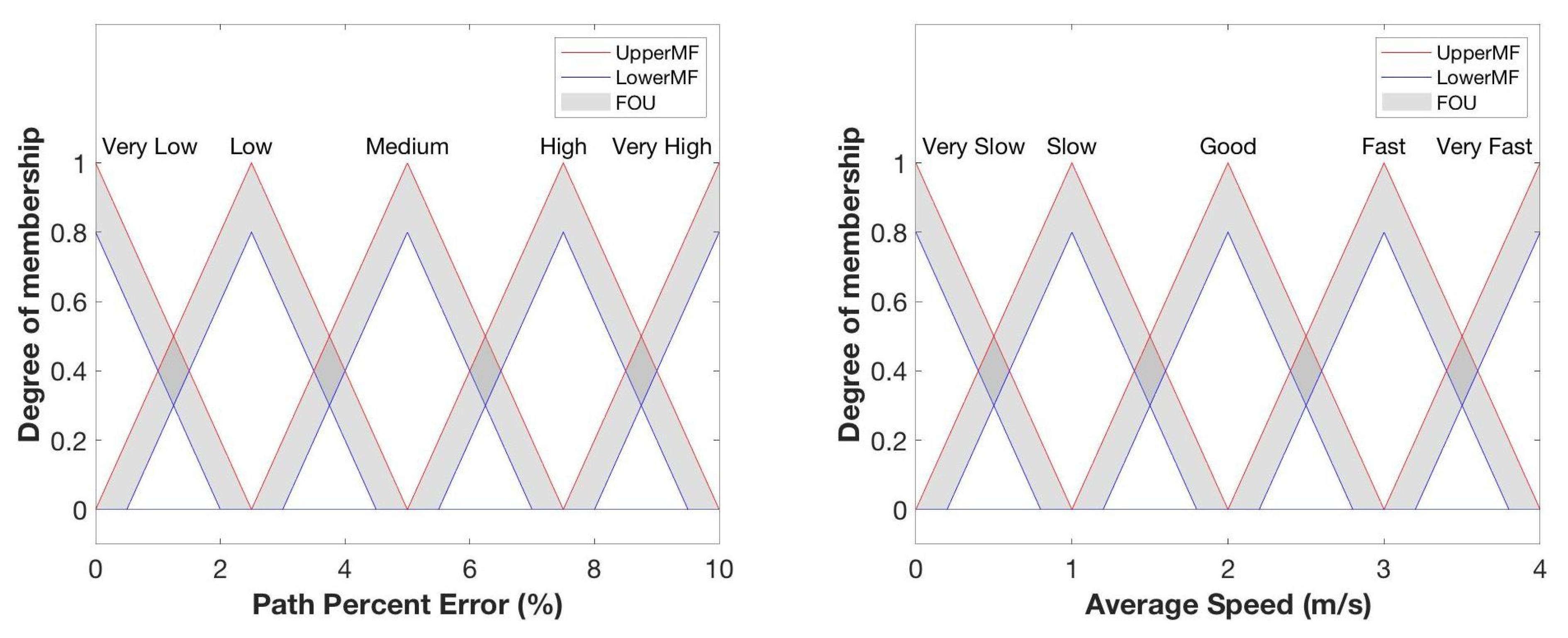
Case Study III analyzes a survey task using a lawnmower pattern (as shown in Figure 10), common for seafloor mapping operations. Different parameters are used to reflect the desired evaluation attributes. Due to mapping operations relying on swath widths based on depth to minimize gaps in coverage, path percent error, the percent error between the actual route the vehicle takes compared to the desired lawnmower pattern, is one of the parameters measured. The second parameter is average vehicle speed. A consistent vehicle speed within the optimal range of the sonar is also important for high quality data.

The rule base for Case III is constructed to reflect a narrower region for acceptable performance and shown in

Table 4. Summary of rules used for Case Study III.

Linguistic Term	Very Slow	Slow	Good	Fast	Very Fast
Very Low	Poor	Fair	Very Good	Fair	Poor
Low	Poor	Fair	Very Good	Fair	Poor
Medium	Poor	Poor	Fair	Poor	Poor
High	Very Poor	Very Poor	Very Poor	Very Poor	Very Poor
Very High	Very Poor	Very Poor	Very Poor	Very Poor	Very Poor

. To receive a higher performance score, the vehicle’s average speed should remain in the “good” range window while maintaining low error over the path taken.

3.2. Membership Function Construction

3.2.1. PERFORM Input Parameters

There are various ways to generate MFs to best suit the intentions of the autonomy test engineer. For this application, each testbed sensor used for PERFORM includes fuzzy MFs to account for specific sensor characteristics and uncertainties. For example, total distance traveled is determined using GPS. The uncertainty in the GPS measurement, found experimentally or those provided by product specifications/documentation, is integrated into the MF FOU. Sensor measurement quality can also be affected by sources such as high noise levels and changing environmental conditions (e.g., humidity, rain, etc.) [35,38]. If desired, these methods may also benefit from added knowledge from a priori simulations giving further context to suitable measurement ranges/bandwidths and corresponding MF intervals for a given testbed.

It is assumed that the sensors and vehicle are identical to enable the direct comparison of the path planning algorithms. The positioning system used for this testbed is a Marvelmind HW v4.9-NIA indoor positioning system. By taking into account the measurement noise produced from this signal, improvements are expected for the IT2-FL techniques [20]. Marvelmind company documentation gives a measurement uncertainty value of ±0.02 m [39]. From the obstacle configuration given in Figure 8, the shortest path to the goal location (including the obstacle) based on Euclidean distance is used as the minimum of the input range for total distance. The maximum distance used in the MF is arbitrarily defined to be twice the minimum distance and can be adjusted depending on the user’s acceptable tolerance. Any test run value greater than the maximum will automatically be input at this saturated maximum value.

The “total distance” in this work is calculated by determining the overall sum of the changes in position such that

$$\sum _{k=1}^n{d}_k=\sqrt{{(x_k-x_{k-1})}^2+{(y_k-y_{k-1})}^2}$$

(10)

where k, n, and d represent the measurement number, total number of measurements, and corresponding distance, respectively. To determine an appropriate uncertainty value, the authors choose to calculate the combined uncertainty, $u_c$, using a $l^2-$ norm such that

$$u_c=\sqrt{u^2\left(x_1\right)+u^2\left(x_2\right)+u^2\left(x_3\right)+...+u^2\left(x_n\right)}$$

(11)

where $\mu \left(x_i\right)$ represents the uncertainty at position measurement $x_i$.

The number of measurements for a given test run is dependent on two factors: the sampling rate and total test time. It is assumed here that the sampling rate for the vehicle’s position is the same for each specific mission or task. A value of ±0.75 m is determined as a reasonable value for this case study based on previously observed test platform speeds and time ranges (results not shown here). Since determining the vehicle’s CPA to the obstacle relies on a singular measurement, the uncertainty value of ±0.02 m from the company’s documentation is used as the FOU width for CPA related MFs.

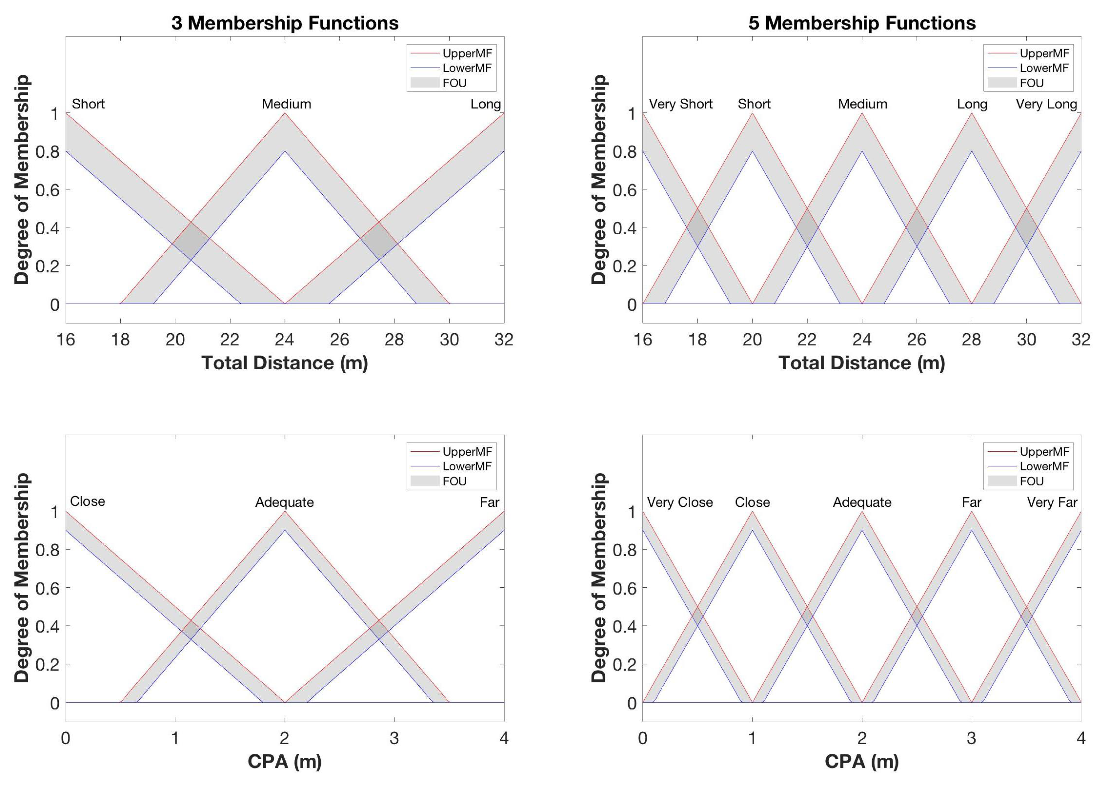
A summary of the evaluation parameter ranges and uncertainties for both total distance and CPA are provided in

Table 5. Range of values for construction of Case Study I and II MFs.

Evaluation Parameter	Total Distance (m)	CPA (m)
Range	16.00–32.00	0–4.00
Uncertainty	±0.75	±0.02

. From these values, the input MF’s for total distance and CPA are given in Figure 11. The same input MF’s are used for Case Study I and II (with II using only the 5-MF system).

For Case Study III, the MFs are modified to represent the new parameters (path percent error and average speed) under this test environment and is shown in Figure 12. Both parameters use data from the testbed GPS unit, so the uncertainty bounds are designed to take this into account. Path percent error and average speed are 0.50% and 0.25 m/s, respectively, and are deemed appropriate for the level of accuracy warranted in this case study. Variable ranges for Case III are summarized in

Table 6. Range of values for construction of Case Study III MFs.

Evaluation Parameter	Path Percent Error	Average Speed (m/s)
Range	0–10	0–4.0
Uncertainty	+/− 0.50	+/− 0.25

.

3.2.2. PERFORM Output

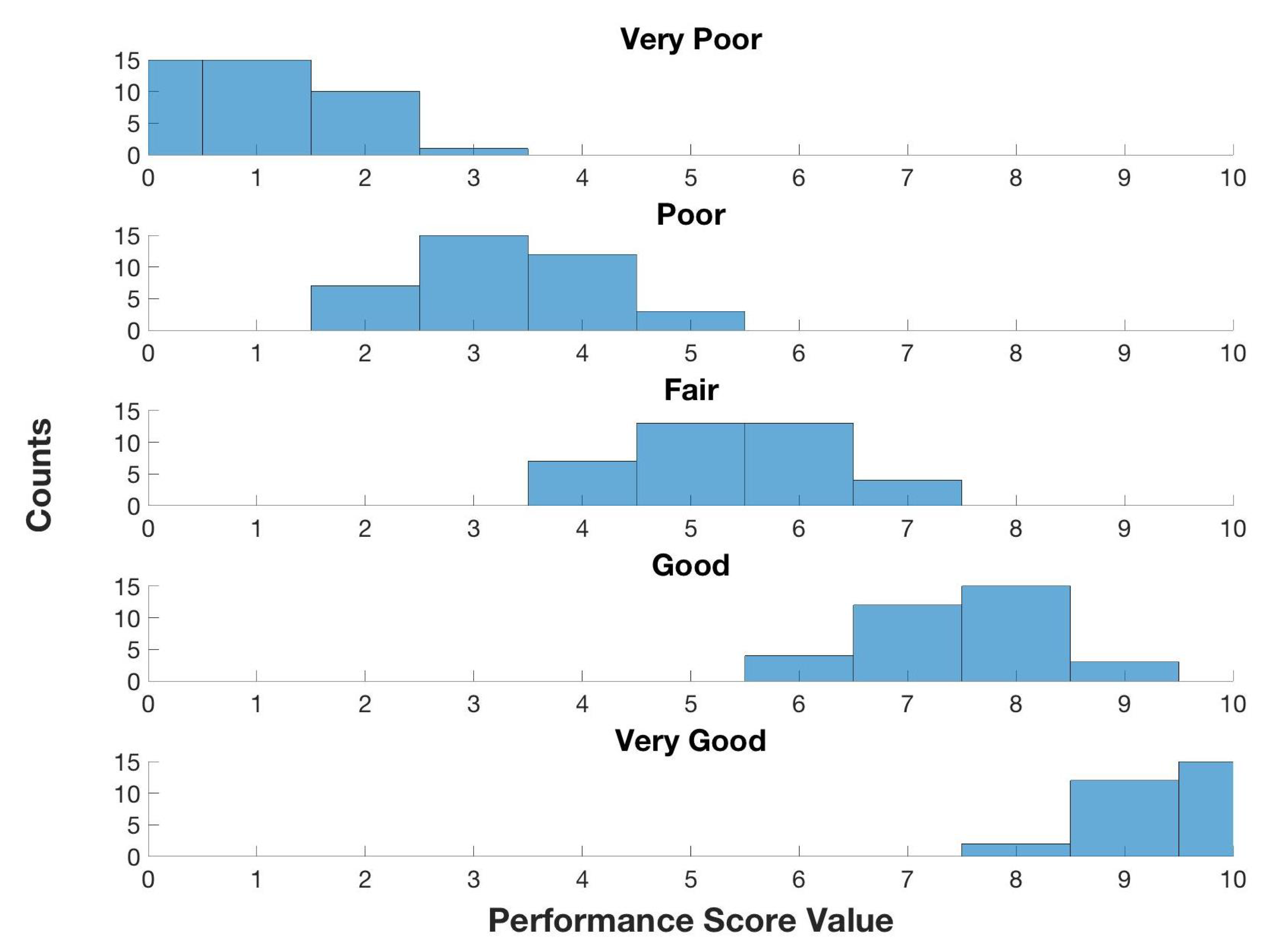
For the construction of the performance score MFs, a different approach is used to show the variety of factors that may be incorporated. The same performance MFs are used for Case Studies I, II, and III. The uncertainty in these MF’s originate from the uncertainty in the linguistic terms. Linguistic terms tend to be subjective, or rather that these terms have different meanings to different individuals and thereby create yet another level of vagueness [35]. To address this, a separate study was performed where several individuals (members of the University of New Hampshire marine robotics teams) were polled to provide their opinions regarding the relations of linguistic terms to numerical values in order to construct the MFs. The resulting MFs are shown in Figure 13. Poll data and corresponding histograms are given in the Appendix B (Figure A1 and Figure A2).

3.3. PERFORM Test Results

3.3.1. Case Study I: PERFORM Results

The MF relationships between the input and output variables can be visualized as a 3D plot (Figure 14). This view shows the ideal parameters value, designated in yellow on the color scale and displayed as the maximum value on the z-axis. The objective for the vehicle in this case study, reflected in the rule base and defined numerically in the MFs, is to maintain a safe distance, determined as 2 m, while minimizing the total distance to the goal (i.e., desired waypoint). As shown, the yellow portion of the plot corresponds to these goals spanning the area defined by a 2 m CPA and the region extending from 0 m to roughly 24 m of total distance traveled.

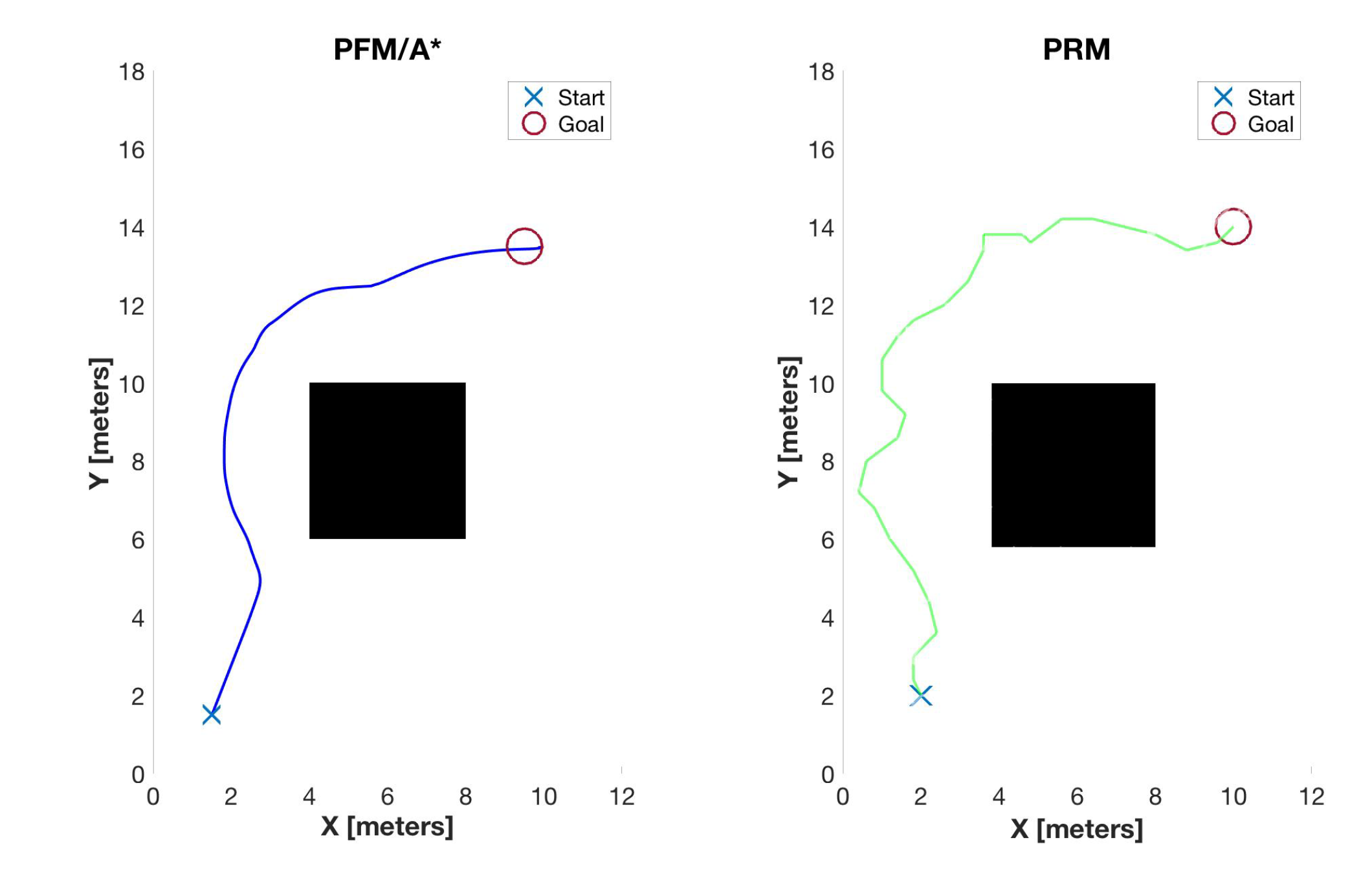
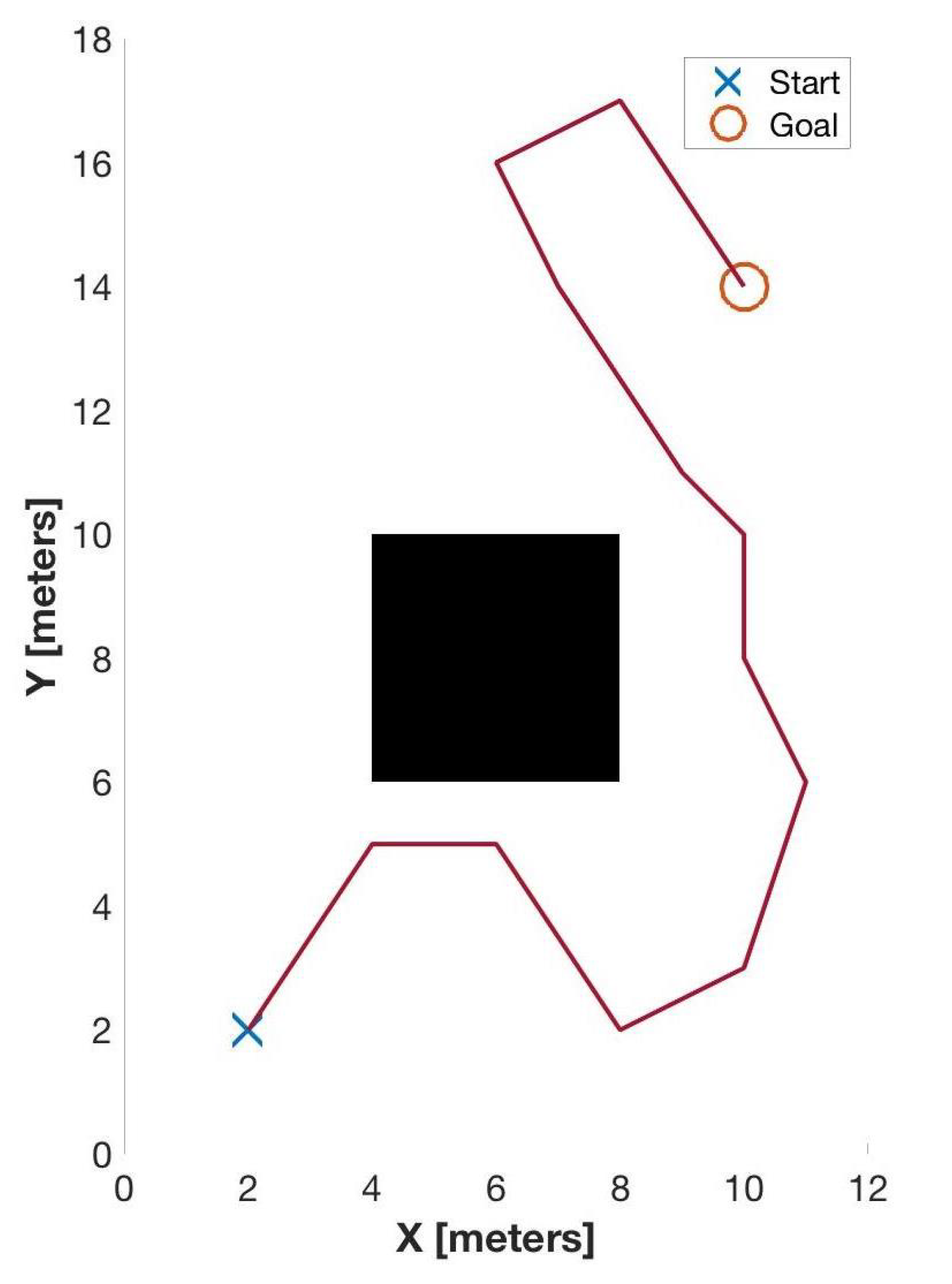
Figure 15 provides a side-by-side comparison between the PFM/A* path planning method (left) and that of the PRM method (right).

Table 7. Summary of simulated performance values for Case Study I.

Evaluation Parameter	Total Distance (m)	CPA (m)
PFM/A*	19.28	1.50
PRM	21.52	2.48
Generic Path	31.92	1.00

summarizes the simulated performance parameter values. An additional route is given in Figure 16 for additional context to demonstrate a path that would generate a poor score. This route (referred to as a “Generic Planner”) is significantly more circuitous than either of the PFM/A* and PRM methods and also traverses much closer to the obstacle than is desired.

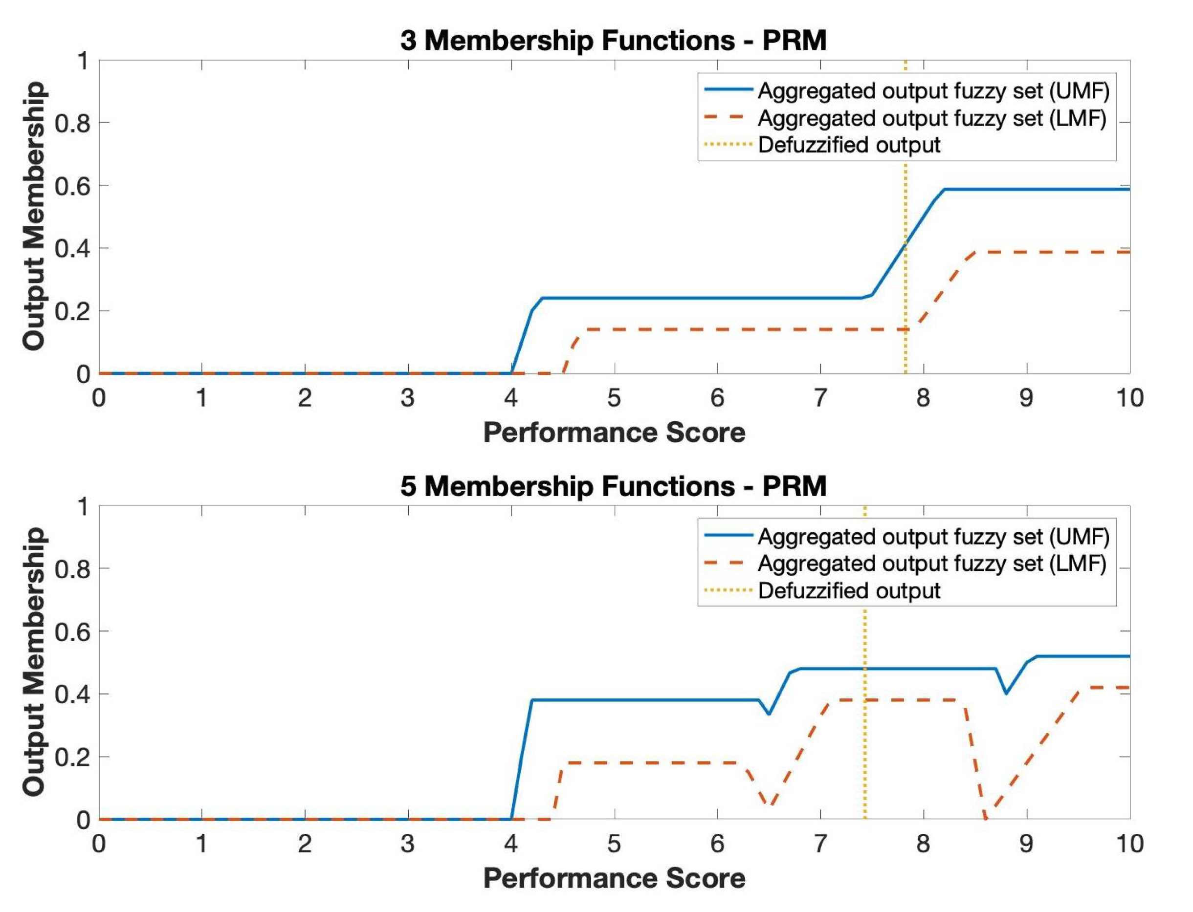
Performance score results from applying the FIS to the input values in Table 7 are shown in

Table 8. Performance Score Output for Case Study I.

Path Planning Algorithm	3 Membership Functions	5 Membership Functions
PFM/A*	7.79	8.24
PRM	7.82	7.43
Generic Planner	3.67	3.30

. The resulting output fuzzy set overlaid by the defuzzified outputs given in Table 8 are shown in Figure 17 and Figure 18 for both 3-MF and 5-MF based systems for the PRM and PFM/A* planners, respectively. Visual observation shows that the PFM/A* route has the best performance given the mission goals. As expected, the generic planner scores the lowest. The difference in scores between the PRM and PFM/A* autonomy methods are negligible in the 3-MF case (0.03) and more obvious in the 5-MF case (0.81).

3.3.2. Case Study II: PERFORM Results

The 5-MF colormap for Case Study II is provided in Figure 19. In accordance with the test goals for this case study, the MFs incentivize the more conservative CPA scores (roughly 3 m distance) while again minimizing the total distance covered by the vehicle. The highest performance score values are designated in yellow. The resulting simulated paths are shown in Figure 20. The corresponding table,

Table 9. Summary of simulated performance values for Case Study II.

Evaluation Parameter	Total Distance (m)	CPA (m)
PFM/A*	21.16	1.47
PRM	16.90	0.81

, presents the parameters values from the test run.

After applying the rule base and MF’s using the test run values given in Table 9, the evaluation results are given in

Table 10. Performance Score Output for Case Study II.

Path Planning Algorithm	Performance Score
PFM/A*	5.90
PRM	4.96

. The output fuzzy set with the defuzzified value is shown in Figure 21. While both planners succeed at avoiding the obstacle and arriving at the desired waypoint, the more conservative route taken by the PFM/A* vehicle (although corresponding to a longer distance traveled than that of the PRM vehicle) is given the better score, which is consistent with the modeled rule base MFs and mission objectives.

3.3.3. Case Study III: PERFORM Results

The resulting MF 3D plot for Case Study III depicts the correlations between the evaluation parameters and the performance score (Figure 22). Noted in the colormap is the smaller, more distinct area corresponding with the best performance scores (in yellow) meant to model stricter standards for performance. With the simulated path outputs given in Figure 23 and the resulting parameters values (

Table 11. Summary of simulated performance values for Case Study III.

Evaluation Parameter	Path Percent Error	Average Speed (m/s)
PFM/A*	1.43	1.50
PRM	6.71	2.50

), the final scores are presented in

Table 12. Performance Score Output for Case Study III.

Path Planning Algorithm	Performance Score
PFM/A*	6.94
PRM	2.78

and the full output fuzzy set is given in Figure 24. Both routes successfully complete the given seafloor mapping mission. However, it is clear (as seen in Figure 24 and numerically indicated in Table 11) that the PFM/A* vehicle takes a smoother and more direct path, resulting in a lower path percent error.

4. Discussion

This study presented the Performance Evaluation and Review Framework of Robotic Missions (PERFORM), a flexible but rigorous method to validate autonomous vehicles in testbed environments using a unique IT2-FL performance evaluation framework. The use of FL allows for test parameters that are tailored to the user’s design requirements and can account for different priorities related to acceptable risks and goals of a given mission. The 3D renderings presented show parameter values for a specific mission across the space of reasonable test results in relation to a performance score output. This, in addition to the decomposition of a mission, M, into tasks, T (Equation (2)), reduces the number of test runs necessary with the ability to analyze different scenarios taking on a range of values. Translating into both a time and cost savings, this may limit the need to perform a large number of sets of simulations, which can have difficulty modeling the ocean environment accurately, testing sensor perception capabilities, and predicting other hardware issues. Results indicate that these methods aid in direct comparison of path planning algorithms as presented in the case studies with broader applications to other high-level validation test objectives such as autonomous behavior analysis.

In viewing the results for Case Study I, the 3-MF system resulted in a negligible difference in scores. The 5-MF system, however, allowed for an easier differentiation of scores due to increased value sensitivity, producing a more substantial difference in value. One should weigh the number of included MFs based on a balance of available test design time and desired score resolution. A quick and simple study could utilize a 3-MF system, while a higher MF system (in this case, a 5-MF system) can be designed if increased complexity is needed.

In Case Study II, analyzing behavior regarding balancing risk with efficiency, the PFM/A* path taken to avoid the obstacles received a better score than that of the PRM path. This was predicted as the FIS was intentionally modeled to incentivize conservative decisions by the vehicle in the final performance score. During general implementation, there may be test cases where evaluation parameters will appear to have conflicting goals such as in this scenario—safety vs. efficiency. The user, then, must determine the acceptable risk and hierarchy of performance priorities and reflect this in the modeling of the system.

The final scenario, Case Study III, took a stricter approach to a vehicle, receiving a desirable score. As shown in Figure 22, there is a steeper decline to poorer performance values. In some applications, there is a strict cutoff of acceptable performance. The National Oceanic and Atmospheric Administration (NOAA), for instance, has set hydrographic surveying standards that are required to be met for data to be utilized by the organization [40]. With this in mind, the evaluation model has the ability to incorporate these standards in the design of both the MF’s and the rule base.

PERFORM becomes streamlined once a testbed environment is established and common measurement sensors are incorporated and calibrated. Many testing scenarios can be evaluated with the incorporation of minor changes, which would depend on given specific testing goals. The authors envision a library (expanded upon over time) of testing parameters with the x-axis MF range being the only necessary change based on the specific task under test. Once the MFs are created and the test foundation is constructed by a test engineer, the linguistic aspect of FL may be more approachable for various parties to understand and to set vehicle autonomy expectations in order to show “success.” The linguistic base encourages a common language between engineers, operators, researchers, and program managers that all disciplines understand.

In perspective of other studies in the area of autonomous system test and evaluation, PERFORM may be useful as an extension of the JHU simulations [6] (referred to in Section 1) to find boundary cases. These boundary cases are a subset of all possible scenarios, and could provide a feasible number of cases to undergo experimental testing.

Future work will apply PERFORM to the TUPPs experimental platform for acquiring experimental field test data while also testing different mission types and scenarios. Further analysis of different MF shapes, FOU sizes, and additional input variables on the output will undergo investigation as well as constructing methods for accommodating the design of MFs for time-series based data input.

5. Conclusions

With a goal of establishing a preliminary foundation for designing and evaluating autonomy tests for autonomous vehicles, this paper introduces the Performance Evaluation and Review Framework of Robotic Missions (PERFORM). PERFORM demonstrates the feasibility of applying fuzzy logic, namely an IT2-FL strategy, as an effective and efficient evaluation framework for assessing autonomous vehicles in a scalable testbed environment with the ability to further generalize the methods for different mission types and scenarios. The proposed method decomposes a mission with respect to event and behavior-based tasks. Through three case studies, results support these claims and contribute a unique approach towards testing autonomy that is independent of internal autonomy architectures. By designing MF’s and FOU bounds, uncertainties due to sensor noise, environmental conditions, and the inherent vagueness of linguistic terms may be added. Overall, PERFORM is mathematically rigorous, yet flexible for the user’s intended test goals. The proposed framework and methodologies presented in this work represent the first crucial step in developing a standard for comparing and evaluating autonomy performance.

References

Bouchard, A.; Tatum, R. Verification of Autonomous Systems: Challenges of the Present and Areas for Exploration. In Proceedings of the OCEANS 2015—MTS/IEEE, Washington, DC, USA, 19–22 October 2015; pp. 1–10. [Google Scholar]
Dutta, R.; Guo, X.; Jin, Y. Quantifying Trust in Autonomous System Under Uncertainties. In Proceedings of the 29th IEEE International System-on-Chip Conference (SOCC), Seattle, WA, USA, 6–9 September 2016; pp. 362–367. [Google Scholar]
Liu, Z.; Zhang, Y.; Yu, X.; Yuan, C. Unmanned surface vehicles: An overview of developments and challenges. Annu. Rev. Control.2016, 41, 71–93. [Google Scholar] [CrossRef]
Song, R.; Liu, Y.; Bucknall, R. A multi-layered fast marching method for unmanned surface vehicle path planning in a time-variant maritime environment. Ocean. Eng.2017, 129, 301–317. [Google Scholar] [CrossRef]
Grotli, E.; Reinen, T.; Grythe, K.; Transeth, A.; Vagia, M.; Bjerkeng, M.; Rundtop, P.; Svendsen, E.; Rodseth, O.; Eidnes, G. Seatonomy. In Proceedings of the OCEANS 2015—MTS/IEEE, Washington, DC, USA, 19–22 October 2015; pp. 1–7. [Google Scholar]
Mullins, G.; Stankiewicz, P.; Hawthorne, R.; Appler, J.; Biggins, M.; Chiou, K.; Huntley, M.; Stewart, J.; Watkins, A. Delivering test and evaluation tools for autonomous unmanned vehicles to the fleet. Johns Hopkins APL Tech. Dig.2017, 33, 279–288. [Google Scholar]
Redfield, S.; Seto, M. Verification challenges for autonomous systems. In Autonomy and Artificial Intelligence: A Threat or Savior? Lawless, W., Mittu, R., Sofge, D., Russell, S. Eds.; Springer International Publishing: Berlin/Heidelberg, Germany, 2017; pp. 103–127. [Google Scholar]
Betts, K.; Petty, M. Automated search-based robustness testing for autonomous vehicle software. Model. Simul. Eng.2016, 2016, 5309348. [Google Scholar] [CrossRef]
Mullins, G.; Stankiewicz, P.; Gupta, S. Automated generation of diverse and challenging scenarios for test and evaluation of autonomous vehicles. In Proceedings of the 2017 IEEE International Conference on Robotics and Automation (ICRA), Singapore, 29 May–3 June 2017; pp. 1443–1450. [Google Scholar]
Durst, P.; Gray, W. Levels of Autonomy and Autonomous System Performance Assessment for Intelligent Unmanned Systems. US Army Corps of Engineers, Engineer Research and Development Center, Geotechnical and Structures Laboratory. Available online: https://apps.dtic.mil/dtic/tr/fulltext/u2/a601656.pdf (accessed on 13 May 2020).
Hrabia, C.; Masuch, N.; Albayrak, S. A Metrics Framework for Quantifying Autonomy in Complex Systems. In Multiagent System Technologies; Müller, J., Ketter, W., Kaminka, G., Wagner, G., Bulling, N., Eds.; Springer International Publishing: Berlin/Heidelberg, Germany, 2015; pp. 22–41. [Google Scholar]
Olszewska, J.; Barreto, M.; Bermejo-Alonso, J.; Carbonera, J.; Chibani, A.; Fiorini, S.; Goncalves, P.; Habib, M.; Khamis, A.; Olivares, A.; et al. Ontology for Autonomous Robotics. In Proceedings of the 26th IEEE International Symposium on Robot and Human Interactive Communication (RO-MAN), Lisbon, Portugal, 28 August–1 September 2017; pp. 189–194. [Google Scholar]
Menzel, T.; Bagschik, G.; Maurer, M. Scenarios for Development, Test and Validation of Automated Vehicles. In Proceedings of the 2018 IEEE Intelligent Vehicles Symposium (IV), Changshu, China, 26–30 June 2018; pp. 1821–1827. [Google Scholar]
Kalra, N.; Paddock, S. Driving to Safety: How Many Miles of Driving Would It Take to Demonstrate Autonomous Vehicle Reliability? RAND Corporation: Santa Monica, CA, USA, 2016; Available online: https://www.rand.org/pubs/research_reports/RR1478.html (accessed on 11 May 2020).
Huang, H. Autonomy levels for unmanned systems (ALFUS) framework: Safety and application issues. In Proceedings of the 2007 Workshop on Performance Metrics for Intelligent Systems, Baltimore, MA, USA, 28–30 August 2007; pp. 48–53. [Google Scholar]
Durst, P.; Gray, W.; Nikitenko, A.; Caetano, J.; Trentini, M.; King, R. A framework for predicting the mission-specific performance of autonomous unmanned systems. In Proceedings of the 2014 IEEE/RSJ International Conference on Intelligent Robots and Systems, Chicago, IL, USA, 14–18 September 2014; pp. 1962–1969. [Google Scholar]
Sun, Y.; Xiong, G.; Song, W.; Gong, J.; Chen, H. Test and Evaluation of Autonomous Ground Vehicles. Adv. Mech. Eng.2014, 6, 1–13. [Google Scholar] [CrossRef]
Xiong, G.; Zhao, X.; Liu, H.; Wu, S.; Gong, J.; Zhang, H.; Tan, H.; Chen, H. Research on the Quantitative Evaluation System for Unmanned Ground Vehicles. In Proceedings of the 2010 IEEE Intelligent Vehicles Symposium, San Diego, CA, USA, 21–24 June 2010; pp. 523–527. [Google Scholar]
Mendel, J. Type-2 Fuzzy Sets: Some Questions and Answers. IEEE Connect. Newsl. IEEE Neural Netw. Soc.2003, 1, 10–13. [Google Scholar]
Linda, O.; Manic, M. Uncertainty Modeling for Interval Type-2 Fuzzy Logic Systems Based on Sensor Characteristics. In Proceedings of the 2011 IEEE Symposium on Advances in Type-2 Fuzzy Logic Systems (T2FUZZ), Paris, France, 11–15 April 2011; pp. 31–37. [Google Scholar]
Wu, D.; Mendel, J. Uncertainty Measures for Interval Type-2 Fuzzy Sets. Inf. Sci.2007, 177, 5378–5393. [Google Scholar] [CrossRef]
Garibaldi, J.; Musikasuwan, S.; Ozen, T. The Association between Non-Stationary and Interval Type-2 Fuzzy Sets: A Case Study. In Proceedings of the 14th IEEE International Conference on Fuzzy Systems, Reno, NV, USA, 25–27 May 2005; pp. 224–229. [Google Scholar]
Zadeh, L. The concept of a linguistic variable and its application to approximate reasoning. Inf. Sci.1975, 8, 199–249. [Google Scholar] [CrossRef]
Roberts, W.; Meyer, P.; Seifert, S.; Evans, E.; Steffens, M.; Mavris, D. A Flexible Problem Definition for Event-Based Missions for Evaluation of Autonomous System Behavior. In Proceedings of the OCEANS 2018 MTS/IEEE, Charleston, SC, USA, 22–25 October 2018; pp. 1–7. [Google Scholar]
Zimmermann, H. Fuzzy Set Theory and Its Applications, 4th ed.; Springer: New York, NY, USA, 2001. [Google Scholar]
Castillo, O.; Amador-Angulo, L.; Castro, J.; Garcia-Valdez, M. A comparative study of type-1 fuzzy logic systems, interval type-2 fuzzy logic systems and generalized type-2 fuzzy logic systems in control problems. Inf. Sci.2016, 354, 257–274. [Google Scholar] [CrossRef]
Castillo, O.; Aguilar, L. Type-2 Fuzzy Logic in Control of Nonsmooth Systems: Theoretical Concepts and Applications; Springer International Publishing: Berlin/Heidelberg, Germany, 2019. [Google Scholar]
Mendel, J. General Type-2 Fuzzy Logic Systems Made Simple: A Tutorial. IEEE Trans. Fuzzy Syst.2014, 22, 1162–1182. [Google Scholar] [CrossRef]
Mendel, J. Type-2 Fuzzy Sets and Systems: An Overview. IEEE Comput. Intell. Mag.2007, 2, 20–29. [Google Scholar] [CrossRef]
Sola, H.; Fernandez, J.; Hagras, H.; Francisco, H.; Pagola, M.; Barrenechea, E. Interval Type-2 Fuzzy Sets are Generalization of Interval-Valued Fuzzy Sets: Toward a Wider View on Their Relationship. IEEE Trans. Fuzzy Syst.2015, 23, 1876–1882. [Google Scholar] [CrossRef]
Karnik, N.; Mendel, J. Centroid of a type-2 fuzzy set. Inf. Sci.2001, 132, 195–220. [Google Scholar] [CrossRef]
Mendel, J.; Hagras, H.; Tan, W.; Melek, W.; Ying, H. Introduction to Type-2 Fuzzy Logic Control; IEEE Press: Hoboken, NJ, USA, 2014. [Google Scholar]
Dalpe, A.; Cook, A.; Thein, M.-W.; Renken, M. A Multi-Layered Approach to Autonomous Surface Vehicle Map-Based Autonomy. In Proceedings of the OCEANS 2018 MTS/IEEE, Charleston, SC, USA, 22–25 October 2018; pp. 1–8. [Google Scholar]
Kavraki, L.; Svestka, P.; Latombe, J.; Overmars, M. Probabilistic roadmaps for path planning in high-dimensional configuration spaces. IEEE Trans. Robot. Autom.1996, 12, 566–580. [Google Scholar] [CrossRef]
Benatar, N.; Aickelin, U.; Garibaldi, J. Performance Measurement Under Increasing Environmental Uncertainty in the Context of Interval Type-2 Fuzzy Logic Based Robotic Sailing. arXiv2013, arXiv:1308.5133. [Google Scholar] [CrossRef]
Figure 1.
Example seafloor mapping mission with associated tasks and behaviors.
Figure 2.
Graphical overview of the example mission for a given scenario.
Figure 3.
Example of a task and event flow for mission failure (top) vs. mission success (bottom).
Figure 4.
Example of a GT2-FL (left) vs. IT2-FL (right) Fuzzy Set.
Figure 5.
Example membership functions for T1 (left) and T2 (right) Fuzzy Systems.
Figure 6.
T2-FL System.
Figure 7.
(a) The Chase Engineering Tank located at the University of New Hampshire (b) Small-Scale ASV Experimental Platform. Simulations are based upon the laboratory equipment shown here.
Figure 8.
Testbed for Case I (obstacle represented by the black box).
Figure 9.
Testbed for Case Study II (obstacles represented by black boxes).
Figure 10.
Testbed setup for Case Study III: A lawnmower pattern to perform seafloor mapping operations.
Figure 11.
Membership functions for total distance and CPA.
Figure 12.
Membership functions for Case Study III to observe path percent error and average vehicle speed.
Figure 13.
Membership functions for the performance score output.
Figure 14.
3D plot MFs relating input variables (total distance and CPA) with corresponding output variables (performance scores).
Figure 16.
Generic Planner: An example of a poorly traveled path.
Figure 17.
Output set for the PFM/A* algorithm.
Figure 18.
Output set for the PRM algorithm.
Figure 19.
Case Study II 5-MF 3D plot relating the input variables (total distance and CPA) with corresponding output variables (performance scores).
Figure 20.
Case Study II: PFM/A* generated path (left), PRM generated path (right).
Figure 21.
Output set for Case Study II.
Figure 22.
Case Study III 5-MF 3D plot relating the input variables (path percent error and average vehicle speed) with the corresponding performance scores.
Figure 23.
Case Study III simulated path output.
Figure 24.
Output set for Case Study III.