The Spatial Structure of Passively Simulated Atmospheric Boundary Layer Turbulence

Featured Application

This study conducted an investigation on the spatial structure of large-scale boundary layer turbulence simulated by a wind tunnel, and through comparative analysis with isotropic turbulence theory, some improved coherence models are proposed based on the experimental results.

Abstract

Three types of turbulence fields were investigated using a research method combining wind tunnel tests and theoretical analysis to further explore the spatial structure of atmospheric boundary layer turbulence, which was passively simulated by a wind tunnel. The fundamental theory of turbulence is introduced, and some traditional theoretical coherence models based on isotropic turbulence theory are derived. The difference between the theoretical results and the passive simulation of atmospheric boundary layer turbulence was compared and discussed. The analysis results show that the passively simulated atmospheric turbulence basically conformed to the homogeneous isotropic turbulence assumption on the horizontal plane, but the interference of the nonisotropic turbulence components cannot be ignored either. Finally, some improvements were made to the traditional coherence function model based on the experimental results to apply the passively simulated atmospheric boundary layer turbulence.

1. Introduction

The spatial structure of atmospheric boundary layer turbulence is one of the most critical studies in turbulence theory and is also a core subject in a variety of fields, such as transportation, aircraft, and structural wind engineering [1]. Some turbulence parameters such as the average wind speed, integral length scale, fluctuating wind spectrum, and coherence function are the fundamental functions of wind load prediction and wind-induced vibration evaluation of structures, particularly in the design of wind-sensitive structures [2]. Meanwhile, the study of the spatial structure of atmospheric boundary layer turbulence is extremely difficult. There are still many problems that have not yet been fully understood due to its many influencing factors [3,4]. It is necessary to conduct extensive research.

According to the current research progress, the main research methods include natural wind field measurements, wind tunnel tests, numerical simulations, and theoretical research. Field measurement is the most direct and effective method to obtain the 3D characteristics of boundary layer turbulence. Kaimal et al. [5], Solari [6], Kareem [7], Mann [8], and Simiu et al. [9] previously used the field measurements from monsoons or typhoons to study turbulence characteristics and proposed classic turbulence models that are still widely used today. Statistical analyses on the main characteristic parameters of boundary layer turbulence, including the wind profile, integral scale, wind spectrum, and coherence function, were conducted by Li [10], Cao [11], Fenerci [12], Tao [13], and Zhao [14], among others, and they provided valuable references for engineering practice. Although field measurement plays an important role in the study of turbulence characteristics, it must be noted that it is generally difficult to achieve due to uncontrollable factors such as the long measurement period and high costs [15].

Many researchers have studied the spatial characteristics of the boundary layer using theoretical analyses or numerical simulations, resulting in a variety of solutions to complex turbulence problems [1,3,8,16,17]. Many classic turbulence theory models, such as isotropic turbulence theory and related improved models, have been developed [1,3,5,18]. However, deriving the turbulence theory and solving the motion equation are extremely difficult [2,9,19]. Although turbulent problems can be solved using a variety of assumptions and simplifications, obtaining theoretical or numerical solutions that are completely consistent with the actual situation is difficult [20,21]. The complexity and the uncertainty of the theoretical and numerical methods are not conducive to wider applications in the field of wind engineering, and further development is required [22].

With the advancement of experimental technology, many researchers have attempted to simulate atmospheric boundary layer turbulence using wind tunnels, and this method has gradually become one of the most important research methods in the field of structural wind engineering [23,24]. After much research, it has become possible to simulate wind fields that are similar to natural wind and even unusual wind fields, such as typhoons and downbursts [25]. Turbulent wind fields simulated by wind tunnels have some issues that cannot be overlooked due to some technical limitations. That is, it is difficult to ensure that all of the statistical parameters of the simulated turbulent flow such as the wind velocity profile, the turbulence intensity, and the integral length scale are consistent with natural wind. However, the wind tunnel test has the advantages of a consistent performance and high work efficiency, and it is still an effective research method for wind engineering research [26,27]. As a result, research into the spatial structure of simulated turbulent flow, as well as comparisons with field measurements or theoretical results, can aid in achieving a better understanding of its properties. Based on this, describing its spatial structure with reference to existing theoretical models will help improve wind tunnel test technology and enhance the reliability of wind engineering research.

This study focused on the spatial characteristics of atmospheric boundary layer turbulence passively simulated by a wind tunnel, and it attempted to improve the relevant theoretical expressions based on experimental data. Combined with the existing turbulence theory, the 3D spatial characteristics of the simulated turbulence were analyzed in conjunction with the existing turbulence theory, and the lateral and vertical correlations of various fluctuating velocity components were extensively discussed. Theoretical predictions were compared to observed data. Some improved empirical coherence models are proposed under certain assumptions to describe the spatial correlation of the simulated boundary layer turbulence field.

2. Theoretical Considerations

The correlation of any two points in time and space can be represented by the product average value, and the correlation function $R_{ij}(r,\tau )$ is a second-order covariance tensor [3,19,23,28]:

$$R_{ij}(r,\tau )=\langle u_i(x,t)u_j(x+r,t+\tau )\rangle$$

(1)

Based on incompressible homogeneous isotropic turbulence theory and Taylor’s frozen hypothesis, it is assumed that any order of statistics does not change when the fluctuating wind moves in space [29]. The number of correlation functions of each pulsation component in Equation (1) will be greatly reduced; only the correlation function on the main diagonal is not 0, that is, $R_{ij}(r)=0,(i\ne j)$. Therefore, the correlation function of boundary layer turbulence can be described by two main correlation functions, that is, an along-wind correlation function $f(r)$ along the axial direction and a lateral correlation function $g(r)$ [30]. Since the equations in this study contain many parameters and variables, a list of variable symbols is added, as shown in

Table 1. List of symbols.

$u_i(x,t)$	Time history of wind velocity
$R_{ij}(r,\tau )$	Correlation function
$R_u$, $R_v$, $R_w$	Correlation coefficients
$r$	Distance at lateral and vertical directions
$x$, $y$, $z$	Corresponding structural axis
$\Delta y$, $\Delta z$	Span-wise distance of two directions
$u$, $v$, $w$	Velocity components of turbulence
$S_{ij}()$, $S_i()$, $P_{ij}()$, $Q_{ij}()$	Spectrum
a, $n$	Shape and length scale factor
$L$, $L_u^{}$, $L_v^{}$, $L_w^{}$	Integral length scale
$I_u$, $I_v$, $I_w$	Turbulence intensity
${\sigma }_u$, ${\sigma }_{ii}$	Root mean square values
$U$, $U_z$, $U_0$	Average wind velocity
$k_1$, $k$,	Wave number
$f$	Frequency
$Co{h}_u()$, $Co{h}_i()$	Coherence function
$J_0$, $J_1$	Bessel function of the first kind
$\Gamma$	Gamma function
$K_{\zeta }$, $K_{1-\zeta }$, $K_{\gamma }$, $K_{1-\gamma }$, $K_0$, $K_1$	Bessel function of the second kind
$\eta$, $\zeta$, ${\kappa }_1$, $\gamma$, $\beta$, $\phi$, $\vartheta$, $\upsilon$, $\psi$, $\theta$, $c$, $\delta$	Coefficients of the theoretical coherence model
$c_u^j$, $c_v^j$, $c_w^j$	Decay factor of coherence model
${\eta }_{\chi }$, ${\theta }_{\chi }$, $B_{\kappa }$, $B_D$	Correction parameters in empirical coherence models
$a_1$, $b_1$, $a_2$, $b_2$, $A_1$, $A_2$, $C_1$, $C_2$	Fitted await parameters in empirical coherence models

.

According to the relationship between the correlation function and the power spectrum, the turbulent spectrum model can be derived. In practice, resolving the fluctuating wind spectrum is a difficult process. The following spectrum model can be obtained under the assumption of homogeneous isotropic turbulence [1,3,29]:

$$\begin{gathered} S_u(k_1)=\frac{4{\sigma }_u^{2}L}{{[1+{(2\pi a{k}_1)}^2]}^{n+1/2}} \\ {S}_i(k_1)=\frac{2{\sigma }_{ii}^{2}L[1+8{\pi }^2{a}^2{k}_1^2(n+1)]}{{[1+{(2\pi a{k}_1)}^2]}^{n+3/2}} \end{gathered}$$

(2)

The coherence with different velocity components is introduced as one of the basic functions to calculate the wind-induced response and is mainly used to describe the correlation between two gusty components in the frequency domain.

$$Co{h}^2{}_{ij}(k_1,r)=\frac{{\left|S_{ij}(k_1,r)\right|}^2}{S_i(k_1,r_1)\cdot S_j(k_1,r)}=\frac{P_{ij}^2(k_1,r)+Q_{ij}^2(k_1,r)}{S_i(k_1,r)\cdot S_j(k_1,r)}$$

(3)

where $P_{ij}(k_1,r)$ and $Q_{ij}(k_1,r)$ are, respectively, the cross-spectral and squared spectral density functions. $Q_{ij}(k_1,r)$ is generally small and always assumed to be zero. Based on the correlation function and the turbulent spectrum model, the following coherence model $Co{h}_{ii}(k_1,\Delta y)$ for $v$ and $w$ components based on isotropic turbulence theory can be obtained [31]:

$$Co{h}_i(k_1,\Delta y)=\frac{S_i(k_1,\Delta y)}{S_i(k_1)}=1-\frac{{\left|\Delta y\right|}^2}{U}\cdot {\displaystyle {\int }_0^{\infty }\frac{S_i(\sqrt{k^2+k_1^2})}{S_i(k_1)}\cdot J_1}(\frac{\left|\Delta y\right|}{U}{k}_1)d{k}_1$$

(4)

Equation (4) is not suitable for the lateral coherence of $u$ component velocity fluctuations; thus, the continuity equation needs to be introduced. Roberts and Surry [16] derived a coherence function $Co{h}_u(k_1,\Delta y)$ based on spectral tensor analysis, which was extended by Kristensen and Jensen [18] for horizontal separation:

$$Co{h}_u(k_1,\Delta y)=\frac{S_u(k_1,\Delta y)}{S_u(k_1)}=1-\Delta y^2\cdot {\displaystyle {\int }_0^{\infty }\frac{k{S}_u(k)}{S_u(k_1)}\cdot G}(\Delta y\cdot \sqrt{k^2-k_1^2})dk$$

(5)

where $G(\psi )=J_0(\psi )/2+J(\psi )/\psi$, and $\psi =\Delta y\cdot \sqrt{k^2-k_1^2}$. By substituting the wind fluctuation spectrum into Equations (4) and (5), the theoretical coherence model can be obtained, and the following expression will be obtained by substituting the von Kármán spectrum model:

$$Co{h}_u\left(k_1,\Delta y\right)=\frac{2^{1+1/\zeta }}{\Gamma \left(-\zeta /2\right)}\cdot \left[{\eta }^{-\zeta /2}{K}_{\zeta /2}\left(\eta \right)-\frac{{\eta }^{1-\zeta /2}}{2}{K}_{1+\zeta /2}\left(\eta \right)\right]$$

(6)

$$Co{h}_i\left(k_1,\Delta y\right)=\frac{2^{1+\zeta /2}}{\Gamma \left(-\zeta /2\right)}\cdot \left[{\eta }^{-\zeta /2}{K}_{\zeta /2}\left(\eta \right)+\xi \cdot \frac{{\upsilon }^2{\eta }^{1-\zeta /2}{K}_{1+\zeta /2}(\eta )}{1+(32\pi k_1{L}_u^x/3\beta )}\right]$$

(7)

where $\eta =\frac{\Delta y}{L}\cdot \sqrt{1+{(\upsilon /\beta )}^2}$, $\beta =\sqrt{\pi }\cdot \Gamma (\frac{\zeta }{2})/\Gamma (\frac{\zeta +1}{2})$, $\upsilon =2\pi L{k}_1$, and $\zeta$ is a constant related to the fluctuating velocity component, taking 1 for the lateral component and −1 for the vertical component.

If substituted into the Dryden spectrum model, the following theoretical expression can be obtained:

$$Co{h}_u\left(k_1,\Delta y\right)=\theta K_1\left(\theta \right)-\frac{{\theta }^2}{2}{K}_0\left(\theta \right)$$

(8)

$$Co{h}_i\left(k_1,\Delta y\right)=\theta K_1\left(\theta \right)+\zeta \cdot \frac{{\upsilon }^2{\theta }^2}{1+3{\left(2\pi k_{1}L\right)}^2}{K}_0\left(\theta \right)$$

(9)

where $\theta =\frac{\Delta y}{L}\cdot \sqrt{1+{(2\pi k_{1}L)}^2}$. The derivation and the calculation process of the theoretical model are complex, making it unsuitable for engineering practice applications. Based on the normalized von Kármán spectrum model, Krenk [32] proposed the following normalized cross-spectral density:

$$P_{ij}({\kappa }_1,r)=\frac{1}{\Gamma (\gamma )}\cdot [{(\frac{{\kappa }_{1}r}{2})}^{\gamma }{K}_{\gamma }({\kappa }_{1}r)-{(\frac{{\kappa }_{1}r}{2})}^{\gamma +1}{K}_{1-\gamma }({\kappa }_{1}r)]$$

(10)

where $\gamma$ reflects high-frequency effects, and ${\kappa }_1$ is the corrected wave number, ${\kappa }_1=\sqrt{{\left(2\pi k_1\right)}^2+1/L^2}$.

When $\gamma =1/2$, Hansen [33] proposes the following coherence mode:

$$Co{h}_i({\kappa }_1,r)=(1-\frac{1}{2}{\kappa }_{1}r)\cdot \exp (-{\kappa }_{1}r)$$

(11)

When $\gamma =6/5$, ESDU 86010 [34] proposes the following simplified expression:

$$Co{h}_u(k_1,r)=\exp (-1.15\cdot {\phi }^{1.5})$$

(12)

$$Co{h}_i(k_1,r)=\exp (-0.65\cdot {\phi }^{1.3})$$

(13)

where $\phi$ is a dimensionless coefficient, $\phi ={[{(0.747\vartheta )}^2+{(2\pi c{k}_{1}r)}^2]}^{1/2}$, $\vartheta =r/L$, $c=1.6{\vartheta }^{0.12}/{\delta }^b$ or 1, whichever is greater, $b=0.35{\vartheta }^{0.2}$, and $\delta ={[{(0.747\vartheta )}^2+{(2\pi c{k}_{1}r)}^2]}^{1/2}$.

In addition, there is a classic exponential coherence function model proposed by Davenport [4]. In the Davenport model, the decay factor of the boundary layer turbulence is taken as a constant, $c_i^j=10$.

$$Co{h}_i(k_1,r)=\exp (-c_i^j{k}_{1}r)$$

(14)

Although strictly isotropic turbulence does not exist in the natural atmospheric boundary layer, under a series of simplifications and assumptions, it is still an effective theory to describe the characteristics of atmospheric turbulence [3,4,18,29,32]. However, it cannot be ignored that when the low frequency and the distance are large, the theoretical model may overestimate the correlation of wind fluctuations. According to the isotropic turbulence theory, the cross-spectrum of different fluctuating turbulent components is only nonzero on the diagonal and fully conforms to the assumption of spherical symmetry on the horizontal plane, but the cross-power spectrum of the actual along-wind and vertical components is nonzero, i.e., $S_{uw}(k_1,\Delta y,\Delta z)\ne 0$. In the vertical direction, the phase angle $\phi (k_1,0,\Delta z)=0$ is also different from the actual situation [35]. Due to the influence of the earth’s rotation, gravity, temperature, and pressure difference, the isotropic turbulence will become nonisotropic over time. As a result, this study investigated the spatial structure of large-scale boundary layer turbulence that was passively stimulated by a wind tunnel, and based on the experimental results, improved coherence function models are proposed through comparative analysis with isotropic turbulence theory.

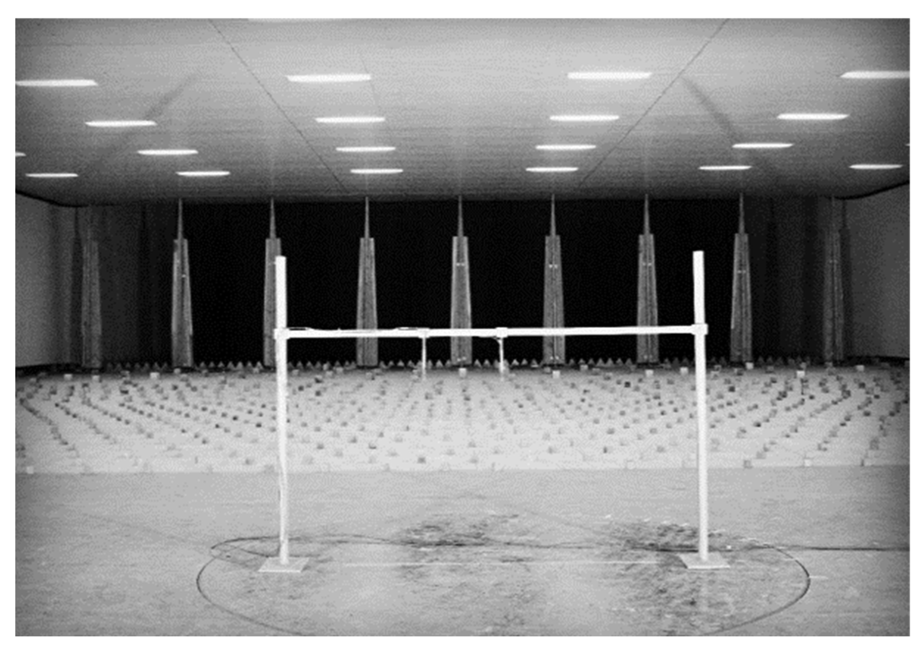
3. Experimental Setup

All the tests were conducted in a closed circuit-type boundary layer wind tunnel with a 22.5 (width) × 4.5 m (height) test section (XNJD-3). The traditional passive method was used to simulate the atmospheric boundary layer (i.e., upstream spires and the surface roughness on the wind tunnel floor). This study simulated three types of typical atmospheric boundary layer flows, where BL1, BL2, and BL3 denote the ground categories over open country terrain, suburban areas, and urban landforms, respectively (GB50009-2012, Architectural Industry Press of China, [36]).

Near the station where the measurements were to be taken, a rounded rod was fixed across the tunnel to support two Cobra Probes for lateral coherence tests. Cobra Probes are a type of wind speed measurement instrument that is frequently used in wind tunnel testing applications, where airflow conditions are intentionally and regularly changed. To increase the spacing combination number along with the lateral separation distance, seven observation points were established. The lateral separation between two adjacent points ranged from 0.05 to 0.45 m, with the greatest separation distance reaching 1.3 m. The effects of height on lateral correlation were investigated using three different observation points at 0.6 m, 0.9 m, and 1.2 m in height. Eleven measurement points were marked along the height in the vertical direction, with vertical spacing ranging from 0.03 to 1.62 m. The simulation and test of the turbulent wind field are shown in Figure 1. With point 1# taken as the starting point, the measuring point layout is shown in

Table 2. Layout of observation points (unit: m).

Probe Layout	1#	2#	3#	4#	5#	6#	7#	8#	9#	10#	11#
Lateral direction	0	0.45	0.6	0.65	0.73	0.95	1.3	-	-	-	-
Vertical direction	0	0.05	0.25	0.48	0.71	0.91	0.96	1.11	1.14	1.31	1.62

.

The flow field characteristics were calibrated by a Cobra Probe, and the wind fluctuations in three directions were measured simultaneously. A frequency response of more than 2000 Hz indicates that the Cobra Probe is stable and reliable when measuring turbulence. The wind velocity measurement uncertainty was about 0.18 m/s, the Cobra Probe was in good condition, and the test method was reasonable. The sampling frequency of turbulence in this study was 256 Hz, and the sampling period was 120 s, allowing the data length to be up to 30,720 and meeting the requirements of the coherence analysis [18,23,26,31,35]. The measured average wind velocity ($U_z$) and the turbulence intensities ($I_u$) of three incident turbulences at various heights are shown in Figure 2, where $z_0$ is the reference height, $U_0$ is the corresponding average wind velocity, and $z$ is the height of the probe. It is demonstrated that the exponent model can reasonably fit the profile of the average wind velocity. Because of the large size of the test section, a larger-scale wind field can be simulated, and the turbulence characteristics will be closer to atmospheric boundary layer turbulence, which has certain advantages in analyzing the turbulent spatial structure.

4. Results and Discussion

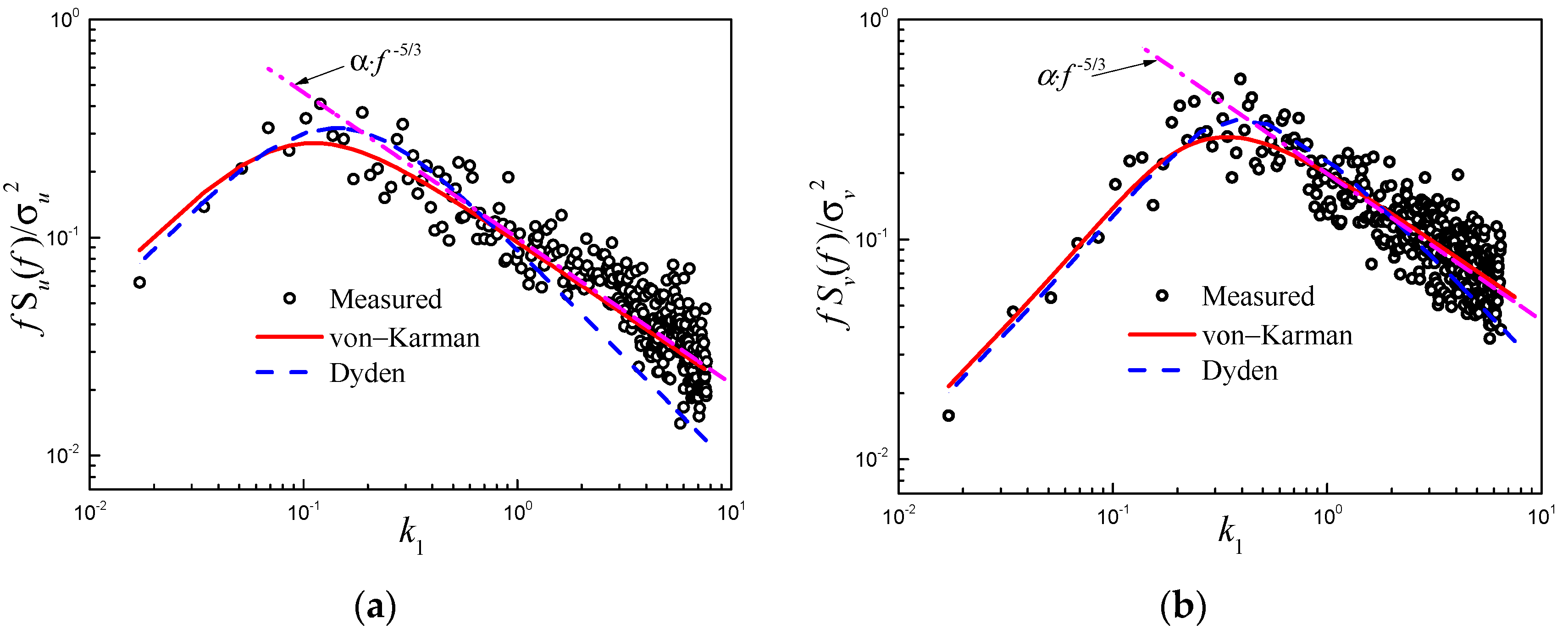
4.1. Statistical Parameters of Turbulence

The turbulent spectrum of three fluctuating velocity components of BL1 at $z=0.9\mathrm{m}$ is shown in Figure 3, where $S_u(f)$, $S_v(f)$, and $S_w(f)$ represent the spectral density of along-wind, lateral, and vertical wind fluctuation components. The measured spectrum agrees well with the theoretical models in the low-frequency range, which is consistent with other heights and turbulence flows. However, the fitting accuracy of the two theoretical models differs in the high-frequency range. The von Kármán spectrum model retains a good fitting accuracy, but the Dryden model has a higher attenuation rate at high frequencies, resulting in deviations from the test results. Figure 3 also shows the fitting result of the −5/3 exponential attenuation curve, which shows that the simpler −5/3 exponential attenuation theory can be used for description in the high-frequency attenuation area. This result demonstrates that theoretical simulation can better describe the spectral properties of passively stimulated turbulence, but there are some differences in the high-frequency inertial subregion and the dissipation region. The integral length scale can be obtained by fitting the von Kármán spectrum model using the nonlinear least square method.

Table 3. Statistical parameters of turbulence field.

Wind Field Type	Integral Length Scale			Turbulence Intensity
	Lu (m)	Lv (m)	Lw (m)	Iu (%)	Iv (%)	Iw (%)
BL1	1.216	0.376	0.301	12.8	10.7	8.4
BL2	1.158	0.351	0.268	20.8	18.2	16.7
BL3	1.027	0.324	0.232	27.1	22.1	18.3

displays the statistical parameters of the three turbulence fields.

According to the statistical turbulence parameters of several wind fields, the simulated wind field is basically consistent with the natural atmospheric turbulence, which can meet the research requirements. The length scales and the turbulence intensities for the three velocity components in Table 3 deviate slightly from the conditions typically seen in the atmospheric boundary layer. There are some limitations to the experimental observations due to the insufficiency of the commonly used wind tunnel [8,37]. For example, the turbulence intensity is different from the actual situation (i.e., I_u > I_v > I_w), and the difference between the three components is smaller than the field measurement result of the natural wind. This indicates that the wind velocity fluctuations of the w component of the simulated BL flows are stronger than those of the natural atmospheric boundary layer turbulence.

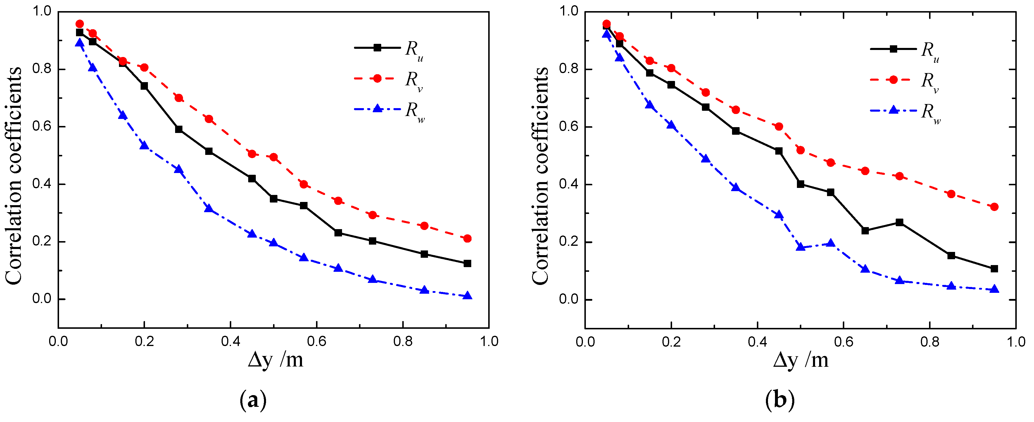
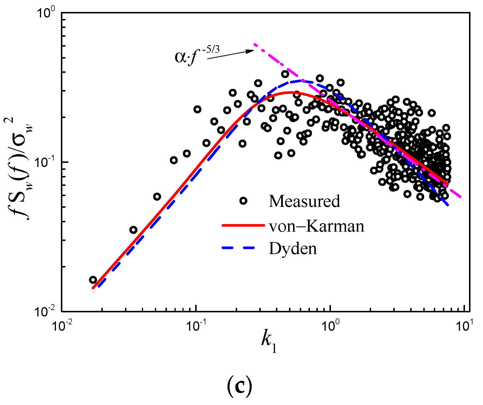
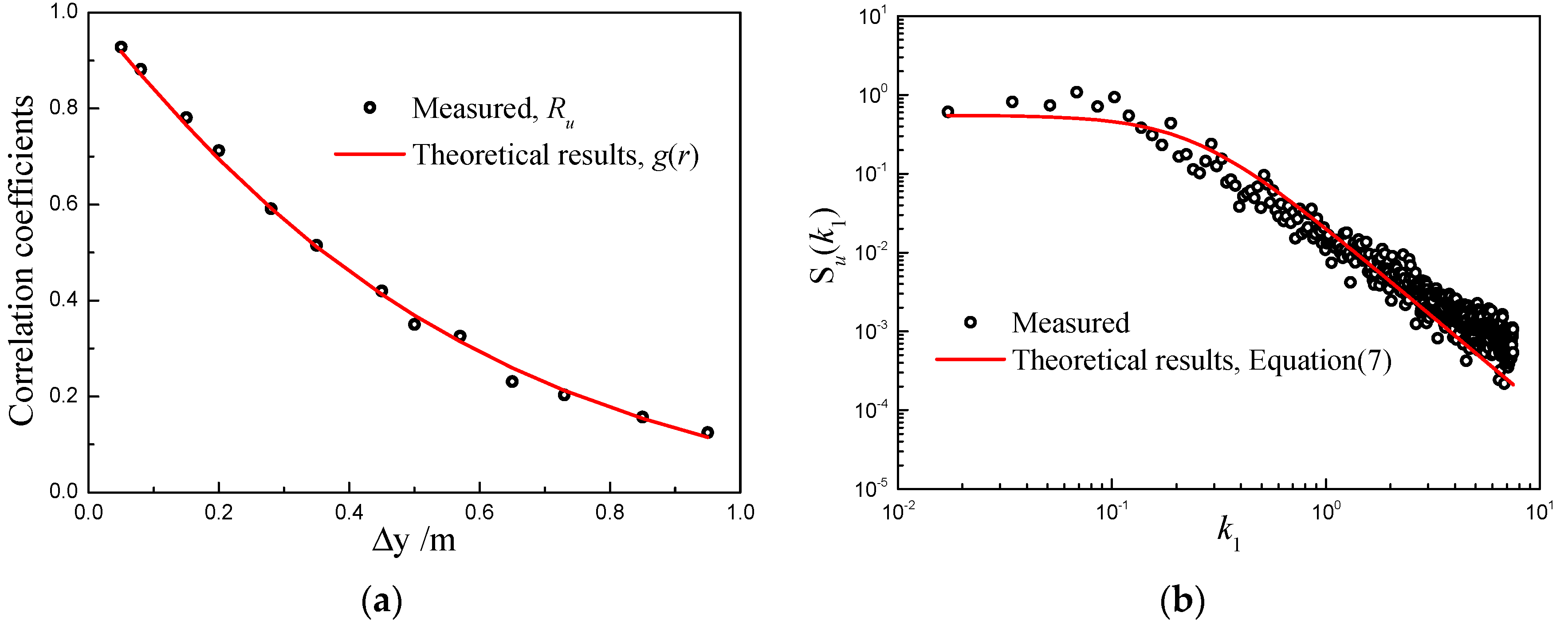
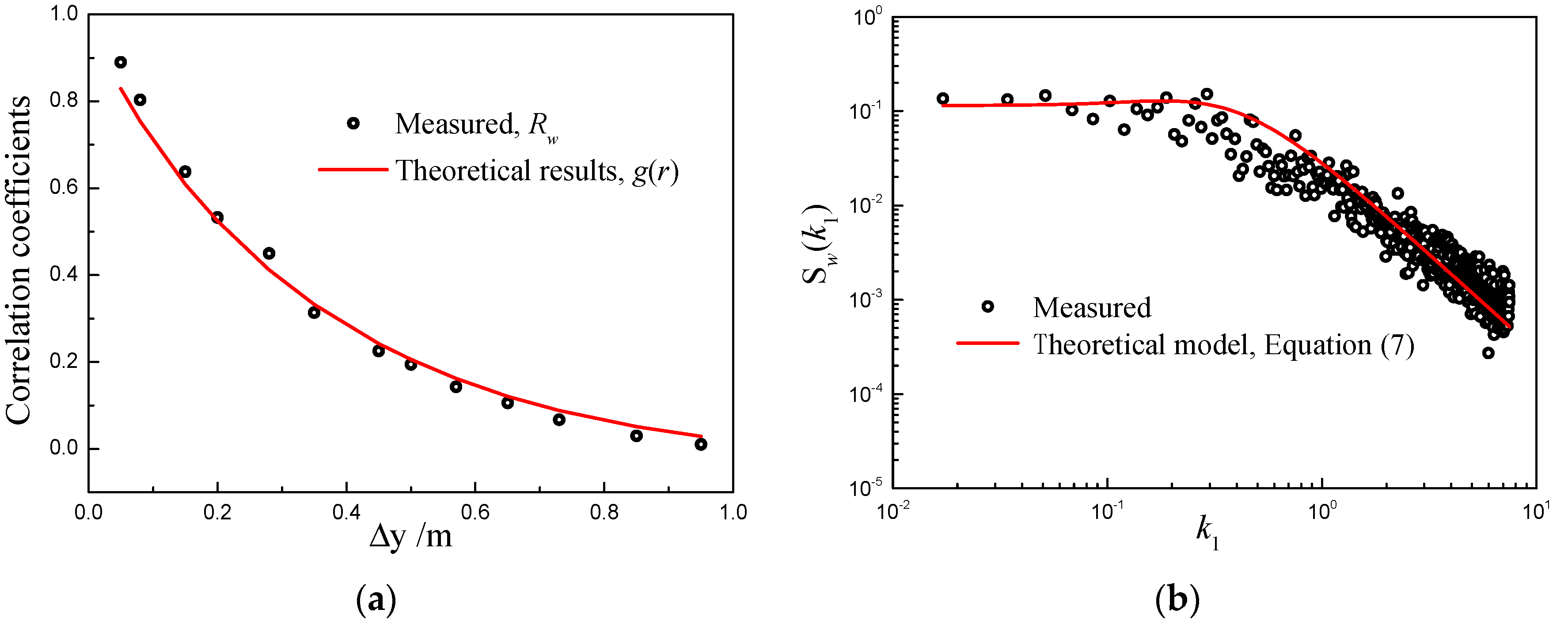
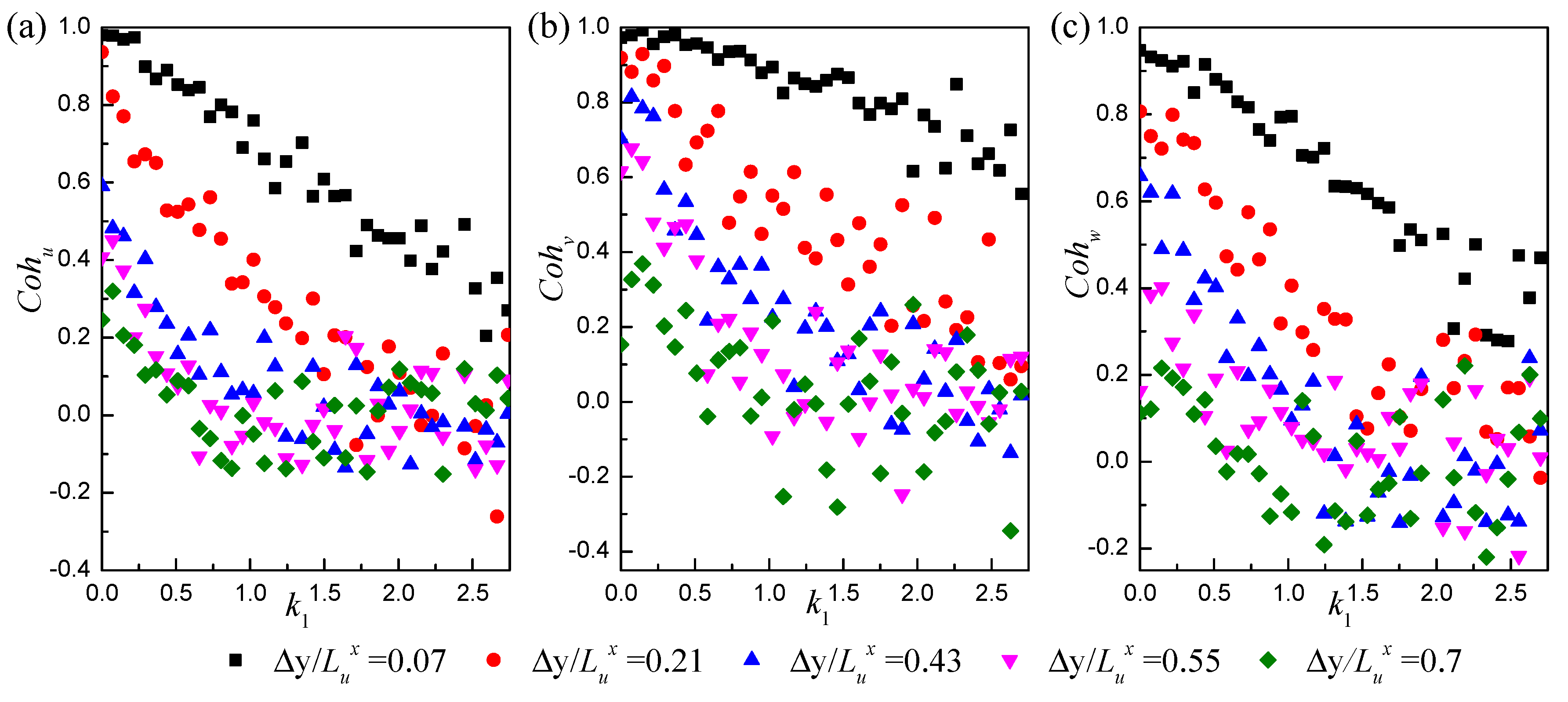
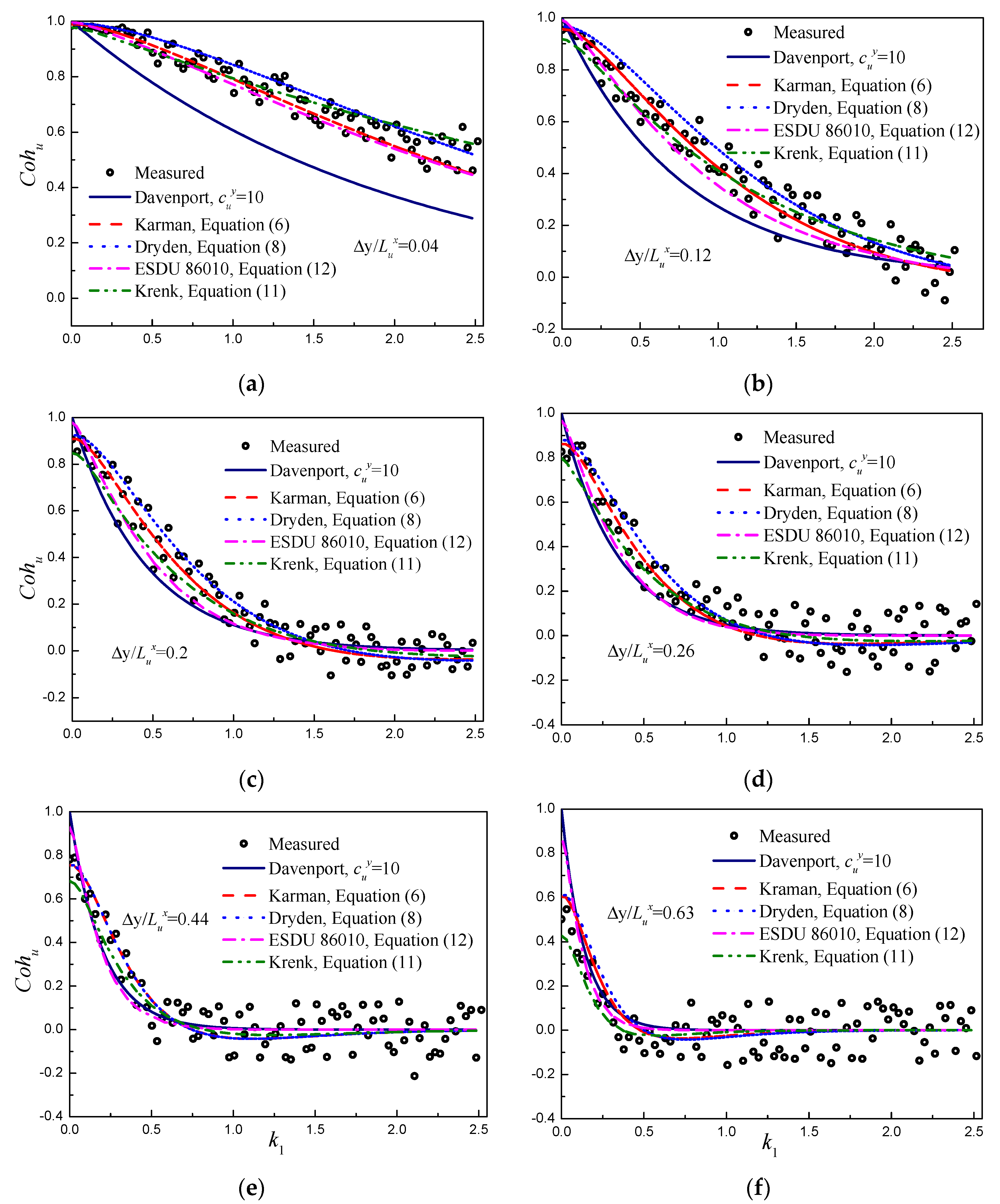
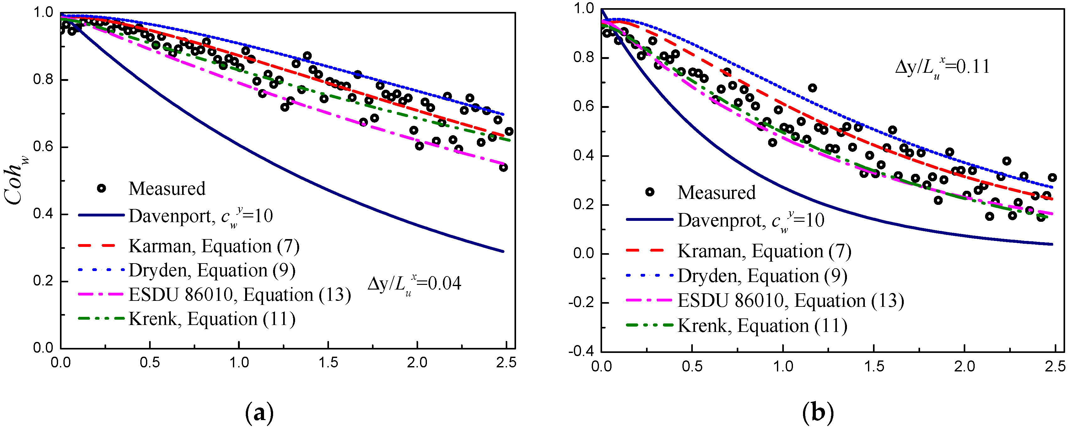
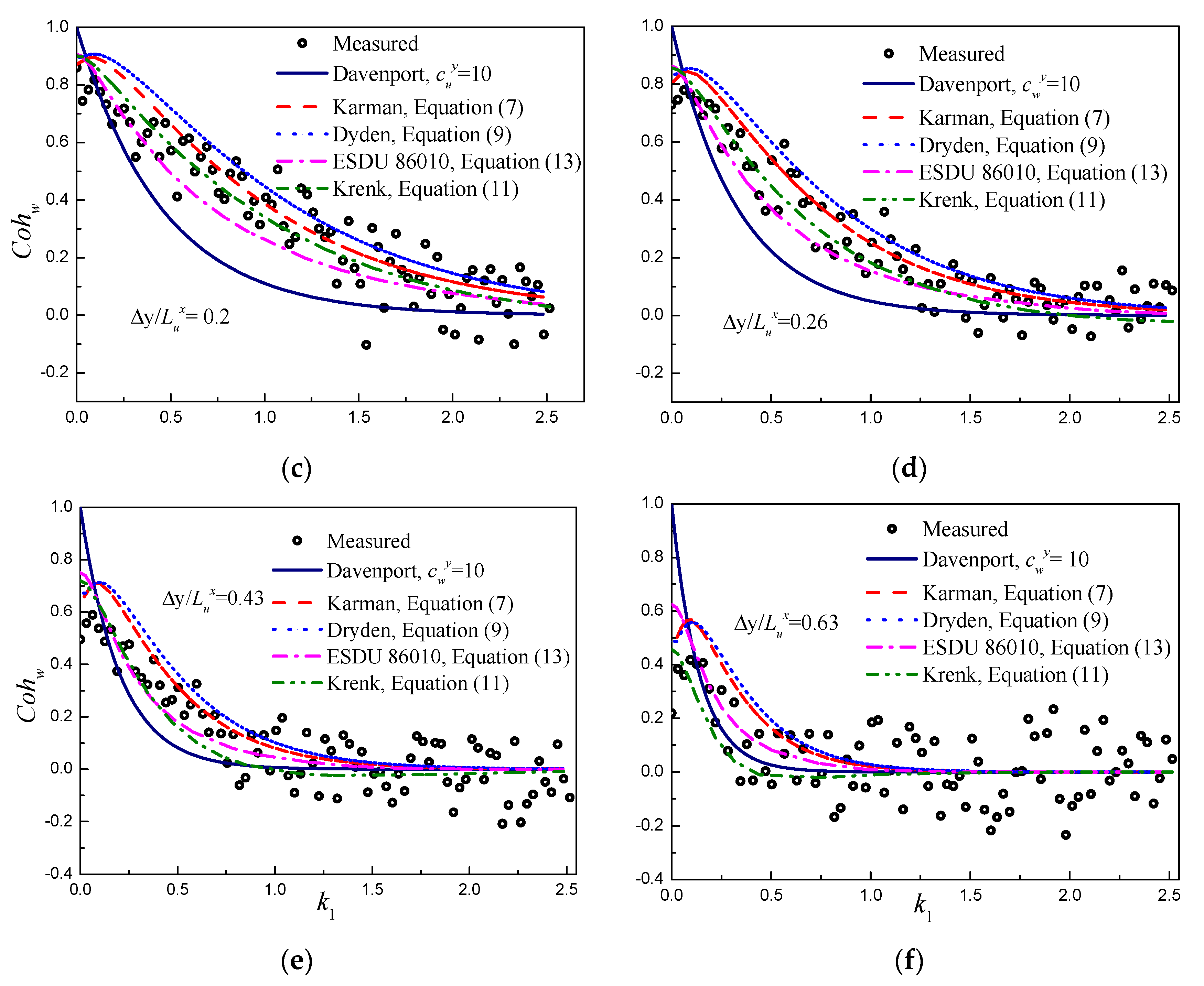
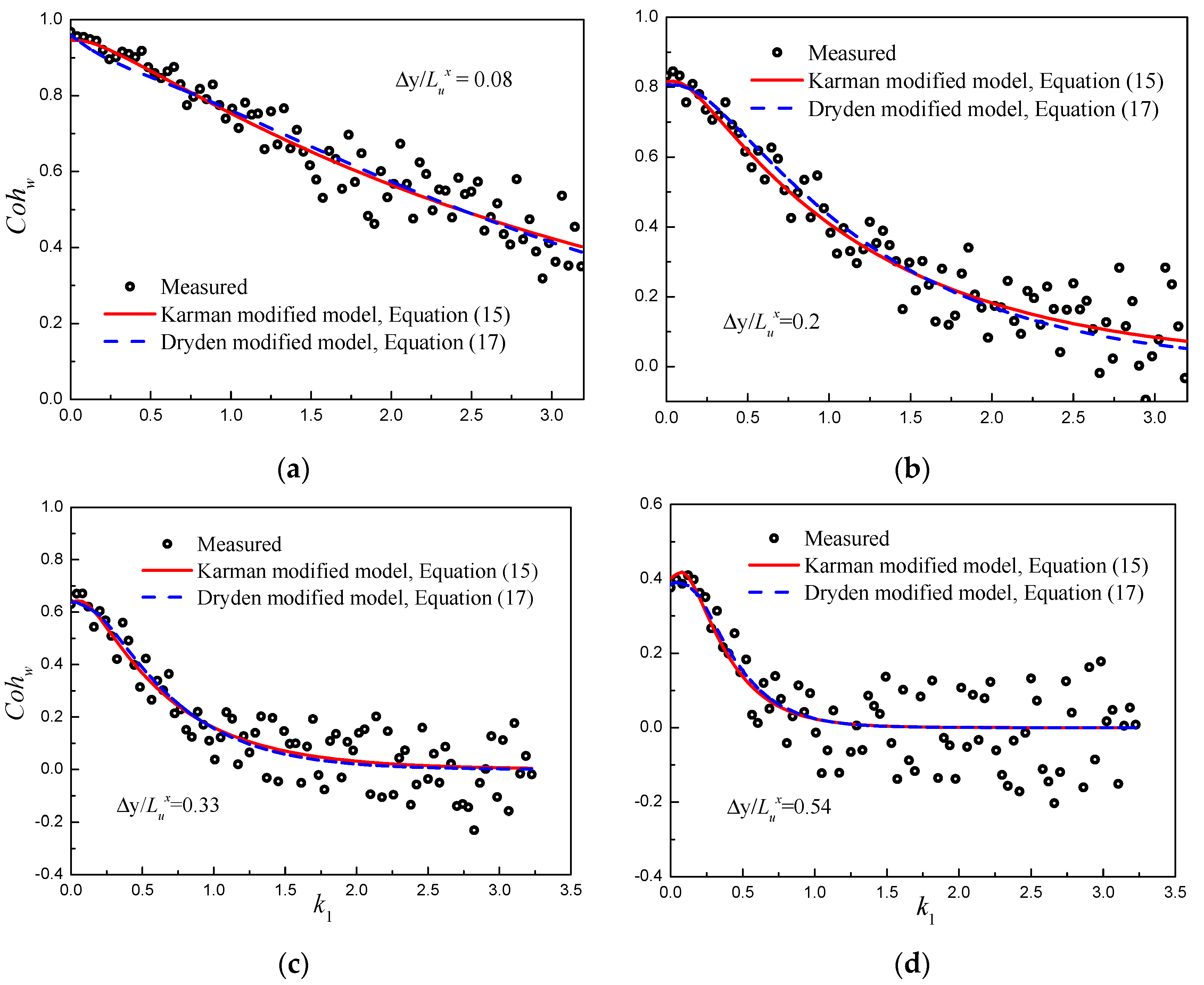
4.2. Lateral Spatial Structure

For lateral separation distances, the wind data were measured in the simulated turbulent boundary layer flows for nine cases. The time domain ensemble average shown in Equation (1) was used to calculate the correlation coefficients of different turbulent components, as shown in Figure 4.

For the simulated boundary layer turbulence, the lateral correlation of the three turbulent fluctuation components is $R_v>R_u>R_w$. According to the theoretical analysis of isotropic turbulence in the previous section, it can be seen that the turbulence satisfies 180° symmetry on the horizontal plane at the same height. For the horizontal and lateral distances, the $v$ component is equivalent to the along-wind correlation function, and the $u$ component and the $w$ component are the lateral correlation functions. The experimental data show that the along-wind turbulent component correlation is stronger than the vertical fluctuating wind component, indicating that the isotropic turbulence theory can describe the lateral correlation distribution of the stimulated turbulence. However, there are differences between the two results, and this difference becomes more significant as the turbulence intensity increases, indicating the influence of the nonisotropic turbulence component.

For transverse slender structures, such as long-span bridges, the spatial structure of the along-wind fluctuating component $u$ and vertical fluctuating component $w$ is generally more concerned. By fitting the cross-correlation coefficients ($g(r)$) measured in the BL1 wind field using the theoretical correlation function model [23,29,31], the parameters $n$ and $L$ were obtained, as shown in Figure 5.

In Figure 5a, the lateral correlation of the along-wind fluctuating wind component can be sufficiently described by homogeneous isotropic turbulence theory, and the fitting result is $n=0.614$ and $L=0.797$. The fitting result of the along-wind fluctuating wind spectrum deviates from the theoretical model, but the error is within acceptable limits, as illustrated in Figure 5b. The results show that homogeneous isotropic turbulence theory works well with a horizontal lateral spacing. It can be used to accurately describe the energy distribution and spatial structure of the fluctuating velocity components in the frequency domain.

Using the same method, the parameters $n$ and $L$ in the lateral correlation function of the vertical fluctuation component were fitted, as shown in Figure 6. The comparison results show that homogeneous isotropic turbulence theory can also be used to describe the lateral correlation of the $w$ component of the simulated atmospheric turbulence. The fitting result is $n=0.412$ and $L=0.523$. The fitting parameter $n$ is relatively close to the von Kármán spectrum model ($n=1/3$), and the length scale is the same as the result in Table 3, $L\approx 2L_u$, but there is a gap from the natural atmospheric turbulence. This result shows that the vertical component roughly satisfies the homogeneous isotropic assumption, and the fluctuating wind spectrum agrees well with the von Kármán spectrum model. Although the lateral correlation function differs from natural atmospheric turbulence, the error is within engineering practice’s acceptable range.

In summary, although the statistical parameters of the wind tunnel-simulated turbulent wind field are different from the theoretical results and natural atmospheric turbulence, the lateral spatial structure can still be described approximately by isotropic turbulence theory. The coherence function, which is one of the fundamental functions for calculating the wind-induced response of wind-sensitive structures, is also different from the theoretical derivation or the field-measured value, and some targeted corrections are required. Relevant studies [16,17,19,37,38] have shown that many factors in natural atmospheric turbulence will affect the coherence function, such as turbulence, the integral scale, and the vertical wind speed gradient. Representative lateral coherences are shown in Figure 7, where the coherences for $z=0.6\mathrm{m}$ are plotted against $k_1$.

According to the results of the measured coherence function, some basic characteristics of the lateral coherence function of the simulated atmospheric turbulence can be summarized. To begin with, the lateral coherence of the simulated turbulent wind field differs from isotropic turbulence theory and the field-measured results of natural atmospheric turbulence, both of which can be considered to approximate the horizontal homogeneous isotropic assumption. Second, the lateral distance and the turbulence integral scale have the greatest influence on the lateral coherence. The type of wind field and the height of the measuring point above the ground will have an effect on the attenuation rate, but only a minor effect on the overall distribution trend of the coherence function, which can be ignored in engineering applications. To further verify the correlation between the experimentally measured coherence and the theoretical result, Figure 8 shows the fitting conditions of the existing models.

For the coherence with a measured value that is too small, the discreteness is large and the noise interference is strong, meaning the analysis significance is minor. For this reason, this investigation requires the selected coherence function $Co{h}_u>0.1$. The fitting results show that when the dimensionless distance is $0.04\le \Delta y/L_u^x\le 0.63$, the measured data are in good agreement with the theoretical models, indicating that the experimental data and the degrees of freedom in the calculation are reasonable. The isotropic turbulence theory-derived Dryden model and von Kármán model can sufficiently describe the coherence of the along-wind component and have high fitting accuracy under all spacing combinations. This demonstrates that the along-wind fluctuation component can be accurately described by the theoretical coherence function model under a lateral spacing. Based on the assumption of horizontal homogeneous isotropic turbulence, the correlation of the along-wind fluctuating velocity component at any lateral spacing can be sufficiently described for the simulated turbulence field, which simplifies the analysis of the structure’s wind resistance performance.

In Figure 9, the value of the low-frequency region and the attenuation rate of the vertical component coherence function are different from those of the along-wind component. Davenport’s exponential experience model is no longer applicable. Especially when $\Delta y/L_u^x\le 0.26$, the fitting result is seriously smaller than the measured data, and the attenuation law in the low-frequency region cannot be accurately described. When $\Delta y/L_u^x\le 0.26$, the Dryden and von Kármán coherence function model can describe the distribution trend of the vertical component coherence function, but the fitting result in the low-frequency region is higher than the measured data. When $\Delta y/L_u^x>0.26$, the fitting deviation gradually becomes significant as the distance increases.

The fitting results of the coherence function show that the vertical fluctuating component is significantly affected by the shear stress of the boundary layer, resulting in the rotation or stretching of the vortex, meaning that the turbulent spatial structure under a horizontal lateral spacing gradually becomes “nonisotropic”. Given the importance of the coherence of the vertical component in wind-induced vibration analysis, and the fact that the accuracy of the existing empirical or theoretical model cannot meet the requirements of engineering practice, some improvements are required.

Based on the theory of isotropic turbulence, scholars have modified the lateral coherence function model of grid turbulence to describe the influence of nonisotropic components on the spatial structure of turbulence. Although the 3D structure of atmospheric boundary layer turbulence is more complicated than grid turbulence, it is a simple and effective method for improving the existing theoretical model based on the horizontal isotropic turbulence assumption. This study examined the stretching effect of nonisotropic turbulence components on vortices of various scales using correction of the turbulence integral scale and wave number and attempted to extend this correction method to atmospheric boundary layer turbulence. Based on the von Kármán coherence model, the modified model form of the vertical component is

$$Co{h}_w\left(k_1,\Delta y\right)=\frac{2^{1+\zeta /2}}{\Gamma \left(-\zeta /2\right)}\cdot \left[{\eta }_{\chi }{}^{-\zeta /2}{K}_{\zeta /2}\left({\eta }_{\chi }\right)-\frac{{\eta }_{\chi }{}^{1-\zeta /2}{K}_{1+\zeta /2}({\eta }_{\chi })}{B_K}\right]$$

(15)

$$\begin{gathered} {\eta }_{\chi }=\frac{\Delta y\beta }{a_1{L}_u^x}\cdot \sqrt{1+{(2\pi k_1{a}_1{L}_u^x/\beta )}^{b_1}} \\ {B}_K=1+\frac{8}{3}\cdot {(2\pi k_1{a}_1{L}_u^x/\beta )}^{b_1} \end{gathered}$$

(16)

Using a similar definition, a modified model based on the Dryden theoretical model can be obtained:

$$Co{h}_w\left(k_1,\Delta y\right)={\theta }_{\chi }{K}_1\left({\theta }_{\chi }\right)-\frac{{\theta }_{\chi }{}^2}{B_D}{K}_0\left({\theta }_{\chi }\right)$$

(17)

In the above formula, the expression of the modified parameter is as follows:

$$\begin{gathered} {\theta }_{\chi }=\frac{\Delta y}{a_2{L}_u^x}\cdot \sqrt{1+{(2\pi k_1{a}_2{L}_u^x)}^{b_2}} \\ {B}_D=1+3\cdot {(2\pi k_1{a}_2{L}_u^x)}^{b_2} \end{gathered}$$

(18)

When fitting the experimental data, the nonlinear least square method can be used to obtain the undetermined parameters. The fitting parameters of the improved model are shown in

Table 4. Fitting parameters of different coherence models.

Wind Field Type		Von Kármán Model		Dryden Model
	$\mathit{z}(\mathbf{m})$	${\mathit{a}}_1$	${\mathit{b}}_1$	${\mathit{a}}_2$	${\mathit{b}}_2$
BL1	0.6	0.489	1.535	0.512	1.978
	0.9	0.493	1.52	0.568	2.013
	1.2	0.527	1.587	0.582	2.075
BL2	0.6	0.491	1.591	0.547	1.993
	0.9	0.513	1.632	0.528	2.043
	1.2	0.524	1.643	0.574	2.123
BL3	0.6	0.466	1.665	0.533	1.96
	0.9	0.507	1.653	0.577	2.01
	1.2	0.52	1.727	0.583	2.085

, and the fitting results are shown in Figure 10, after fitting 189 distance combinations under three types of turbulent wind fields

According to the fitting results of the vertical component coherence function in the BL3 turbulent wind field at z = 0.9 m, it can be found that the modified models are in good agreement with the measured results. The improved von Kármán and Dryden theoretical models can describe the vertical component coherence function distribution at any interval and correct the problem of overestimating the value of the low-frequency region at large intervals. Table 4’s coefficients take into account all influencing factors and average the fitting results for each measurement height and spacing combination. Each parameter varies with the wind field and measurement height, but the distribution law is obvious and can be approximated as a constant. In the modified von Kármán model (Equation (15)), the coefficients are recommended to be $a_1=0.5$ and $b_1=1.62$; the correction coefficients in the Dryden correction model (Equation (17)) are recommended to be $a_2=0.56$ and $b_2=2$.

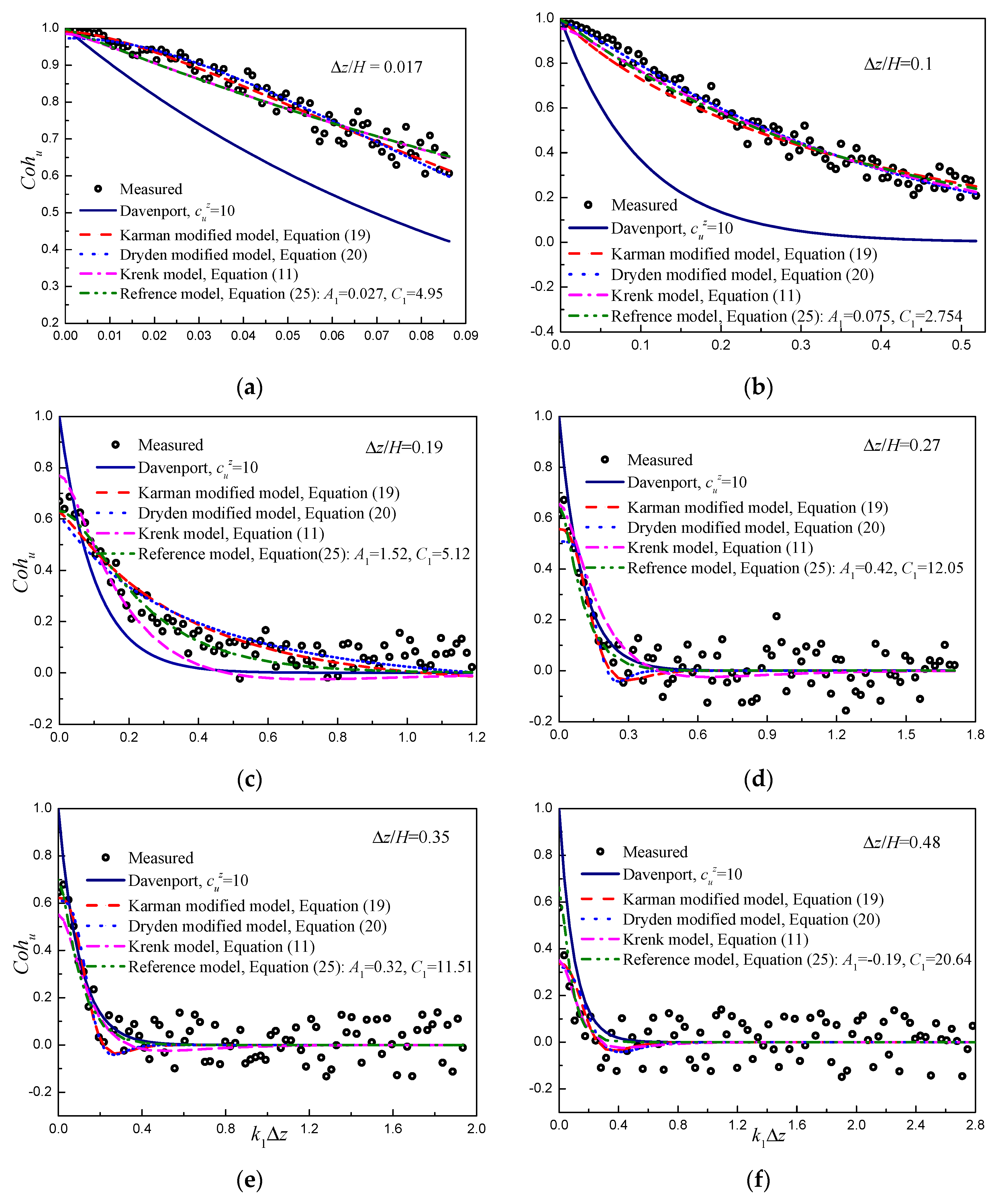
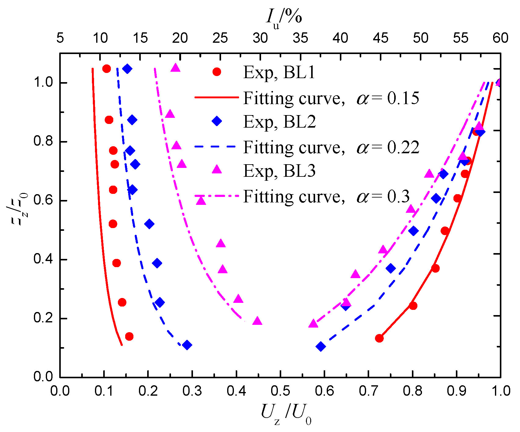
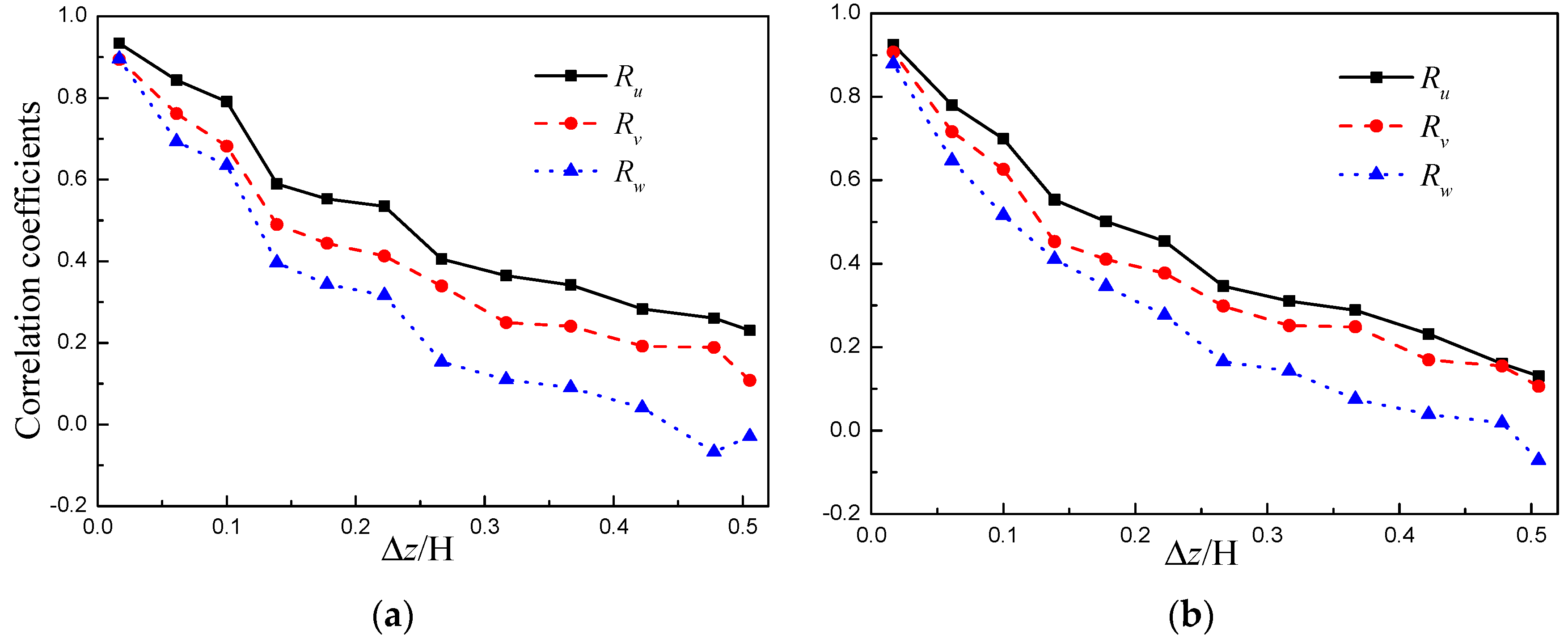
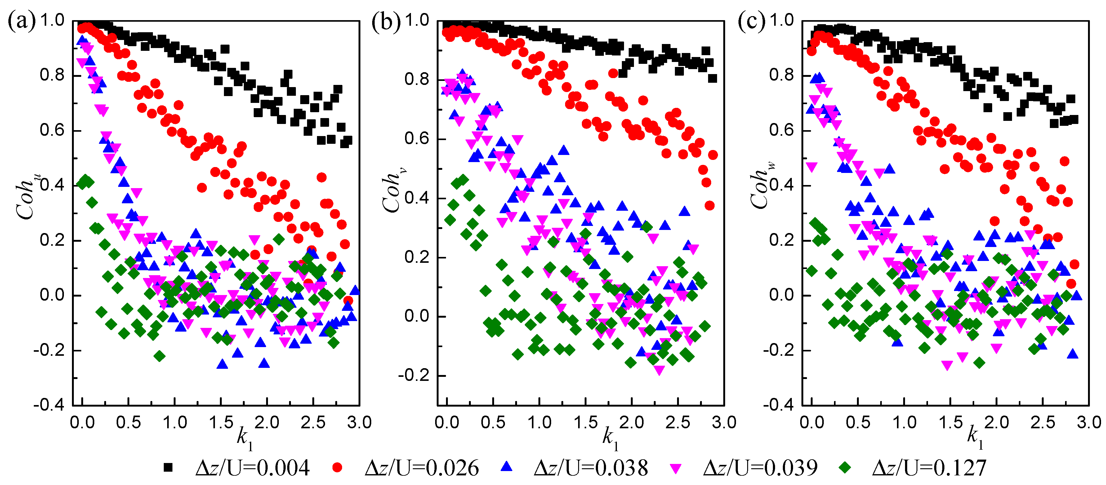
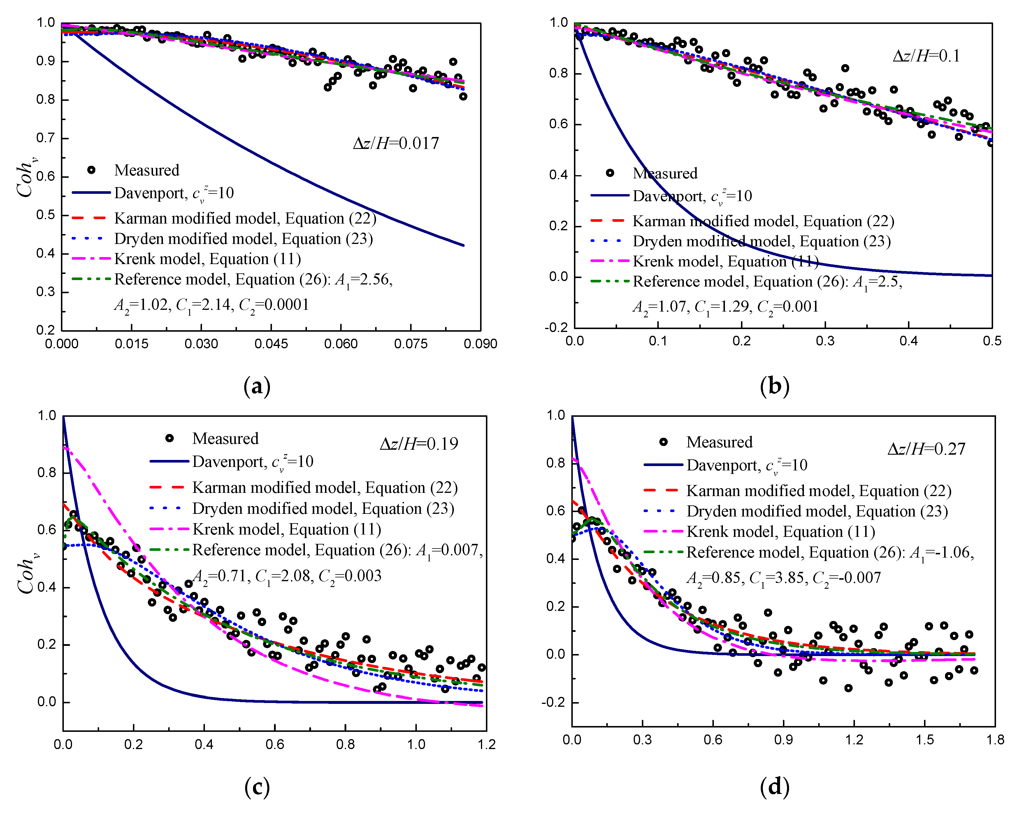
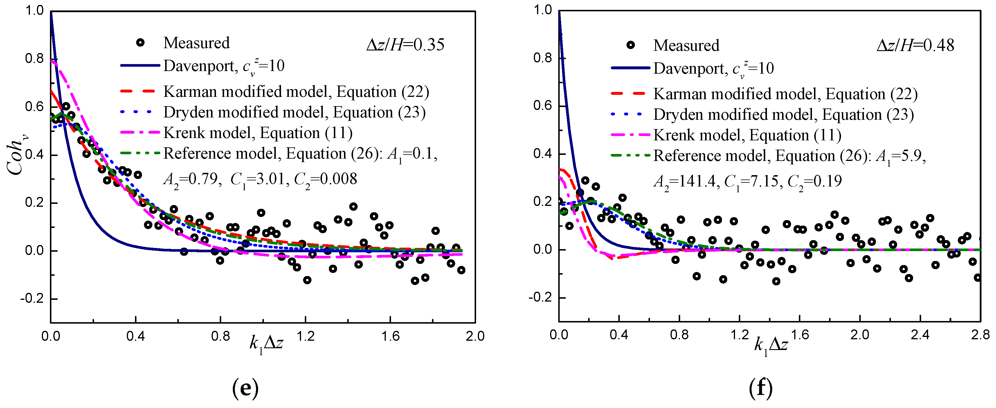
4.3. Vertical Spatial Structure

Due to the complex vertical spatial structure of the natural shear flow, isotropic turbulence theory is no longer applicable in the vertical direction. However, an in-depth study of the vertical spatial structure of atmospheric turbulence is an important direction for the refined analysis of high-rise buildings’ wind resistance performance. Because the vertical spatial structure of atmospheric turbulence is so complicated, the theoretical derivation is still difficult to solve. The primary research method is still to collect a large amount of data via field measurements of natural atmospheres or wind tunnel tests, followed by fitting to obtain an approximate empirical model. This study obtained the spatial correlation of 55 vertical spacing combinations in each wind field by real-time measurement of fluctuating wind time history data at different heights. According to the definition of Equation (1), the cross-correlation coefficients under different spacing combinations were obtained, and the variation trend of the correlation coefficient with the dimensionless spacing $\Delta z/H$ is shown in Figure 11, where $H$ is the height of the highest collection point.

The relationship between the vertical correlations of each velocity component is $R_u>R_v>R_w$, which is quite different from the horizontal lateral correlation. The vertical correlation coefficients of the three types of simulated turbulent wind fields are the same with the change in the distance, and the values are relatively close. This demonstrates that the type of ground roughness has little effect on the vertical correlation of the turbulence field, which is a key feature of simulating atmospheric turbulence. The partial spacing combinations were used as examples in the frequency domain to demonstrate the influence of vertical distance on the coherence of each turbulence component, as shown in Figure 12.

The results show that the vertical coherence function is not only related to wind field factors such as the turbulence intensity, length scale, and wave number but also the average height of the measurement point combination, which is mainly reflected by the average wind speed at two heights, namely, $U=(U_{z_1}+U_{z_2})/2$. The overall distribution trend of the vertical coherence function with the wave number is similar to the lateral coherence. As the distance and wave number increase, the coherence function gradually decreases, and the attenuation rate increases continuously.

Following extensive comparative analysis, it was discovered that there is a special relationship between the vertical coherence function and parameter $\Delta z/U$. In Figure 12, two coherence curves with approximate coefficients $\Delta z/U$ can be found, in which the distribution characteristics are almost the same. Therefore, it may be concluded that if the values of $\Delta z/U$ are close, the two coherences can be regarded as similar. For any vertical spacing, the vertical coherence is basically inversely proportional to the size $\Delta z/U$. That is, if the value $\Delta z/U$ is smaller, the correlation of the two points will be stronger and the decay rate of coherences will be relatively small. As a result, despite the fact that the spatial structure of turbulence in the vertical direction is complex and has many influencing factors, the coherences of other arbitrary heights can be roughly and quickly deduced based on the ratio $\Delta z/U$ after measuring a few wind velocity data, which is useful in engineering practice.

Considering that atmospheric turbulence has a complex vertical spatial structure, which is affected by many factors, it is difficult to use theoretical isotropic turbulence models to describe it completely. Because the vertical coherence of fluctuating wind is a fundamental equation necessary for calculating the wind-induced response of high-rise buildings, the empirical coherence function model is typically obtained by fitting a large amount of measured data. The modified Krenk model (Equation (11)), the ESDU 86010 simplified model (Equations (12) and (13)), and Davenport’s model (Equation (14)) are the most commonly used coherence function models. Based on extensive research on the spatial structure of atmospheric turbulence, it has been discovered that existing models have some shortcomings in describing the vertical spatial structure of the natural shear flow. Therefore, this study attempted to make some amendments to those existing coherence function models.

In structural wind engineering, the vertical coherence function of the along-wind and lateral components is the focus of attention. In order to conduct a comparative analysis, we referred to the above correction method to improve the theoretical models of von Kármán and Dryden and then obtained the undetermined parameters by fitting the experimental data. The vertical coherence model expression of the along-wind component is

$$Co{h}_u\left(k_1,\Delta y\right)=\frac{2^{1+\zeta /2}}{\Gamma \left(-\zeta /2\right)}\cdot \left[{\eta }_{\chi }{}^{-\zeta /2}{K}_{\zeta /2}\left({\eta }_{\chi }\right)-\frac{{\eta }_{\chi }{}^{1-\zeta /2}{K}_{1+\zeta /2}({\eta }_{\chi })}{2}\right]$$

(19)

$$Co{h}_u\left(k_1,\Delta y\right)={\theta }_{\chi }{K}_1\left({\theta }_{\chi }\right)-\frac{{\theta }_{\chi }{}^2}{2}{K}_0\left({\theta }_{\chi }\right)$$

(20)

where the correction coefficients ${\eta }_{\chi }$ and ${\theta }_{\chi }$ are as follows:

$$\begin{gathered} {\eta }_{\chi }=\frac{\Delta y\beta }{a_1{L}_u^x}\cdot \sqrt{1+{[(2\pi /\beta )\cdot (a_1{k}_1{L}_u^x)]}^{b_1}} \\ {\theta }_{\chi }=\frac{\Delta y}{a_2{L}_u^x}\cdot \sqrt{1+{(2\pi )}^2\cdot {[{(k_{1}U)}^{\chi }(\frac{a_2{L}_u^x}{U})]}^2} \end{gathered}$$

(21)

The vertical coherence correction model expression of the lateral component is

$$Co{h}_v\left(k_1,\Delta y\right)=\frac{2^{1+\zeta /2}}{\Gamma \left(-\zeta /2\right)}\cdot \left[{\eta }_{\chi }{}^{-\zeta /2}{K}_{\zeta /2}\left({\eta }_{\chi }\right)+\frac{{\upsilon }_{\chi }{}^2{\eta }_{\chi }{}^{1-\zeta /2}{K}_{1+\zeta /2}({\eta }_{\chi })}{B_{\chi }}\right]$$

(22)

$$Co{h}_v\left(k_1,\Delta y\right)=\frac{2^{1+\zeta /2}}{\Gamma \left(-\zeta /2\right)}\cdot \left[{\eta }_{\chi }{}^{-\zeta /2}{K}_{\zeta /2}\left({\eta }_{\chi }\right)+\frac{{\upsilon }_{\chi }{}^2{\eta }_{\chi }{}^{1-\zeta /2}{K}_{1+\zeta /2}({\eta }_{\chi })}{B_{\chi }}\right]$$

(23)

where $B_{\chi }$, $B_D$, and ${\upsilon }_{\chi }$ are correction terms:

$$\begin{gathered} B_K=1+\frac{8}{3}\cdot {(2\pi k_1{\alpha }_1{L}_u^x/\beta )}^{b_1} \\ {B}_D=1+3\cdot {(2\pi k_1{\alpha }_2{L}_u^x)}^{b_2} \\ {\upsilon }_{\chi }=2\pi a_1{L}_u^x{k}_1\mathrm{or}{\upsilon }_{\chi }=2\pi a_2{L}_u^x{k}_1 \end{gathered}$$

(24)

At the same time, the model is verified with reference to an empirical model of the vertical coherence function proposed by Huang [26], and its expression is as follows:

$$Co{h}_u(k_1,\Delta z)=\exp (-C_1{k}_1\Delta z\cdot \sqrt{1+{(\frac{A_1}{f})}^2})$$

(25)

$$Co{h}_v(k_1,\Delta z)=A_2\cdot (1-\frac{C_2}{k_1\Delta z\cdot \sqrt{1+{(A_1/f)}^2}})\exp (-C_1{k}_1\Delta z\cdot \sqrt{1+{(A_1/f)}^2})$$

(26)

where $A_1$, $A_2$, $C_1$, and $C_2$ are undetermined parameters. Taking the selected vertical spacing combinations as an example, Figure 13 shows the coherence function fitting of the along-wind component in the BL1 wind field.

According to the fitting results, it can be found that several types of coherence function models can roughly reflect the vertical coherence function of the along-wind component. However, when the distance is small, the Davenport coherence model is significantly lower than the measured data, and when the distance is large, there is a deficiency of overestimating the low-frequency value. The undecided parameters for the modified vertical coherence model will vary with the vertical spacing, integration scale, average wind speed, and height above ground, but the fluctuation range is generally small. To make practical engineering applications easier, the fitting results can be approximated by an average value. For the vertical coherence function of the along-wind component, the modified von Kármán model takes $a_1=0.678$ and $b_1=1.175$, and the modified Dryden model takes $a_2=0.72$ and $b_2=2.293$. The reference model has a simple structure and high fitting accuracy, and its undetermined coefficients can be obtained by fitting experimental data.

Using a similar method, Figure 14 shows the fitting result of the vertical coherence function of the lateral fluctuation component. The fitting results show that both the improved models (Equations (22) and (23)) and the reference model (Equation (26)) can accurately describe the vertical coherence distribution trend. In comparison, the modified Dryden model better describes the variation of the lateral component’s vertical coherence with the frequency and vertical spacing. The fitting parameters can be approximately averaged at different distances, which can meet the requirements of engineering applications. Among them, the undetermined parameters of the modified von Kármán model are $a_1=0.61$ and $b_1=1.584$, and the undetermined parameters of the modified Dryden model are $a_2=0.329$ and $b_2=2.205$. The reference model has a simple structure and clear physical meaning; it can sufficiently describe the “turn around” phenomenon of the vertical coherence function of the lateral fluctuation component in the low-frequency region, and its undetermined parameter fitting method has been presented in the relevant literature [37]. The Krenk model and Davenport model can roughly reflect the vertical coherence distribution under different vertical spacings, but the fitting accuracy has some flaws and needs to be improved further.

5. Conclusions

In this study, based on the analysis of turbulence theory, the lateral and vertical spatial structures of atmospheric turbulence passively simulated by a wind tunnel were discussed. The following conclusions can be drawn from this study:

(1)

The passively simulated atmospheric turbulence can be approximately regarded as conforming to the assumption of horizontal average isotropic turbulence, but the vertical turbulence component is more significantly disturbed by the nonisotropic component and cannot be ignored.

(2)

Isotropic turbulence theory sufficiently describes the horizontal and lateral spatial structures of the along-wind turbulence component, but the vertical component deviates slightly. The modified theoretical coherence model can better describe the distribution of the lateral coherence of the vertical component due to improvements to the theoretical coherence model.

(3)

The vertical spatial structure that passively simulated atmospheric turbulence was discussed. Due to the influence of turbulent friction, isotropic turbulence theory cannot accurately describe the vertical spatial structure of atmospheric boundary layer turbulence simulated by wind tunnels. Through the improvement of the theoretical model, a modified vertical coherence model of different turbulence velocity components was obtained.

References

1. von Kármán, T. Progress in the statistical theory of turbulence. Proc. Natl. Acad. Sci. USA 1948, 34, 530–539. [Google Scholar] [CrossRef] [Green Version]
2. Davenport, A.G. Rationale for determining design wind velocities. J. Struct. Div. 1960, 86, 39–68. [Google Scholar] [CrossRef]
3. Panofsky, H.A.; Dutton, J.A. Atmospheric Turbulence; John Wiley & Sons: New York, NY, USA, 1984. [Google Scholar]
4. Hunt, J.C.R.; Carruthers, D.J. Rapid distortion theory and the ‘problems’ of turbulence. J. Fluid Mech. 1990, 212, 497–532. [Google Scholar] [CrossRef] [Green Version]
5. Kaimal, J.C.; Wyngaard, J.C.; Izumi, Y.; Cote, O.R. Spectral characteristics of surface-layer turbulence. Q. J. R. Meteorol. Soc. 1972, 98, 563–589. [Google Scholar] [CrossRef]
6. Solari, G. Mathematical model to predict 3-D wind loading on buildings. J. Eng. Mech. 1985, 111, 254–276. [Google Scholar] [CrossRef]
7. Kareem, A. Structure of wind field over the ocean. In Proceedings of the International Workshop on Offshore Winds and Icing, Halifax, NS, Canada, 7–11 October 1986; Environment Canada, Atmospheric Service: Toronto, ON, Canada, 1986. [Google Scholar]
8. Mann, J. The spatial structure of neutral atmospheric surface-layer turbulence. J. Fluid Mech. 1994, 273, 141–168. [Google Scholar] [CrossRef]
9. Simiu, E.; Scanlan, R.H. Wind Effects on Structures: Fundamentals and Applications to Design, 3rd ed.; John Wiley & Sons: New York, NY, USA, 1996. [Google Scholar]
10. Li, Q.S.; Zhi, L.; Fei, H. Boundary layer wind structure from observations on a 325 m tower. J. Wind Eng. Indust. Aerodyn. 2010, 98, 818–832. [Google Scholar] [CrossRef]
11. Cao, S.Y.; Tamura, Y.; Kikuchi, N.; Saito, M.; Nakayama, I.; Matsuzaki, Y. A case study of gust factor of a strong typhoon. J. Wind Eng. Indust. Aerodyn. 2015, 138, 52–60. [Google Scholar] [CrossRef]
12. Fenerci, A.; Oiseth, O.; Ronnquist, A. Long-term monitoring of wind field characteristics and dynamic response of a long-span suspension bridge in complex terrain. Eng. Struct. 2017, 147, 269–284. [Google Scholar] [CrossRef]
13. Zhao, L.; Cui, W.; Ge, Y.J. Measurement, modeling and simulation of wind turbulence in typhoon outer region. J. Wind Eng. Indust. Aerodyn. 2019, 195, 104021. [Google Scholar] [CrossRef]
14. Tao, T.Y.; Xu, Y.L.; Huang, Z.F.; Zhan, S.; Wang, H. Buffeting analysis of long-span bridges under typhoon winds with time-varying spectra and coherences. J. Struct. Eng. 2020, 146, 04020255. [Google Scholar] [CrossRef]
15. Fang, G.S.; Pang, W.C.; Zhao, L.; Cui, W. Extreme typhoon wind speed mapping for coastal region of China: Geographically weighted regression–based circular subregion algorithm. J. Struct. Eng. 2021, 147, 04021146. [Google Scholar] [CrossRef]
16. Roberts, J.B.; Surry, D. Coherence of grid-generated turbulence. J. Eng. Mech. Div. 1973, 99, 1227–1245. [Google Scholar] [CrossRef]
17. Maronga, B.; Li, D. An investigation of the grid sensitivity in large-eddy simulations of the stable boundary layer. Bound. Layer Meteorol. 2021, 180, 1–23. [Google Scholar] [CrossRef]
18. Kristensen, L.; Jensen, N.O. Lateral coherence in isotropic turbulence and in the natural wind. Bound. Layer Meteorol. 1979, 17, 353–373. [Google Scholar] [CrossRef]
19. Townsend, A.A. The Structure of Turbulent Shear Flow, 2nd ed.; Cambridge University Press: London, UK, 1976. [Google Scholar]
20. Emeis, S. Observational techniques to assist the coupling of CWE/CFD models and meso-scale meteorological models. J. Wind Eng. Indust. Aerodyn. 2015, 144, 24–30. [Google Scholar] [CrossRef]
21. Arolla, S.K.; Durbin, P.A. LES of spatially developing turbulent boundary layer over a concave surface. J. Turbul. 2015, 16, 81–99. [Google Scholar] [CrossRef] [Green Version]
22. Fernando, H.J.S.; Weil, J.C. Whither the stable boundary layer? A shift in the research agenda. Am. Meteorol. Soc. 2010, 91, 1475–1484. [Google Scholar] [CrossRef] [Green Version]
23. Zhong, Y.Z.; Li, M.S.; Ma, C.M. Aerodynamic admittance of truss girder in homogeneous turbulence. J. Wind Eng. Indust. Aerodyn. 2018, 172, 152–163. [Google Scholar] [CrossRef]
24. Huo, T.; Tong, L.W.; Mashiri, F.R. Turbulent wind field simulation of wind turbine structures with consideration of the effect of rotating blades. Adv. Steel Constr. 2019, 15, 82–92. [Google Scholar] [CrossRef]
25. Cao, S.Y.; Nishi, A.; Hirano, K.; Ozono, S.; Miyagi, H.; Kikugawa, H.; Matsuda, Y.; Wakasugi, Y. An actively controlled wind tunnel and its application to the reproduction of the atmospheric boundary layer. Bound. Layer Meteorol. 2001, 101, 61–76. [Google Scholar] [CrossRef]
26. Hui, M.; Larsen, A.; Xiang, H.F. Wind turbulence characteristics study at the Stonecutters Bridge site: Part II: Wind power spectra, integral length scales and coherences. J. Wind Eng. Indust. Aerodyn. 2009, 97, 48–59. [Google Scholar] [CrossRef]
27. Hancock, P.E.; Hayden, P. Wind-tunnel simulation of weakly and moderately stable atmospheric boundary layers. Bound. Layer Meteorol. 2018, 168, 29–57. [Google Scholar] [CrossRef] [Green Version]
28. Krug, D.; Baars, W.J.; Hutchins, N.; Marusic, I. Vertical coherence of turbulence in the atmospheric surface layer: Connecting the hypotheses of townsend and davenport. Bound. Layer Meteorol. 2019, 172, 199–214. [Google Scholar] [CrossRef] [Green Version]
29. Batchelor, G.K. The Theory of Homogeneous Turbulence; The Syndics of the Cambridge University Press: London, UK, 1956. [Google Scholar]
30. Ruderich, R.; Fernholz, H.H. An experimental investigation of a turbulent shear flow with separation, reverse flow, and reattachment. J. Fluid Mech. 1986, 163, 283–322. [Google Scholar] [CrossRef]
31. Li, S.P.; Li, M.S.; Liao, H.L. The lift on an aerofoil in grid-generated turbulence. J. Fuild Mech. 2015, 771, 16–35. [Google Scholar] [CrossRef]
32. Krenk, S. Wind field coherence and dynamic wind forces. In IUTAM Symposium on Advances in Nonlinear Stochastic Mechanics; Springer: Dordrecht, The Netherlands, 1996; pp. 269–278. [Google Scholar]
33. Hansen, S.O.; Krenk, S. Dynamic along-wind response of simple structures. J. Wind Eng. Indust. Aerodyn. 1999, 82, 147–171. [Google Scholar] [CrossRef]
34. Engineering Sciences Data Unit (ESDU). Characteristic of Atmospheric Turbulence Near the Ground: III. Variations in Space and Time for Strong Winds (Neutral Atmosphere); ESDU 86010; ESDU: London, UK, 1986. [Google Scholar]
35. Chougule, A.; Mann, J.; Kelly, M.; Sun, J.; Lenschow, D.H.; Patton, E.G. Vertical cross-pectral phases in natural atmospheric flow. J. Turbul. 2012, 13, 1–13. [Google Scholar] [CrossRef]
36. Architectural Industry Press of China. Load Code for Design of Building Structures; GB 50009-2012; Architectural Industry Press of China: Beijing, China, 2012. [Google Scholar]
37. Huang, D.M.; Zhu, L.D.; Ding, Q.S. Experimental research on vertical coherence function of wind velocities in atmospheric boundary layer wind field. J. Exp. Fluid Mech. 2009, 23, 34–40. [Google Scholar]
38. Zeng, J.D.; Li, Z.G.; Li, M.S. Coherence of simulated atmospheric boundary-layer turbulence. Fluid Dyn. Res. 2017, 49, 065504. [Google Scholar] [CrossRef] [Green Version]
Figure 1. Turbulent wind field simulation and testing.
Applsci 11 11934 g001
Figure 2. Average wind velocity and turbulence intensity profiles.
Applsci 11 11934 g002
Figure 3. The turbulent spectrum of BL1: (a) along−wind fluctuation spectrum; (b) lateral fluctuation spectrum; (c) vertical fluctuation spectrum.
Applsci 11 11934 g003aApplsci 11 11934 g003b
Figure 4. The correlation coefficients of different turbulent fluctuation components: (a) BL1 flow; (b) BL3 flow.
Applsci 11 11934 g004
Figure 5. The isotropic characteristics of the along-wind component: (a) lateral correlation coefficient of along−wind component; (b) along−wind velocity spectrum.
Applsci 11 11934 g005
Figure 6. The isotropic characteristics of the vertical component: (a) lateral correlation coefficient of vertical component; (b) vertical fluctuating wind spectrum.
Applsci 11 11934 g006
Figure 7. Variation of the coherence function with k 1 for various lateral separations: (a) along−wind component; (b) lateral component; (c) vertical component.
Applsci 11 11934 g007
Figure 8. Comparisons between experimentally measured coherence C o h u and the existing models: (a) Δ y / L u x = 0.04 ; (b) Δ y / L u x = 0.12 ; (c) Δ y / L u x = 0.2 ; (d) Δ y / L u x = 0.26 ; (e) Δ y / L u x = 0.44 ; (f) Δ y / L u x = 0.63 .
Applsci 11 11934 g008
Figure 9. Comparisons between experimentally measured coherence C o h w and the existing models: (a) Δ y / L u x = 0.04 ; (b) Δ y / L u x = 0.12 ; (c) Δ y / L u x = 0.2 ; (d) Δ y / L u x = 0.26 ; (e) Δ y / L u x = 0.44 ; (f) Δ y / L u x = 0.63 .
Applsci 11 11934 g009aApplsci 11 11934 g009b
Figure 10. Fitting results of modified coherence models: (a) Δ y / L u x = 0.08 ; (b) Δ y / L u x = 0.2 ; (c) Δ y / L u x = 0.33 ; (d) Δ y / L u x = 0.54 .
Applsci 11 11934 g010
Figure 11. The correlation coefficients of different turbulent fluctuation components: (a) BL1 flow; (b) BL3 flow.
Applsci 11 11934 g011
Figure 12. Variation of the coherence function with k 1 for various vertical separations: (a) along−wind velocity component; (b) lateral velocity component; (c) vertical velocity component.
Applsci 11 11934 g012
Figure 13. Comparisons between experimentally measured vertical coherence C o h u and the existing models: (a) Δ z / H = 0.017 ; (b) Δ z / H = 0.1 ; (c) Δ z / H = 0.19 ; (d) Δ z / H = 0.27 ; (e) Δ z / H = 0.35 ; (f) Δ z / H = 0.48 .
Applsci 11 11934 g013
Figure 14. Comparisons between experimentally measured vertical coherence C o h v and the existing models: (a) Δ z / H = 0.017 ; (b) Δ z / H = 0.1 ; (c) Δ z / H = 0.19 ; (d) Δ z / H = 0.27 ; (e) Δ z / H = 0.35 ; (f) Δ z / H = 0.48 .
Applsci 11 11934 g014aApplsci 11 11934 g014b