Towards a More Reliable Interpretation of Machine Learning Outputs for Safety-Critical Systems Using Feature Importance Fusion

Abstract

When machine learning supports decision-making in safety-critical systems, it is important to verify and understand the reasons why a particular output is produced. Although feature importance calculation approaches assist in interpretation, there is a lack of consensus regarding how features’ importance is quantified, which makes the explanations offered for the outcomes mostly unreliable. A possible solution to address the lack of agreement is to combine the results from multiple feature importance quantifiers to reduce the variance in estimates and to improve the quality of explanations. Our hypothesis is that this leads to more robust and trustworthy explanations of the contribution of each feature to machine learning predictions. To test this hypothesis, we propose an extensible model-agnostic framework divided in four main parts: (i) traditional data pre-processing and preparation for predictive machine learning models, (ii) predictive machine learning, (iii) feature importance quantification, and (iv) feature importance decision fusion using an ensemble strategy. Our approach is tested on synthetic data, where the ground truth is known. We compare different fusion approaches and their results for both training and test sets. We also investigate how different characteristics within the datasets affect the quality of the feature importance ensembles studied. The results show that, overall, our feature importance ensemble framework produces 15% less feature importance errors compared with existing methods. Additionally, the results reveal that different levels of noise in the datasets do not affect the feature importance ensembles’ ability to accurately quantify feature importance, whereas the feature importance quantification error increases with the number of features and number of orthogonal informative features. We also discuss the implications of our findings on the quality of explanations provided to safety-critical systems.

1. Introduction

Extensive advances in Machine Learning (ML) have demonstrated its potential in successfully addressing complex problems in safety-critical areas, such as in healthcare [1,2,3], aerospace [4,5,6], driver distraction [7,8,9], civil engineering [10,11], and manufacturing [12,13]. Historically, however, many ML models, especially those involving neural networks, are viewed as ’black boxes’, where little is known about the decision-making process. The lack of adequate interpretability and verification of ML models [14,15] has therefore prevented an even wider adoption and integration of those approaches in high-integrity systems. For domains where mistakes are unacceptable due to the safety, security, and financial issues that they may cause, the need to accurately interpret the predictions and inference of ML models becomes imperative.

The recent rise in complexity of ML architectures has made it more difficult to explain their outputs. Although there is an overall agreement about the safety and ethical needs for interpreting ML outputs [15,16], there is however no consensus on how this challenge can be addressed. On the one hand, there are advocates for the development of models that are themselves interpretable rather than putting the effort later into making black-box models explainable [17]. The argument is that, for critical decision-making, explanations of the black-box models are often unreliable and can be misleading and unsafe. Conversely, other researchers have focused their efforts on explaining complex ML models, and significant advances have been achieved [18,19,20].

An important approach to ML output elucidation adopting post-training explanations is given by feature importance estimates [21,22]. There are multiple methods for calculating feature importance, and they do not necessarily agree on how a feature relevance is quantified. Therefore, it is not easy to validate estimated feature importance unless the ground truth is known. Furthermore, there is no consensus regarding the best metric for feature importance calculation.

The lack of consensus of current approaches in determining the importance of data attributes for ML decision making is a problem for safety-critical systems, as the explanation offered for the outcomes obtained is likely to be unreliable. Therefore, there is the need for more reliable and accurate ways of establishing feature importance. One possible strategy is to combine the results of multiple feature importance quantifiers as a way to reduce the variance in estimates, leading to a more robust and trustworthy interpretation of the contribution of each feature to the final ML model prediction. In this paper, we propose a general, adaptable, and extensible framework, which we named Multi-Method Ensemble (MME) for feature importance fusion with the objective of reducing the variance in current feature importance estimates. The MME Framework is divided into four main parts:

• The application of traditional data pre-processing and preparation approaches for computational modelling;
• Predictive modelling using ML approaches, such as random forest (RF), gradient-boosted trees (GBT), support vector machines (SVM), and deep neural networks (DNN);
• Feature importance calculation for the ML models adopted, including values obtained from Permutation Importance (PI) [23], SHapley Additive exPlanations (SHAP) [24], and Integrated Gradient (IG) [25]; and
• Feature importance fusion strategy using ensembles.

The framework as well as the ensemble strategies are tested on datasets considering different noise levels, number of important features, and number of total features. In order to make sure our results are reliable, we conduct our experiments on synthetic data, where we determine the features and their importance beforehand. We compare the performance of our framework to the more common method that uses a single feature importance method with multiple ML models, which we named Single Method Ensemble (SME). Additionally, we contrast and evaluate the feature importance obtained from both the training and test datasets to assess how sensitive ensemble feature importance determination methods are to the sets investigated and how much agreement is achieved. We also explore how different characteristics within the data affect feature importance ensembles. Finally, we discuss the implications of those findings and how the framework assists in explaining the results.

The remainder of the paper is structured as follows: Section 2 provides a background on different feature importance techniques and a literature review on the current state of ensemble feature importance techniques. Section 3 then introduces the methodology of how the dataset is generated and the proposed ensemble technique. Section 4 presents the results along with discussions on how different datasets affect the feature importance techniques and the performance of the proposed ensemble feature importance. Finally, in Section 5, the conclusions and potential future work are suggested.

2. Related Work

One of the earliest ensemble techniques used to calculate feature importance is Random Forest (RF), proposed by Breiman [26]. RF is a ML model that forms from an ensemble of decision trees via random subspace methods [27]. Besides prediction, RF computes the overall feature importance by averaging those determined by each decision tree in the ensemble. RF feature importance is quantified depending on how many times a feature branches out in the decision tree, based on the Gini impurity metric. Alternatively, decision trees also calculate feature importance as Mean Decrease Accuracy (MDA) or more commonly known as PI, by permutating the subset of features in each decision tree and by calculating how much accuracy decreases as a consequence. Using the knowledge of ensemble feature importance from weak learners, De Bock et al. [28] proposes an ensemble learning based on generalised additive models (GAM) to estimate feature importance and confidence interval of prediction output. Similar to Bagging, the average of each weaker additive model generates the ensemble predictions. The feature importance scores are generated using the following steps: (i) generate output and calculate performance for individual predictions based on a specific performance criterion; (ii) permute each feature and recalculate error for Out-Of-Bag (OOB) predictions; (iii) calculate the partial importance score based on OOB predictions; and (iv) repeat steps (i) to (iii) for each additive model and different forms of evaluation. The authors argue that the importance of each feature should be optimised according to the performance criteria most relevant to the feature to obtain the most accurate feature importance score. The importance of the GAM ensemble-based feature is subsequently applied to identify essential features in churn prediction to determine customers likely to stop paying for particular goods and services. To determine the ten most relevant features, the authors use Receiver Operating Characteristic and top-decile lift. The authors observed that the sets of important features overlapped, but their rank order was different when using ROC and lift. The different rank orders show that feature importance is affected by the evaluation criteria. Both Breiman and De Bock et al. uses only a single ML model with one type of feature importance method to calculate the ensemble feature importance, which restricts the potential to improve accuracy and to reduce variance. To overcome this limitation, Zhai and Chen [29] employed a stacked ensemble model to forecast the daily average of air particle concentrations in China. The stacked ensemble consists of four different ML models, namely, Least Absolute Shrinkage and Selection Operator (LASSO) [30], adaptive boosting (AdaBoost) [31], XGBoost, and Multi-layer Perceptron with Support Vector Regression (SVR) as the meta-regressor. The authors used a combination of feature selection and model generated method to determine feature importance, determined from Stability Feature Selections, the XGBoost model, and the AdaBoost model. Their outputs were subsequently averaged for the final ranking of features. AdaBoost and GBT use the Mean Decrease Impurity (MDI) based on the Gini importance; the sample frequency spectrum is based on maximum feature scores using Bayesian Information Criterion [32]. The top ten features are selected for evaluation.

While Zhai and Chen used multiple ML models and one feature importance approach, to the best of our knowledge, there has not been further investigations to improve feature importance quantification using multiple models and multiple feature importance methods. Finally, as we can see in this section, there is minimal in-depth systematic investigation of how ensemble feature importance fusion works. Therefore, it is imperative that we investigate interpretability methods and ensemble feature importance fusion under different data conditions.

Another similar area to post-processing feature importance quantification is feature selection to improve model performance. Feature selection is the practice of selecting useful feature for a learning model that produces an optimal outcome. The feature selection step is completed during the preprocessing step. Nonetheless, recent advances in ensembling approaches for feature selection and model learning use bagging [33] by Ruyssinck et al. and voting [34] by Manzoet et al. Both bagging and voting are tested as ensembling strategies in this paper.

3. Background

Early approaches to feature importance quantification utilised interpretable models, such as linear regression [35] and logistic regression [36], or ensembles, such as generalised linear models (GLM) [37], and decision trees (DT) [26] to determine how each feature contributes to the model’s output [38]. As data problems become more challenging and convoluted, simpler and interpretable models need to be replaced by complex ML solutions. For those, the ability to interpret predictions without the use of additional tools becomes far more difficult. Model-agnostic interpretation methods are commonly used strategies to help determine the feature importance from complex ML models. They are a class of techniques that determine feature importance, while treating models as black-box functions. Our objective in this paper is to propose a framework for the ensemble using these tools. In this section, we review the current literature on ensemble feature importance, including the basic concepts and rationale for choosing model-agnostic approaches in our framework experiments.

3.1. Permutation Importance

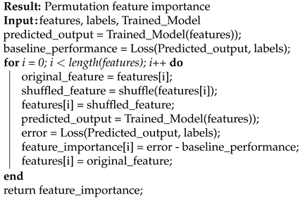
PI measures feature importance by calculating the changes in a model’s error when a feature is replaced by a shuffled version of itself. The algorithm of how PI quantifies feature importance is shown in Algorithm 1.

Algorithm 1: Algorithms of permutation importance.

The $shuffle$ function randomly changes the position of the row of the feature in every instance of the data. The magnitude of difference between $baseline\_performance$ and $error$ in Algorithm 1 signifies the importance of a feature. A feature has high importance if the performance of ML deviates significantly from the baseline after a shuffling; it therefore, has low importance if the performance does not change significantly. PI can be run on training or test data, but the test data are usually chosen to avoid retraining ML models to save computational overhead. If the computational cost is not an important factor to be considered, a drop-feature importance approach can be adopted to achieve greater accuracy. This is because, in PI, there is a possibility where a shuffled feature does not differ much from an unshuffled feature for some instances. For example, if a dataset has five instances and the original values for a feature is $[1,1,3,4,2]$, after shuffling, the new order of the feature is $[1,1,4,3,2]$; there is not much difference between the pre-shuffled and shuffled feature, making it difficult to determine its true importance accurately. In contrast, drop-feature importance excludes a feature, as opposed to performing its permutation, leading to more accurate quantification of importance. However, as it requires the ML model to be retrained every time a different feature is dropped, it is computationally expensive for high dimensional data. In this paper, we use PI over drop-feature importance to reduce the computational cost.

Additionally, we choose to use PI over MDI using Gini Importance. MDI tends to disproportionately increase the importance of continuous or high-cardinality categorical variables [23], leading to bias and unreliable feature importance measurements. PI is a model-agnostic approach to feature importance, and it can be used on GBT, RF, and DNN.

3.2. Shapley Additive Explanations

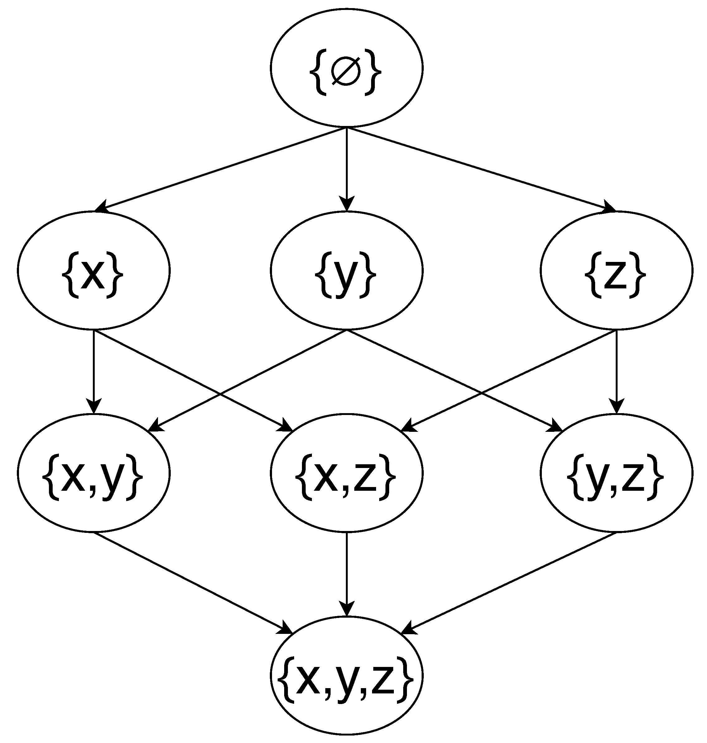
Other widespread feature importance model-agnostic approaches in addition to PI and MDA is SHAP. SHAP is a ML interpretability method that uses Shapley values, a concept originally introduced by Lloyd Shapley [39] in game theory to solve the problem of establishing each player contribution in cooperative games. Essentially, given a certain game scenario, the Shapley value is the average expected marginal contribution (MC) of a player after all possible combinations have been considered. For ML, SHAP determines the contribution of the available features of the model by assessing their every possible combination and by quantifying their importance. The total possible combinations can be represented through a power set. For example, in the case of three features, $PowerSet\{x,y,z\}$ the power set is $\left\{\right\{Ø\},\{x\},\{y\},\{z\},\{x,y\},\{x,z\},\{y,z\},\{x,y,z\left\}\right\}$. Furthermore, Figure 1 illustrates the relationships between the elements in the power set.

SHAP trains a ML model for each of the vertices shown in Figure 1. Therefore, there are $2^{\mathrm{number}\mathrm{of}\mathrm{features}}=2^3=8$ models trained to estimate the contribution of each feature. The number of models needed to estimate feature importance using SHAP increases exponentially with the number of features. However, there are tools, such as the Python library SHAP [40] to accelerate the process through approximations and sampling. The MC of a feature can be calculated by traversing the graph in Figure 1 and by summing up the changes in output where the feature is previously absent from the combinations. For example, to calculate the contribution of feature $\left\{x\right\}$, we can calculate the weighted average of the change in the output from $\{Ø\}$ to $\left\{x\right\}$, $\left\{y\right\}$ to $\{x,y\}$, $\left\{z\right\}$ to $\{x,z\}$, and $\{y,z\}$ to $\{x,y,z\}$. The MC of a feature x from $\{Ø\}$ to $\left\{x\right\}$ is as follows:

$$M{C}_{x,(Ø,x)}\left(i_0\right)=Outpu{t}_x\left(i_0\right)-{Output}_{Ø}\left(i_0\right)$$

(1)

where the $Output$ is the output of a ML model, and following Equation (1), we calculate the SHAP value of feature x of an instance $i_0$, as follows:

$$\begin{array}{cc}\hfill SHA{P}_x\left(i_0\right)=& w_1\ast M{C}_{x,(Ø,x)}\left(i_0\right)+\hfill \\ \hfill & w_2\ast M{C}_{x,(x,y)}\left(i_0\right)+\hfill \\ \hfill & w_3\ast M{C}_{x,(x,z)}\left(i_0\right)+\hfill \\ \hfill & w_4\ast M{C}_{x,(x,y,z)}\left(i_0\right)+\hfill \end{array}$$

(2)

The process is repeated for each feature to obtain the feature importance. The weights ($w_1,w_2,w_3$, and $w_4$) in Equation (2) sum to 1. The weights are calculated by taking the reciprocals of the number of possible combinations of MC for each row in Figure 1. For example, the weight of $w_1$ is ${\left(\genfrac{}{}{0pt}{}{3}{1}\right)}^{-1}$. To calculate the global importance of a feature, the absolute SHAP values are averaged across all instances.

Another approach is the model-agnostic feature importance method called local interpretable model-agnostic explanations (LIME) [41]. We did not choose LIME as a model interpretation method because it does not have a good global approximation of feature importance and it is only able to provide feature importance for individual instances. Furthermore, LIME is sensitive to small perturbations in the input, leading to different feature importance for similar input data [42].

3.3. Integrated Gradients

IG is a gradient-based method for feature importance. It determines the feature importance A in deep learning models by calculating the change in output, $f\left(x\right)$ relative to the change in input x. Additionally, the change in input features is approximated using an information-less baseline, b. The baseline input is a vector of zero in the case of regression to ensure that the baseline prediction is neutral and functions as a counterfactual. The features importance is denoted by the difference between the characteristics of the deep learning model’s output when features and baseline are used. The formula for feature importance using a baseline is as follows:

$$A_i^f(x,b)=f\left(x_i\right)-f\left(x[x_i=b_i]\right)$$

(3)

The individual feature is denoted by the subscript i. Equation (3) can be also written in the form of gradient-based importance as follows:

$$G_i^f(x,b)=(x_i-b_i)\frac{\partial f\left(x\right)}{\partial x_i}$$

(4)

IG obtains feature importance values by accumulating gradients of the features interpolated between the baseline value and the input. To interpolate between the baseline and the input, a constant, $\alpha$, with the value ranging from zero to one is used as follows:

$$I{G}_i^f(x,b)=(x_i-b_i){\int }_{\alpha =0}^1\frac{\partial f(b+\alpha (x-b\left)\right)}{\partial x_i}d\alpha$$

(5)

Equation (5) is the final form of IG used to calculate feature importance in a deep learning model.

4. Methodology

This section introduces our proposed MME Framework, where we employ multiple ML models and feature importance methods. We also introduce the different ensemble strategies investigated, including median, mode, box-whiskers, Modified Thompson Tau test, and majority vote. We also present the rank correlation with majority vote (RATE) fusion as a new ensembling strategy. Furthermore, this section also introduces our experimental design, including the benchmark datasets and how their generation is modulated. Subsequently, we discuss the data pre-processing, ML models employed, the evaluation metrics used, and the experiments conducted.

4.1. The Proposed Feature Importance Fusion Framework

4.1.1. Ensemble Feature Importance

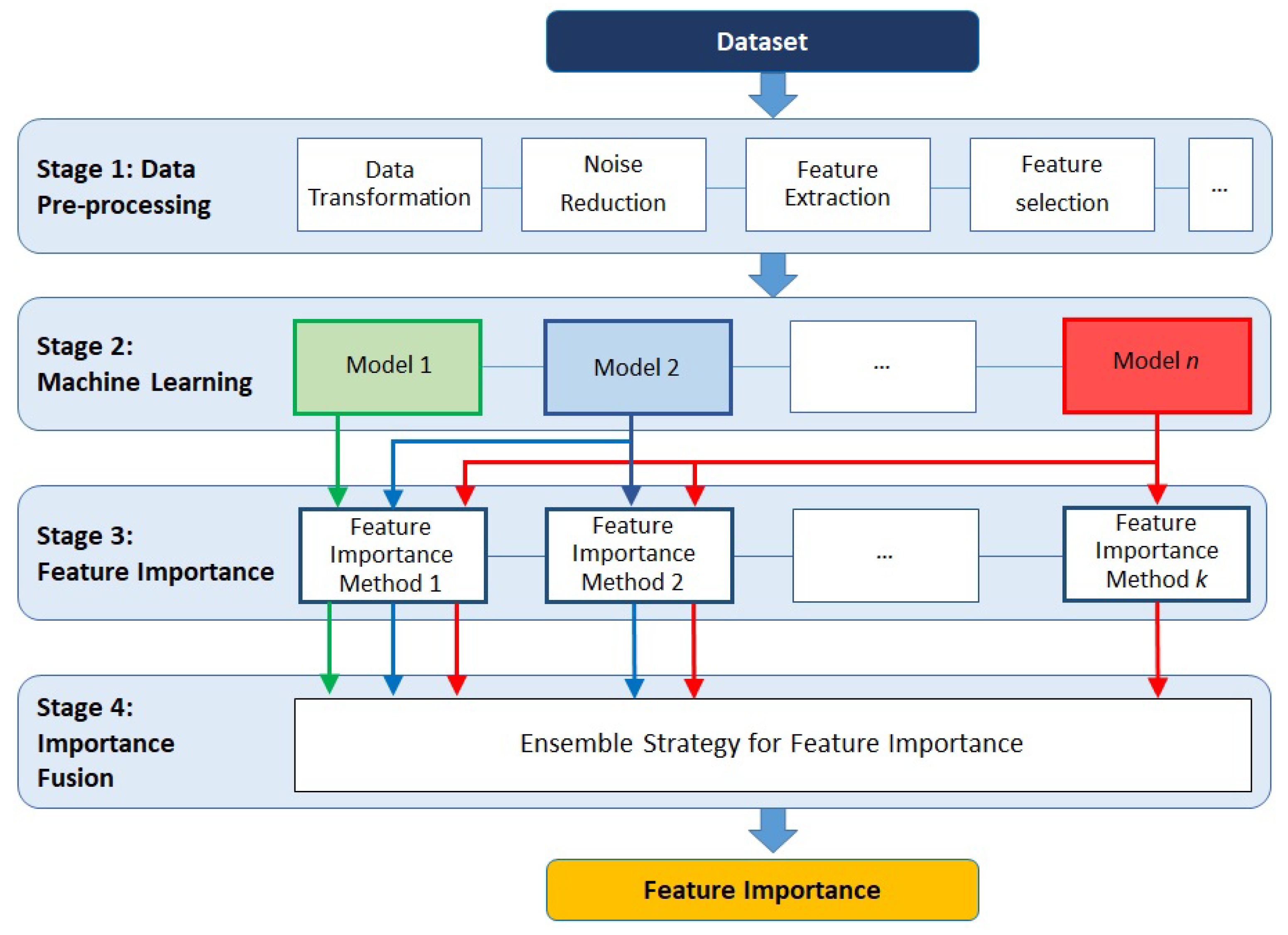
Figure 2 shows our MME Framework. On Stage 1, data undergo pre-processing, such as transformation, noise reduction, feature extraction and feature selection. This stage is required for our framework, as we need to ensure that the data have no inconsistencies and that the features used to train the machine learning models are orthogonal by removing noise and features that are collinear, which could negatively impact the model’s performance. The preference for features with low correlation guarantees that the feature importance calculation does not attribute random values of importance because a set of features contains similar information. No pre-processing is performed for this paper since the data are artificially created and undesirable features such as noise or non-informative features are kept to study the properties of the feature importance ensemble. On Stage 2, ML models are applied to the pre-processed data; subsequently, model-agnostics feature importance methods are applied to the ML models (Stage 3). The feature importance results are fused into a final feature importance in Stage 4.

In Stage 3 and Stage 4, when multiple methods and ML models are employed in ensemble feature importance, we obtain several vectors, Q, of feature importance values, A, as follows: $Q=[A_1,A_2,...,Ai]$, where i is the number of features and there is one Q for each ML model and feature importance technique combination. We need to establish a final decision from those vectors. Therefore, first we reduce the noise and anomalies in the decision. The feature importance vectors can be denoted as follows: $\overline{\overrightarrow{V}}=[Q_1,Q_2,...,Q_N]$, where N is the sum of each model multiplied by the number of feature importance methods used. To reduce the noise and variance, we can take the average of all feature importance vectors, $\overline{\overrightarrow{V}}$, which produces the variance, ${\sigma }^2/N$. As N increases, the variance decreases. The variance and correctness of final feature importance vector can be further improved if the anomalies are removed prior to taking the average.

4.1.2. Ensemble Strategies

Within our MME Framework, the importance calculated is stored in a matrix, $\overline{\overrightarrow{V}}$, and the ensemble strategy, which can be obtained in several ways, is used to determine the final feature importance values from $\overline{\overrightarrow{V}}$. The most common ensemble strategy, as discussed in Section 2, is to use the average values. However, this is not the most suitable ensemble strategy in cases where one or more of the feature importance approaches produce outliers compared with the majority of responses. Therefore, in addition to the mean, we also investigate data fusion using median, mode, box-whiskers, majority vote, Modified Thompson Tau test, and our novel fusion approach RATE. The mode of a continuous probability distribution is any value at which its probability density function has a locally maximum value. By employing box-whisker plots, the anomalous feature importance is identified and excluded from the ensemble if its value is outside of 1.5 times the interquartile range (IQR). IQR is the difference between the third and first quartiles of the feature importance values. For majority vote, each vector in the feature importance matrix has their features ranked based on their importance. Subsequently, the final feature importance is the average of the most common rank order for each feature. For example, feature $X_i$ has a final rank vector of $[1,1,1,2]$, where each rank $r_k$ is established by a different feature importance method k. The final feature importance value for feature $X_i$ is the average value from the three feature importance methods that ranked it as one. Modified Thompson Tau test is a statistical anomaly detection method using t-test to eliminate values that are above two standard deviations.

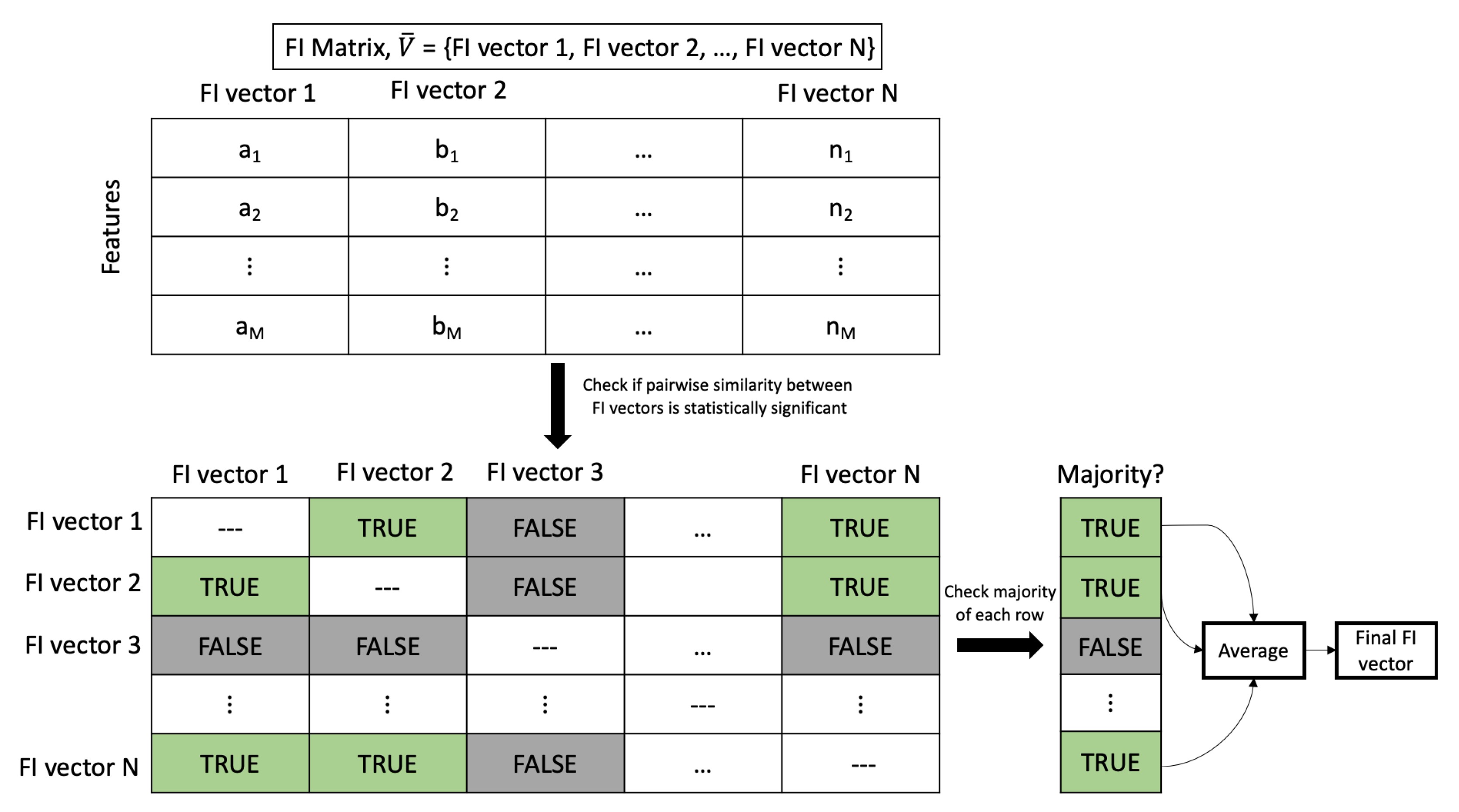
RATE is our novel fusion approach that combines the statistical test feature rank, with majority vote. Rank correlation is the calculation of the statistical dependence between two rank variables. In this case, the rank variables are the ranking of feature importance by each combination of ML model and feature importance method pair. RATE combines the advantage of using a statistical approach to rank feature importance and anomaly removal with majority vote. The steps used in RATE are illustrated in Figure 3. The input to RATE is the feature importance matrix, $\overline{\overrightarrow{V}}$. $\overline{\overrightarrow{V}}$ is the matrix that has the individual feature importance from different models, and it has the shape of $N\ast M$, where N is the feature importance vectors from different importance calculation methods and M is the number of features. We calculate the pairwise rank correlation between each feature importance vectors in the matrix $\overline{\overrightarrow{V}}$ to obtain the rank and the general correlation coefficient values [43]. Using the rank and correlation value, we determine whether the correlation between the vectors is statistically significant (p-value less than 0.05). The p-values are stored in a separate matrix that is converted to a truth table. If the pairwise p-value is less than 0.05, it is given a value of ‘TRUE’; otherwise, it is ‘FALSE’. Using the truth table along with majority vote, we determine which feature importance vector overall does not correlate with the majority of vectors and should be discarded. The remaining feature importance vectors are averaged as the final feature importance.

4.2. Data Generation

The data investigated are generated using Python’s Scikit-learn library [44] and more specifically the $make\_regression$ function with different characteristics to mimic a variety of real-world regression scenarios. The features generated are random but well conditioned, centered, and Gaussian with unit variance by default. The correlation between features is also random. The parameters used to modulate the creation of the datasets are the standard deviations of the Gaussian distributed noise applied to the data, the number of features included, and the percentage of informative features. Their values are shown in

Table 1. Parameters to generate the datasets used to test our MME Framework.

Parameters	Description	Parameters’ Value
Noise	Standard deviation of Gaussian noise applied to the output.	0, 2, 4
Informative level (%)	Percentage of informative features. Non-informative features do not contribute to the output.	20, 40, 60, 80, 100
Number of features	Total number of features used to generate output values.	20, 60, 100

. We add Gaussian-distributed noise with different standard deviations to the output as it has a more significant effect on prediction accuracy than that in the features [45]. Although noise increases the ML models’ estimated error [45,46], studies investigating the relationship between data noise and feature importance error are scarce. Similarly, the impact of the number of features and how many features within the set are relevant to importance error is unknown. Furthermore, informative levels of features are included. In real-world data, not all features are employed by the learned models to perform regression or classification tasks. A combination of values from each parameter in the table forms a dataset, and permutations of those parameters form a total of 45 datasets. For each dataset, we conduct ten experimental runs to ensure that the results are stable and reliable.

The data pre-processing in our case consists of scaling the input data to the range between zero and one. Scaling the data accelerates the learning process and reduces model error for neural networks [47]. Additionally, it allows for equal weighting of all features and therefore reduces bias during learning. Other common pre-processing steps such as anomaly removal and normalisation are not included as the data creation process is controlled.

4.3. Machine Learning Models

The ML approaches employed in our experiments are RF, GBT, SVM, and DNN; the hyperparameters adopted are shown in

Table 2. Hyperparameter values for Random Forest, Gradient Boosted Trees, Support Vector Regression, and Deep Neural Network for all experiments.

Models	Hyperparameters	Values
Random Forest	Number of trees	700
	Maximum depth of trees	7 levels
	Minimum samples before split	2
	Maximum features	$\sqrt{p}$
	Bootstrap	True
Gradient Boosted Trees	Number of trees	700
	Learning rate	0.1
	Maximum depth of trees	7 levels
	Loss function	Least square
	Maximum features	$\sqrt{p}$
	Splitting criterion	Friedman MSE
Support Vector Regressor	Kernel	Linear
	Regularisation parameter	2048
	Gamma	1 × 10${}^{-7}$
	Epsilon	0.5
Deep Neural Network	Number of layers	8
	Number of nodes for each layer	64, 64, 32, 16, 8, 6, 4, 1
	Activation function for each layer	ReLU, except for output is linear
	Loss function	MSE
	Optimiser	Rectified Adam with LookAhead
	Learning rate	0.001
	Kernel regulariser	L2 (0.001)
	Dropout	0.2

. We optimise the models using random hyperparameter search [48], using conditions at the upper and lower limits of the parameters used for the datasets generation. The models are not optimised for individual datasets. We keep the model’s hyperparameters constant as it might be a factor that affects feature importance accuracy. We therefore limit our objectives to investigating how data characteristics affect interpretability methods and how the appropriate fusion of different feature importance methods produces less biased estimates. Furthermore, we try to minimise overfitting in the deep learning model by adopting dropout [49] and L2 kernel regularisation [50]. The number of epochs for the training of deep learning model is not fixed as early stopping is used. If the loss remains constant for 10 epochs, the training is automatically stopped.

The feature importance methods employed by each ML models are listed in

Table 3. Interpretability methods employed by each ML model for feature importance fusion.

Models	Interpretability Methods
Random Forest	Permutation Importance, SHAP
Gradient Boosted Trees	Permutation Importance, SHAP
Support Vector Regressor	Permutation Importance, SHAP
Deep Neural Network	Permutation Importance, SHAP, and Integrated Gradient

. For SHAP, we employ weighted k-means to summarise the data before estimating the values of SHAP. Each cluster is weighted by the number of points they represent. Using k-means to summarise the data has the advantage of lowering computational cost but slightly decreasing the accuracy of SHAP values. However, we compare the SHAP values from data with and without k-means for several datasets and found the SHAP values to be almost identical.

We train and evaluate the ML models using Intel(R) Xeon(R) CPU @ 2.20 GHz and the deep learning model is trained on Dell 16GB NVIDIA Tesla T4.

4.4. Evaluation Metrics

To evaluate the performance of the ensemble feature importance and the different ensemble strategies, we employ three different evaluation metrics, namely, Mean Absolute Error (MAE), Root Mean Square Error (RMSE), and $R^2$.

5. Results and Discussion

5.1. Single-Method Ensemble vs. Our Multi-Method Ensemble Framework

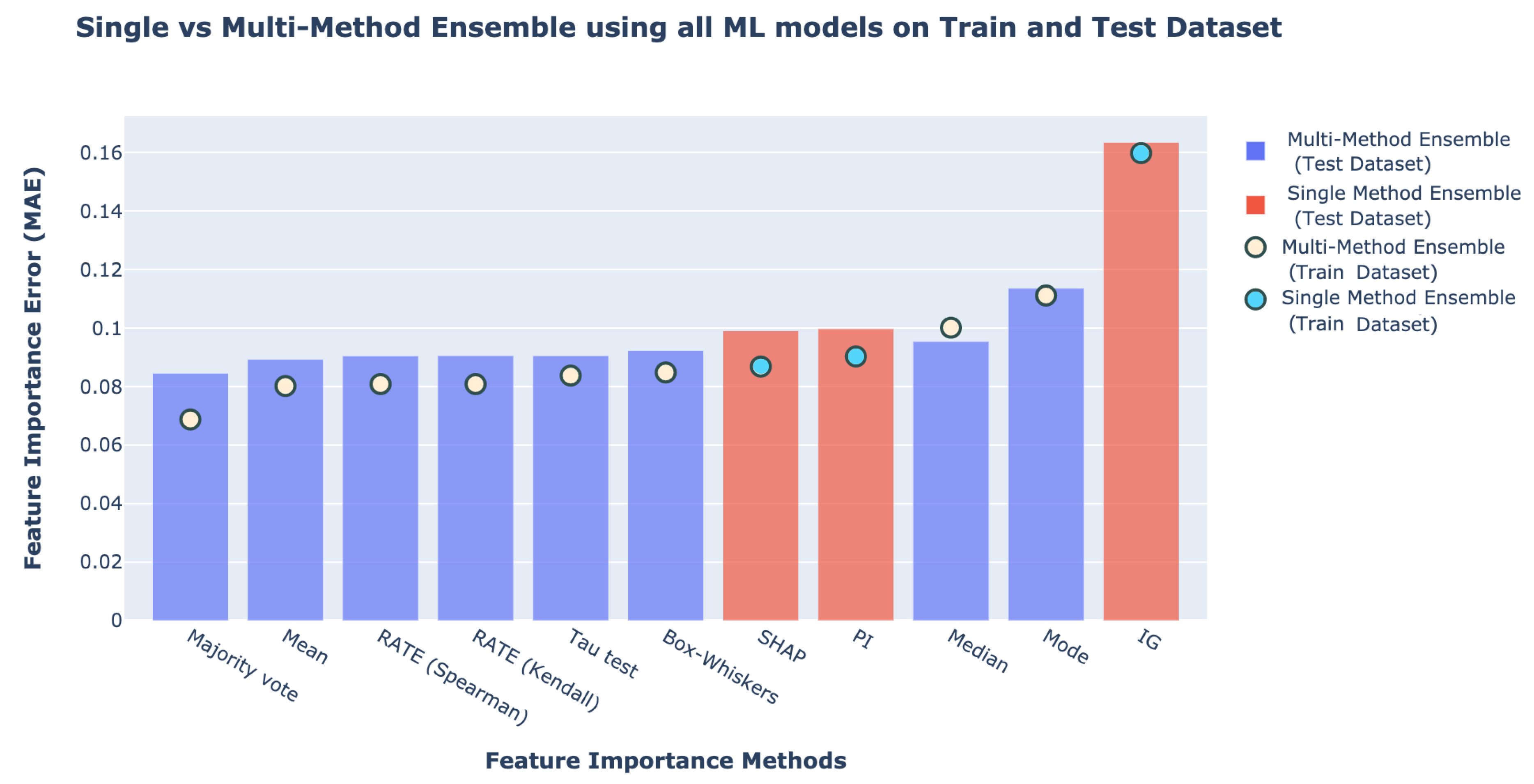
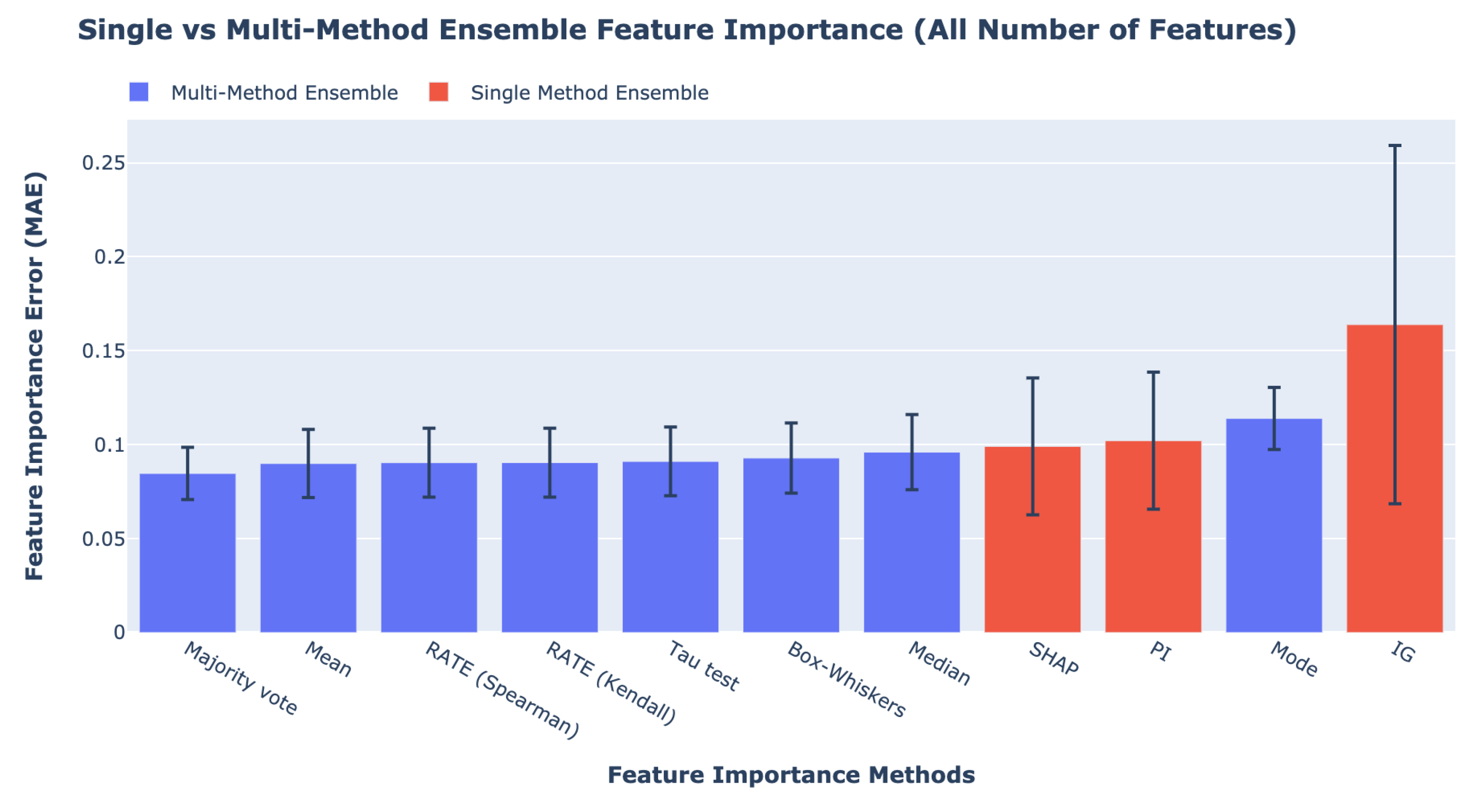
In order to compare the results of SME and our MME Framework, Figure 4 shows the average MAE of all SME and the multiple fusion implementations of our MME Framework across all datasets. Comparison of the average results between SME and our MME Framework in the RMSE, and the $R^2$ metrics are shown in Sections S1.1 and S1.2 of the Supplementary Materials. The ensemble method with the least feature importance error is our MME Framework using majority vote for fusion, followed by the MME Framework with mean and RATE. SME such as SHAP, PI, and IG produce the worst results. The circles and bars in the figure represent the feature importance errors on the training and test datasets, respectively. The feature importance errors on the training dataset are slightly lower than the errors on the test dataset.

5.2. Effect of Noise Level, Informative Level, and Number of Features on All Feature Importance

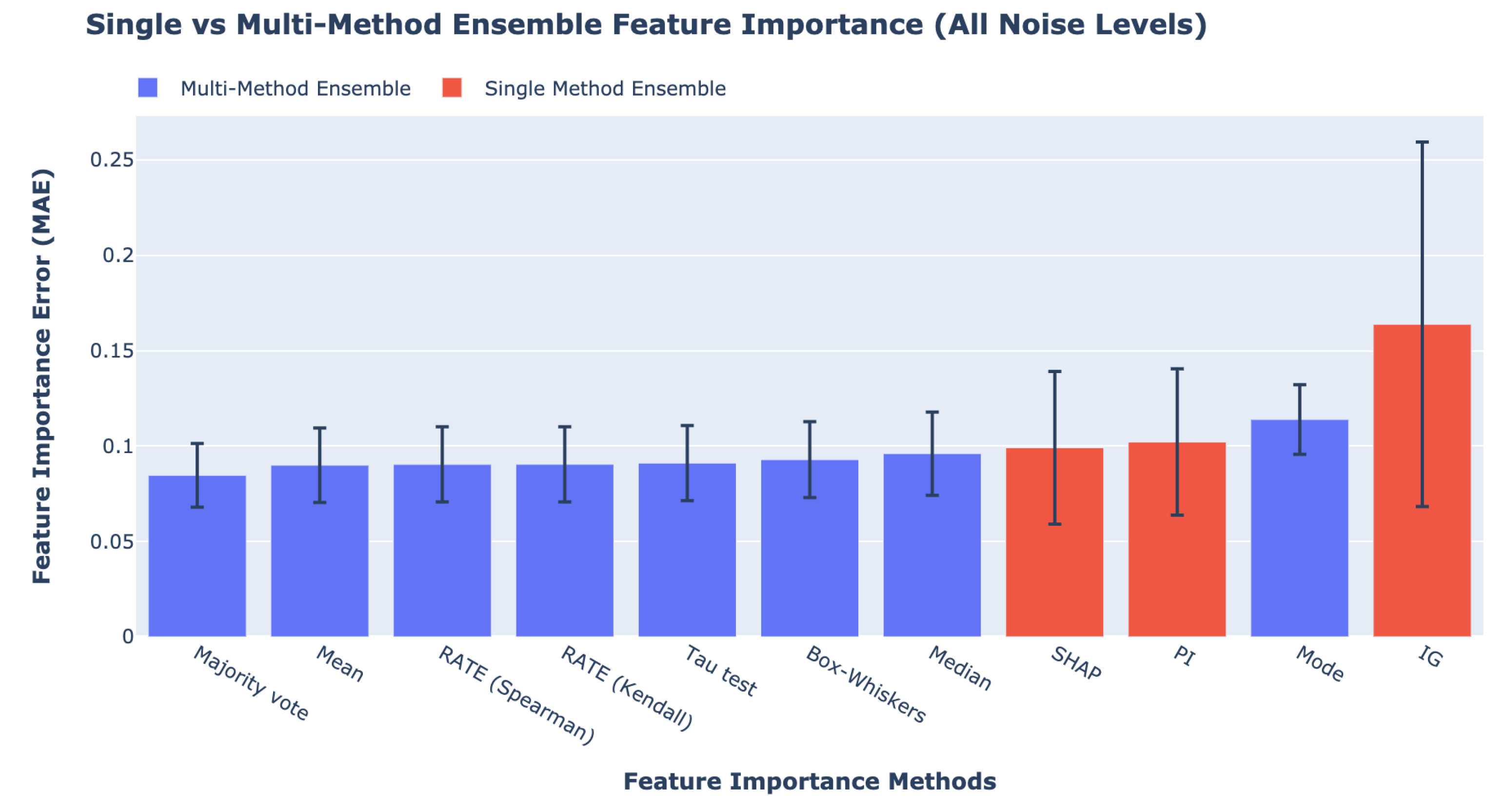
Figure 5 shows the feature importance results of SME and the MME Framework with different fusion strategies averaged across three different noise levels in the data. The results on the effect of noise in data on ensemble feature importance using the RMSE and $R^2$ metrics are shown in Sections S1.3 and S1.4 of the Supplementary Material. The best performing ensemble method averaged across all noise levels is MME Framework using majority vote. The MME Framework that uses majority vote outperforms the best SME method, SHAP, by 14.2%. In addition,

Table 4. Summary of feature importance MAE between different methods using SME and the MME Framework for different noise levels.

	Models	Noise Level (Standard Deviation)
		0 (${10}^{-2}$)	2 (${10}^{-2}$)	4 (${10}^{-2}$)
SME	PI	10.1 ± 2.0	9.8 ± 1.9	10.7 ± 2.6
	SHAP	9.8 ± 2.2	9.7 ± 2.2	10.0 ± 2.3
	IG	15.8 ± 9.5	16.7 ± 9.5	16.5 ± 9.5
MME	RATE (Kendall)	8.8 ± 3.2	8.8 ± 3.2	9.4 ± 3.6
	RATE (Spearman)	8.8 ± 3.2	8.8 ± 3.2	9.4 ± 3.6
	Median	9.5 ± 3.7	9.0 ± 3.4	10.1 ± 4.0
	Mean	8.8 ± 3.2	8.7 ± 3.2	9.4 ± 3.6
	Mode	12.2 ± 3.4	10.7 ± 3.0	11.1 ± 3.0
	Box-whiskers	9.1 ± 3.3	9.1 ± 3.3	9.5 ± 3.6
	Tau test	8.9 ± 3.3	8.8 ± 3.2	9.5 ± 3.6
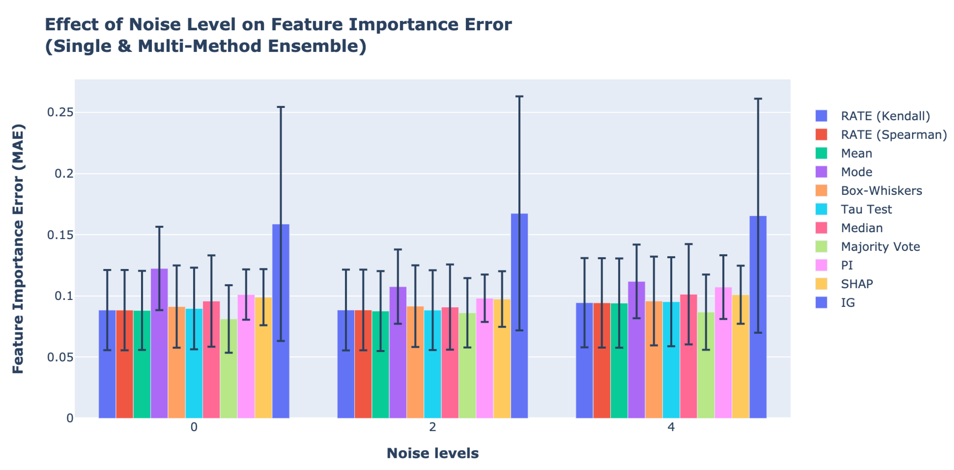
	Majority vote	8.1 ± 2.7	8.6 ± 2.8	8.6 ± 3.0

and Figure 6 show how the feature importance errors change for all SME and MME Framework methods as the noise level increases. In Table 4, we observe that the MAE decreases marginally, from a noise level of 0 standard deviations to 2 standard deviations, and then, it increases again by four times the standard deviation. The addition of 2 standard deviation noise to the dataset improves the generalisation performance of ML models, leading to lower errors [51]. However, the feature importance errors increase when the noise in the dataset reaches four times the standard deviation, indicating that the noise level has negatively impacted ML model performance. Overall, however, the noise levels have little effect on the feature importance errors. The results also reveal that the MME Framework with majority vote achieves the best feature importance estimates for our data.

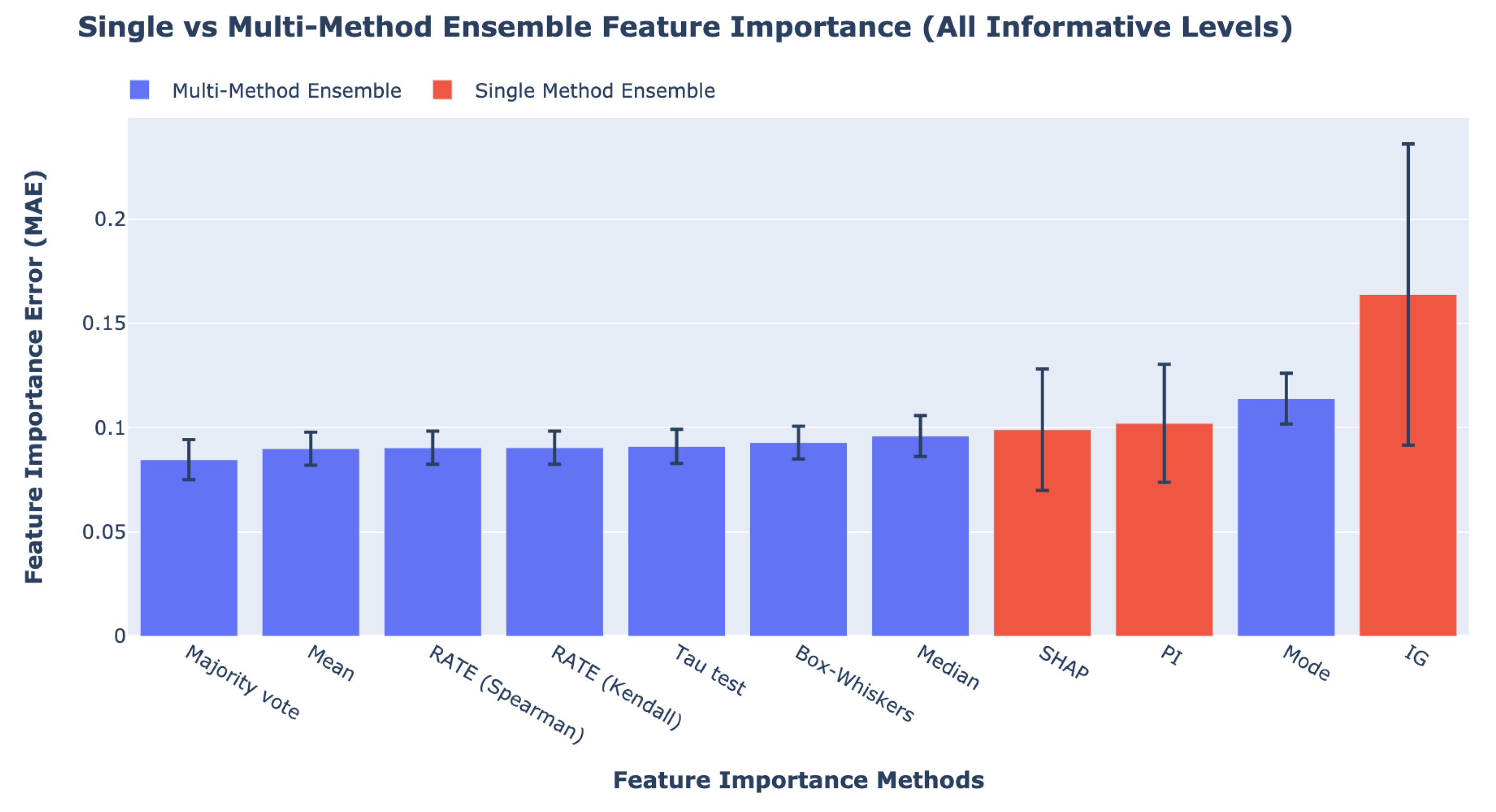
Figure 7 presents the feature importance MAE error for all SME and the MME Framework with different fusion strategies averaged across five different feature informative levels in the data. The results on the effect of feature informative levels on ensemble feature importance using the RMSE and $R^2$ metrics are shown in Sections S1.5 and S1.6 of the Supplementary Material. The best performing method is MME with majority vote followed by MME with mean and RATE. All MME Framework methods except for that with the mode outperform SME by more accurately quantifying the feature importance. The error bar (standard deviation) for the effect of feature informative levels in Figure 7 has a smaller range than the effect of noise and the effect of number of features. The low standard deviation indicates that the feature informative levels explain most of the variances. From

Table 5. Summary of feature importance MAE between different SME and our the MME Framework for different percentages of informative level.

	Models	Feature Informative Level (%)
		20 (${10}^{-2}$)	40 (${10}^{-2}$)	60 (${10}^{-2}$)	80 (${10}^{-2}$)	100 (${10}^{-2}$)
SME	PI	2.7 ± 0.4	6.7 ± 0.8	11.2 ± 2.0	13.8 ± 1.0	16.5 ± 1.3
	SHAP	2.2 ± 0.4	5.8 ± 0.8	9.7 ± 1.0	14.2 ± 1.5	17.3 ± 1.9
	IG	6.3 ± 7.2	10.7 ± 7.2	15.8 ± 7.2	22.2 ± 7.2	26.7 ± 7.2
MME	RATE (Kendall)	2.1 ± 0.4	5.4 ± 1.1	9.3 ± 1.5	12.3 ± 1.6	15.9 ± 3.0
	RATE (Spearman)	2.1 ± 0.5	5.4 ± 1.1	9.3 ± 1.5	12.3 ± 1.6	15.9 ± 3.0
	Median	2.0 ± 0.6	5.9 ± 1.4	10.2 ± 1.8	13.0 ± 2.4	16.7 ± 3.5
	Mean	2.1 ± 0.5	5.4 ± 1.1	9.4 ± 1.5	12.3 ± 1.6	15.7 ± 3.0
	Mode	7.0 ± 2.0	9.0 ± 3.1	12.4 ± 3.1	13.3 ± 1.9	15.0 ± 3.0
	Box-whiskers	2.1 ± 0.6	5.6 ± 1.1	9.5 ± 1.4	12.9 ± 1.7	16.1 ± 2.9
	Tau test	2.0 ± 0.6	5.6 ± 1.2	9.5 ± 1.5	12.4 ± 1.7	15.7 ± 3.0
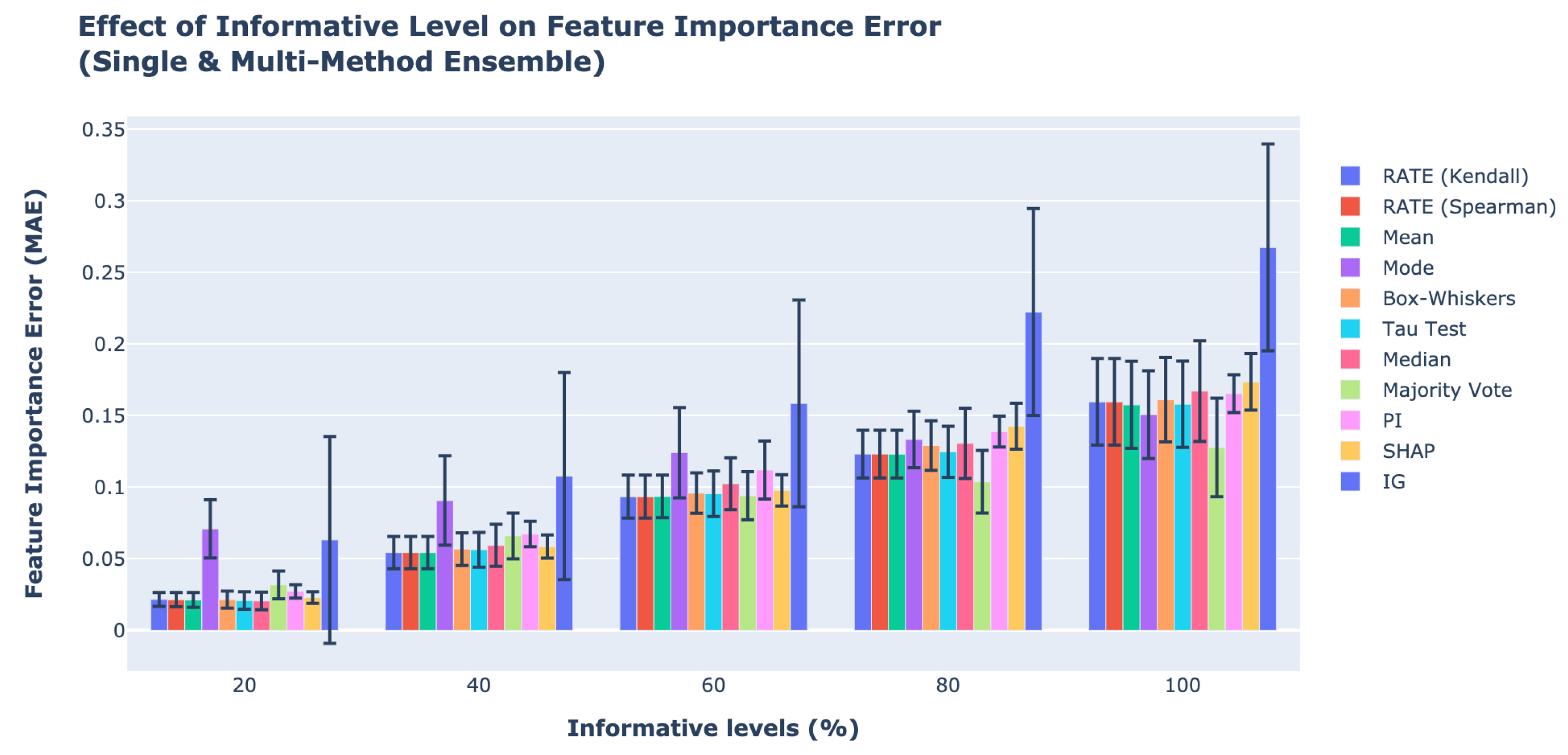
	Majority vote	3.1 ± 0.9	6.5 ± 1.5	9.4 ± 1.6	10.3 ± 2.1	12.7 ± 3.4

, we observe that, when 20% of the features are informative, the best feature importance methods are MME Framework with Modified Thompson tau test and median, and they outperform the best SME method, SHAP, by 9.1%. For the 40% feature informative level, the MME Framework with RATE (Kendall and Spearman) and mean have the lowest errors, with 6.9% improvement over SME with SHAP. For the 60% feature informative level, the MME Framework using RATE (Kendall and Spearman) have the best results, with a 4.1% improvement over SME with SHAP. Furthermore, the MME Framework with majority vote obtains the lowest error for both 80% and 100% feature informative level. The best performing SME is using PI. MME with majority votes outperforms SME’s best results by 25.4% and 23.0% for 80% and 100% feature informative level, respectively.

Figure 8 shows the relationship between the MAE of feature importance errors and the percentage of feature informative level. As the percentage of feature informative level increases the feature importance errors increases. The higher number of contributing (non-zero) features to the output increases the difficulty of quantifying feature importance leading to higher errors.

Figure 9 depicts the average of all SME and the MME Framework with fusion methods across 20, 60, and 100 features. The results on the effect of number of features on ensemble feature importance using the RMSE and $R^2$ metrics are shown in Sections S1.7 and S1.8 of the Supplementary Material. Similar to the effect of noise level and the percentage of informative features on feature importance errors, the MME Framework with majority vote has the lowest error across all features. The error bar for the effect of feature number in Figure 9 has a smaller range compared with the feature importance errors of the effect of noise but larger than the effect of number of features. From

Table 6. Summary of feature importance MAE between different SME and our MME Framework for different number of features.

	Models	Number of Features
		20 (${10}^{-2}$)	60 (${10}^{-2}$)	100 (${10}^{-2}$)
90SME	PI	7.5 ± 1.8	10.8 ± 2.0	12.2 ± 2.4
	SHAP	6.1 ± 1.5	10.3 ± 2.2	13.1 ± 2.4
	IG	15.8 ± 9.5	16.1 ± 9.5	17.1 ± 9.5
MME	RATE (Kendall)	6.3 ± 2.3	9.4 ± 3.1	11.3 ± 3.8
	RATE (Spearman)	6.37 ± 2.3	9.4 ± 3.1	11.3 ± 3.8
	Median	6.0 ± 2.3	10.6 ± 3.8	12.0 ± 3.9
	Mean	6.2 ± 2.2	9.3 ± 3.1	11.3 ± 3.8
	Mode	14.8 ± 3.6	9.6 ± 2.3	9.7 ± 2.4
	Box-whiskers	6.5 ± 2.5	9.8 ± 3.2	11.4 ± 3.7
	Tau test	6.1 ± 2.4	9.7 ± 3.2	11.4 ± 3.7
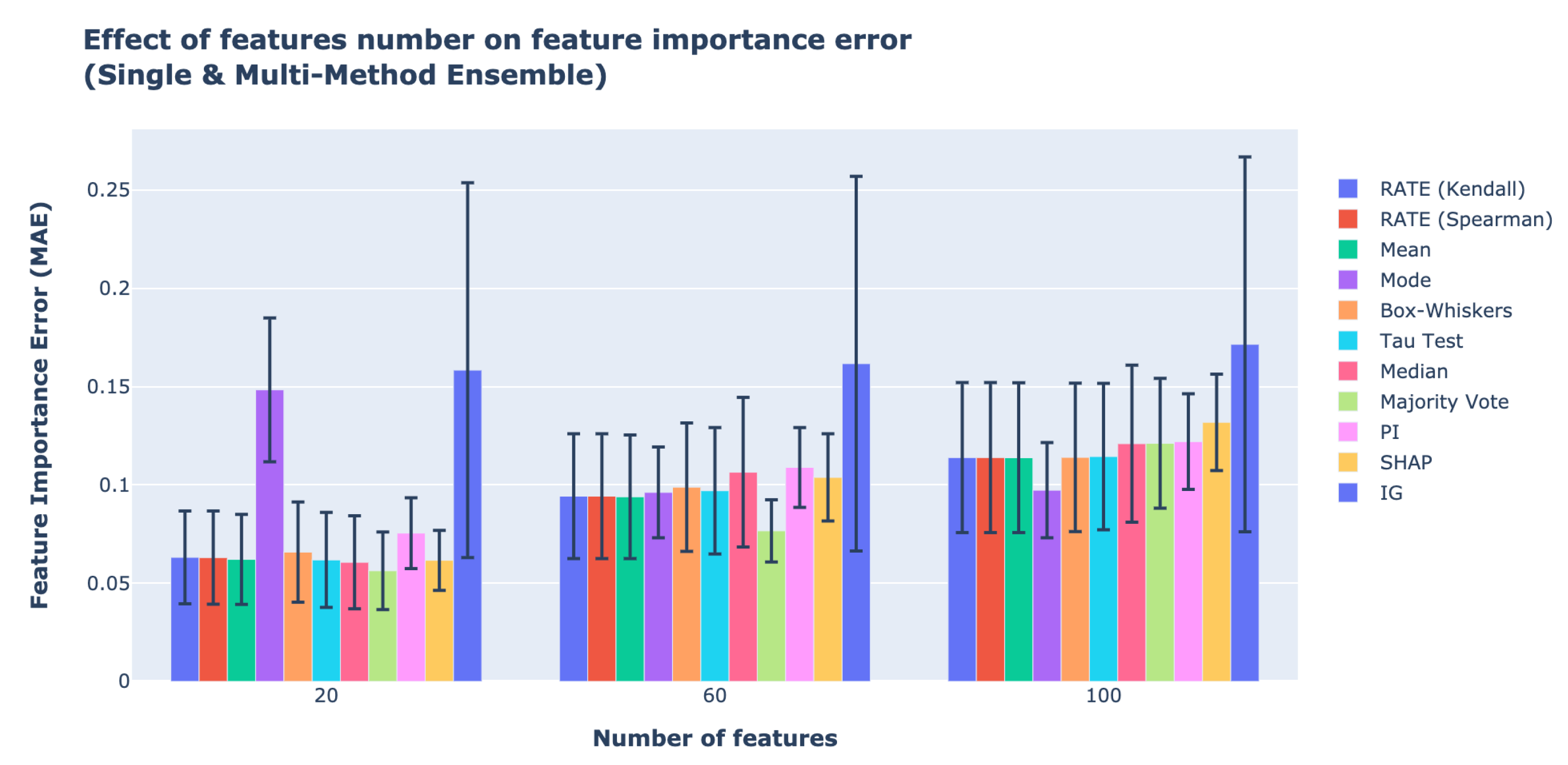
	Majority vote	5.6 ± 1.9	7.6 ± 1.5	12.1 ± 3.3

, we observe that, when there are 20 and 40 features, the method with the lowest feature importance errors is the MME Framework with majority vote, and it outperforms the best SME method—SHAP by 8.2% and 26.2%, respectively. For 100 features, the MME Framework using the mode is the most accurate method, and it outperforms the best SME method, PI by 20.5%. For SME, PI has lower feature importance errors compared with SHAP as the number of informative features and features increases.

Figure 10 shows the relationship between the MAE of feature importance and the number of features as they increase. The higher number of features increases the difficulty of quantifying feature importance accurately.

5.3. Discussion

Overall, the results show that our MME Framework outperforms SME for our case studies. In particular, the MME Framework with majority vote as an ensemble strategy for the three different combinations of factors—(i) noise level, (ii) feature informative level, and (iii) number of features—has achieved the best results. The robustness of our framework compared with SMEs becomes even more evident as the number of features and the number of informative features increases. The results also reveal that the noise in the data does not affect the final feature importance estimates, as there are no significant changes as the noise increases.

One advantage of using our model-agnostic MME Framework is that it avoids the worst-case scenario for feature importance estimates due to the inherent advantage of ensembles being more robust against spread and dispersion of the predictions. Additionally, using only one set of explainability can potentially bias the feature importance estimates. Similarly, the feature importance estimates might be biased if only a single method is employed as it might not consider the synergy between orthogonal features. By fusing feature importance estimates of multiple ML models and methods, we can achieve a final feature importance estimates that is more robust. For safety-critical systems, it is important for the feature importance estimates to be robust to noise, biases, and anomalies for end-users to explain the results of ML models accurately.

Conversely, this can also be a disadvantage as the best performing feature importance estimate might be moderated by worse methods. However, in real-world, safety-critical systems where the ground truth is unknown, it is important to rely on not only a single method but also the potential bias it might produce. In scenarios where all feature importance determined by different methods disagree or there is no consensus on feature importance, RATE or majority vote is reduced to the average of all feature importance vectors. Under such circumstances, the best option for safety is to further investigate the reasons for disagreement between ML model or feature importance techniques. Furthermore, while the majority vote achieves the best results for many different data characteristics in this paper, it is not always the case. Further studies are necessary to decide which ensemble method is definitely better for specific data characteristics.

For our experiments, we keep the hyperparameters of each ML model constant as their case-based optimisation is likely to affect feature importance estimates for different data characteristics. In the future, it is necessary to further investigate the interplay between parameter optimisation and feature importance. In addition, other factors such as covariate drift on the test dataset and imbalanced datasets should be included in the framework tests.

6. Conclusions and Future Work

In this paper, we presented a novel framework to perform feature importance fusion using an ensemble of different ML models and different feature importance methods called MME. Overall, our framework performed better than traditional single model-agnostic approaches, where only one feature importance method with multiple ML models is employed. Additionally, we compared different ensemble strategies for our MME Framework such as measurements of central tendency such as median, mean, and mode and anomaly detection methods such as box-whiskers, Modified Thompson Tau test, and majority vote. In addition, we introduced a new ensemble strategy named RATE that combined rank correlation and majority vote. Furthermore, we studied the efficacy of MME Framework and SME on a combination of three different factors: (i) noise level, (ii) percentage of informative features, and (iii) the number of features. We found that different noise levels had a minimal effect on feature importance, whereas the feature importance error increased with the percentage of informative features and number of features in data. For the case studies investigated, the MME Framework with majority vote is often the best performing method for all three data factors, followed by the MME Framework with RATE and mean. When the number of features and the number of informative features are low, the performance of MME Framework is only marginally better than SME.

We showed that the MME Framework avoids the worst-case scenario in predicting feature importance. Additionally, the MME Framework is able to increase the quality of feature importance estimates by making it more robust against noise, biases, and anomalies. Despite its advantages, there are several shortcomings in the proposed method and our experimental approach that can be improved in future work. One improvement would be to include more feature importance methods and ML models into the MME Framework to increase the number of methods to investigate their impact on variance and in overall consensus of importance. Another possibility is to integrate the feature importance ensemble into a neural network to internally induce bias in the neural networks to focus on relevant features to decrease training time and to improve accuracy. Finally, for the experimental aspect, several other factors could potentially affect the feature importance estimates, such as hyperparameter optimisations of ML models, imbalance of the datasets, the presence of anomalies in data, and the efficacy of the framework in complex real-world data should be investigated.

References

- Uddin, M.Z.; Hassan, M.M.; Alsanad, A.; Savaglio, C. A body sensor data fusion and deep recurrent neural network-based behavior recognition approach for robust healthcare. Inf. Fusion 2020, 55, 105–115. [Google Scholar] [CrossRef]
- Miotto, R.; Wang, F.; Wang, S.; Jiang, X.; Dudley, J.T. Deep learning for healthcare: Review, opportunities and challenges. Briefings Bioinform. 2018, 19, 1236–1246. [Google Scholar] [CrossRef] [PubMed]
- Cruz-Roa, A.; Gilmore, H.; Basavanhally, A.; Feldman, M.; Ganesan, S.; Shih, N.N.; Tomaszewski, J.; González, F.A.; Madabhushi, A. Accurate and reproducible invasive breast cancer detection in whole-slide images: A Deep Learning approach for quantifying tumor extent. Sci. Rep. 2017, 7, 46450. [Google Scholar] [CrossRef] [Green Version]
- Rengasamy, D.; Morvan, H.P.; Figueredo, G.P. Deep learning approaches to aircraft maintenance, repair and overhaul: A review. In Proceedings of the 2018 21st International Conference on Intelligent Transportation Systems (ITSC), Maui, HI, USA, 4–7 November 2018; pp. 150–156. [Google Scholar]
- Rengasamy, D.; Jafari, M.; Rothwell, B.; Chen, X.; Figueredo, G.P. Deep Learning With Dynamically Weighted Loss Function for Sensor-based Prognostics and Health Management. Sensors 2020, 20, 723. [Google Scholar] [CrossRef] [Green Version]
- Yang, T.; Chen, B.; Gao, Y.; Feng, J.; Zhang, H.; Wang, X. Data mining-based fault detection and prediction methods for in-orbit satellite. In Proceedings of the 2013 2nd International Conference on Measurement, Information and Control, Harbin, China, 16–18 August 2013; Volume 2, pp. 805–808. [Google Scholar]
- Mafeni Mase, J.; Chapman, P.; Figueredo, G.; Torres Torres, M. Benchmarking Deep Learning Models for Driver Distraction Detection. In Machine Learning, Optimization, and Data Science (LOD) 2020; Springer: Cham, Switzerland, 2020. [Google Scholar]
- Eraqi, H.; Abouelnaga, Y.; Saad, M.; Moustafa, M. Driver Distraction Identification with an Ensemble of Convolutional Neural Networks. J. Adv. Transp. 2019, 2019, 4125865. [Google Scholar] [CrossRef]
- Mafeni Mase, J.; Agrawal, U.; Pekaslan, D.; Torres Torres, M.; Figueredo, G.; Chapman, P.; Mesgarpour, M. Capturing Uncertainty in Heavy Goods Vehicle Driving Behaviour. In Proceedings of the IEEE International Conference on Intelligent Transportation Systems, Rhodes, Greece, 20–23 September 2020. [Google Scholar]
- Farrar, C.R.; Worden, K. Structural Health Monitoring: A Machine Learning Perspective; John Wiley & Sons: Hoboken, NJ, USA, 2012. [Google Scholar]
- Catbas, F.N.; Malekzadeh, M. A machine learning-based algorithm for processing massive data collected from the mechanical components of movable bridges. Autom. Constr. 2016, 72, 269–278. [Google Scholar] [CrossRef] [Green Version]
- Zhang, B.; Liu, S.; Shin, Y.C. In-Process monitoring of porosity during laser additive manufacturing process. Addit. Manuf. 2019, 28, 497–505. [Google Scholar] [CrossRef]
- Wang, J.; Ma, Y.; Zhang, L.; Gao, R.X.; Wu, D. Deep learning for smart manufacturing: Methods and applications. J. Manuf. Syst. 2018, 48, 144–156. [Google Scholar] [CrossRef]
- Seshia, S.A.; Sadigh, D.; Sastry, S.S. Towards verified artificial intelligence. arXiv 2016, arXiv:1606.08514. [Google Scholar]
- Brundage, M.; Avin, S.; Wang, J.; Belfield, H.; Krueger, G.; Hadfield, G.; Khlaaf, H.; Yang, J.; Toner, H.; Fong, R.; et al. Toward trustworthy AI development: Mechanisms for supporting verifiable claims. arXiv 2020, arXiv:2004.07213. [Google Scholar]
- Pham, M.; Goering, S.; Sample, M.; Huggins, J.E.; Klein, E. Asilomar survey: Researcher perspectives on ethical principles and guidelines for BCI research. Brain-Comput. Interfaces 2018, 5, 97–111. [Google Scholar] [CrossRef]
- Rudin, C. Stop explaining black box machine learning models for high stakes decisions and use interpretable models instead. Nat. Mach. Intell. 2019, 1, 206–215. [Google Scholar] [CrossRef] [Green Version]
- Adadi, A.; Berrada, M. Peeking inside the black-box: A survey on Explainable Artificial Intelligence (XAI). IEEE Access 2018, 6, 52138–52160. [Google Scholar] [CrossRef]
- Gunning, D. Explainable Artificial Intelligence (XAI); DARPA: Arlington County, VA, USA, 2017; Volume 2. [Google Scholar]
- Arrieta, A.B.; Díaz-Rodríguez, N.; Del Ser, J.; Bennetot, A.; Tabik, S.; Barbado, A.; García, S.; Gil-López, S.; Molina, D.; Benjamins, R.; et al. Explainable Artificial Intelligence (XAI): Concepts, taxonomies, opportunities and challenges toward responsible AI. Inf. Fusion 2020, 58, 82–115. [Google Scholar] [CrossRef] [Green Version]
- Chakraborty, S.; Tomsett, R.; Raghavendra, R.; Harborne, D.; Alzantot, M.; Cerutti, F.; Srivastava, M.; Preece, A.; Julier, S.; Rao, R.M.; et al. Interpretability of deep learning models: A survey of results. In Proceedings of the 2017 IEEE SmartWorld, Ubiquitous Intelligence & Computing, Advanced & Trusted Computed, Scalable Computing & Communications, Cloud & Big Data Computing, Internet of People and Smart City Innovation (SmartWorld/SCALCOM/UIC/ATC/CBDCom/IOP/SCI), San Francisco, CA, USA, 4–8 August 2017; pp. 1–6. [Google Scholar]
- Altmann, A.; Toloşi, L.; Sander, O.; Lengauer, T. Permutation importance: A corrected feature importance measure. Bioinformatics 2010, 26, 1340–1347. [Google Scholar] [CrossRef]
- Strobl, C.; Boulesteix, A.L.; Zeileis, A.; Hothorn, T. Bias in random forest variable importance measures: Illustrations, sources and a solution. BMC Bioinform. 2007, 8, 25. [Google Scholar] [CrossRef] [Green Version]
- Lundberg, S.M.; Lee, S.I. A unified approach to interpreting model predictions. In Proceedings of the 31st Conference on Neural Information Processing Systems (NIPS 2017), Long Beach, CA, USA, 4–9 December 2017; pp. 4765–4774. [Google Scholar]
- Sundararajan, M.; Taly, A.; Yan, Q. Axiomatic attribution for deep networks. In Proceedings of the 34th International Conference on Machine Learning, Sydney, Australia, 6–11 August 2017; Volume 70, pp. 3319–3328. [Google Scholar]
- Breiman, L. Random forests. Mach. Learn. 2001, 45, 5–32. [Google Scholar] [CrossRef] [Green Version]
- Ho, T.K. The random subspace method for constructing decision forests. IEEE Trans. Pattern Anal. Mach. Intell. 1998, 20, 832–844. [Google Scholar]
- De Bock, K.W.; Van den Poel, D. Reconciling performance and interpretability in customer churn prediction using ensemble learning based on generalized additive models. Expert Syst. Appl. 2012, 39, 6816–6826. [Google Scholar] [CrossRef]
- Zhai, B.; Chen, J. Development of a stacked ensemble model for forecasting and analyzing daily average PM2.5 concentrations in Beijing, China. Sci. Total Environ. 2018, 635, 644–658. [Google Scholar] [CrossRef] [PubMed]
- Tibshirani, R. Regression shrinkage and selection via the lasso. J. R. Stat. Soc. Ser. B 1996, 58, 267–288. [Google Scholar] [CrossRef]
- Freund, Y.; Schapire, R.E. Experiments with a New Boosting Algorithm. In Proceedings of the Thirteenth International Conference, Bari, Italy, 3–6 July 1996; Volume 96, pp. 148–156. [Google Scholar]
- Schwarz, G. Estimating the dimension of a model. Ann. Stat. 1978, 6, 461–464. [Google Scholar] [CrossRef]
- Ruyssinck, J.; Huynh-Thu, V.A.; Geurts, P.; Dhaene, T.; Demeester, P.; Saeys, Y. NIMEFI: Gene regulatory network inference using multiple ensemble feature importance algorithms. PLoS ONE 2014, 9, e92709. [Google Scholar]
- Manzo, M.; Pellino, S. Voting in Transfer Learning System for Ground-Based Cloud Classification. Mach. Learn. Knowl. Extr. 2021, 3, 542–553. [Google Scholar] [CrossRef]
- Nguyen, D.; Smith, N.A.; Rose, C. Author age prediction from text using linear regression. In Proceedings of the 5th ACL-HLT Workshop on Language Technology for Cultural Heritage, Social Sciences, and Humanities, Portland, OR, USA, 24 June 2011; pp. 115–123. [Google Scholar]
- Shevade, S.K.; Keerthi, S.S. A simple and efficient algorithm for gene selection using sparse logistic regression. Bioinformatics 2003, 19, 2246–2253. [Google Scholar] [CrossRef] [PubMed]
- Song, L.; Langfelder, P.; Horvath, S. Random generalized linear model: A highly accurate and interpretable ensemble predictor. BMC Bioinform. 2013, 14, 5. [Google Scholar] [CrossRef] [PubMed] [Green Version]
- Kira, K.; Rendell, L.A. A practical approach to feature selection. In Machine Learning Proceedings 1992; Elsevier: Amsterdam, The Netherlands, 1992; pp. 249–256. [Google Scholar]
- Shapley, L.S. A value for n-person games. Contrib. Theory Games 1953, 2, 307–317. [Google Scholar]
- Lundberg, S.M.; Erion, G.; Chen, H.; DeGrave, A.; Prutkin, J.M.; Nair, B.; Katz, R.; Himmelfarb, J.; Bansal, N.; Lee, S.I. From local explanations to global understanding with explainable AI for trees. Nat. Mach. Intell. 2020, 2, 2522–5839. [Google Scholar] [CrossRef]
- Ribeiro, M.T.; Singh, S.; Guestrin, C. “Why should I trust you?” Explaining the predictions of any classifier. In Proceedings of the 22nd ACM SIGKDD International Conference on Knowledge Discovery and Data Mining, San Francisco, CA, USA, 13–17 August 2016; pp. 1135–1144. [Google Scholar]
- Alvarez-Melis, D.; Jaakkola, T.S. On the robustness of interpretability methods. arXiv 2018, arXiv:1806.08049. [Google Scholar]
- Kendall, M.G. Rank Correlation Methods; Griffin: Oxford, UK, 1948. [Google Scholar]
- Pedregosa, F.; Varoquaux, G.; Gramfort, A.; Michel, V.; Thirion, B.; Grisel, O.; Blondel, M.; Prettenhofer, P.; Weiss, R.; Dubourg, V.; et al. Scikit-learn: Machine Learning in Python. J. Mach. Learn. Res. 2011, 12, 2825–2830. [Google Scholar]
- Twala, B. Impact of noise on credit risk prediction: Does data quality really matter? Intell. Data Anal. 2013, 17, 1115–1134. [Google Scholar] [CrossRef]
- Kalapanidas, E.; Avouris, N.; Craciun, M.; Neagu, D. Machine learning algorithms: A study on noise sensitivity. In Proceedings of the 1st Balcan Conference in Informatics, Thessaloniki, Greek, 21–23 November 2003; pp. 356–365. [Google Scholar]
- Sola, J.; Sevilla, J. Importance of input data normalization for the application of neural networks to complex industrial problems. IEEE Trans. Nucl. Sci. 1997, 44, 1464–1468. [Google Scholar] [CrossRef]
- Bergstra, J.; Bengio, Y. Random search for hyper-parameter optimization. J. Mach. Learn. Res. 2012, 13, 281–305. [Google Scholar]
- Srivastava, N.; Hinton, G.; Krizhevsky, A.; Sutskever, I.; Salakhutdinov, R. Dropout: A Simple Way to Prevent Neural Networks from Overfitting. J. Mach. Learn. Res. 2014, 15, 1929–1958. [Google Scholar]
- Kukačka, J.; Golkov, V.; Cremers, D. Regularization for deep learning: A taxonomy. arXiv 2017, arXiv:1710.10686. [Google Scholar]
- Bishop, C.M. Training with Noise is Equivalent to Tikhonov Regularization. Neural Comput. 1995, 7, 108–116. [Google Scholar] [CrossRef]
Figure 1.
A graph representation of power set for features . The Ø symbol represents the null set, which is the average of all outputs. Each vertex represents a possible combination of features, and the edge shows the addition of new features previously not included in previous group of features.
Figure 2.
The four stages of the proposed feature importance fusion MME Framework. The first stage pre-processes the data, and the second step trains the data on multiple ML models. The third step calculates feature importance from the each trained ML model using multiple feature importance methods. Finally, the fourth step fuses all feature importance generated from the third step using an ensemble strategy to generate the final feature importance values.
Figure 3.
The working of RATE feature importance ensemble strategy. The feature importance (FI) vectors undergoes a rank correlation pairwise comparison to determine if the similarity between FI vectors is statistically significant (p-value < 0.05). A value of ‘TRUE’ is assigned if the two vectors are similar; otherwise, a ‘FALSE’ value is assigned in a truth table. Each row of the truth table goes through a majority vote to determine if the FI vector is accounted for when calculating the final FI.
Figure 4.
Average feature importance error between SME and our MME Framework with the training and test datasets.
Figure 5.
Effect of all noise levels on all feature importance methods.
Figure 6.
Effect of noise levels on ensemble feature importance.
Figure 7.
Effect of feature informative level on all ensemble feature importance methods.
Figure 8.
Effect of feature informative levels on ensemble feature importance methods.
Figure 9.
Effect of all features on all ensemble feature importance methods.
Figure 10.
Effect of number of features on ensemble feature importance.