Explaining Deep Learning Models for Tabular Data Using Layer-Wise Relevance Propagation

Abstract

Trust and credibility in machine learning models are bolstered by the ability of a model to explain its decisions. While explainability of deep learning models is a well-known challenge, a further challenge is clarity of the explanation itself for relevant stakeholders of the model. Layer-wise Relevance Propagation (LRP), an established explainability technique developed for deep models in computer vision, provides intuitive human-readable heat maps of input images. We present the novel application of LRP with tabular datasets containing mixed data (categorical and numerical) using a deep neural network (1D-CNN), for Credit Card Fraud detection and Telecom Customer Churn prediction use cases. We show how LRP is more effective than traditional explainability concepts of Local Interpretable Model-agnostic Explanations (LIME) and Shapley Additive Explanations (SHAP) for explainability. This effectiveness is both local to a sample level and holistic over the whole testing set. We also discuss the significant computational time advantage of LRP (1–2 s) over LIME (22 s) and SHAP (108 s) on the same laptop, and thus its potential for real time application scenarios. In addition, our validation of LRP has highlighted features for enhancing model performance, thus opening up a new area of research of using XAI as an approach for feature subset selection.

1. Introduction

Explainable Artificial Intelligence (XAI) is about opening the “black box” decision making of Machine Learning (ML) algorithms so that decisions are transparent and understandable. This ability to explain decision models is important to data scientists, end-users, company personnel, regulatory authorities, or indeed any stakeholder who has a valid remit to ask questions about the decision making of such systems. As a research area, XAI incorporates a suite of ML techniques that enables human users to understand, appropriately trust, and effectively manage the emerging generation of artificially intelligent partners [1]. Interest in XAI research has been growing along with the capabilities and applications of modern AI systems. As AI makes its way to our daily lives, it becomes increasingly crucial for us to know how underlying opaque AI algorithms work. XAI has the potential to make AI models more trustworthy, compliant, performant, robust, and easier to develop. That can in turn widen the adoption of AI solutions and deliver greater business value.

A key development in the complexity of AI systems was the introduction of AlexNet deep model [2], a Convolutional Neural Network (CNN) that utilises two Graphical Processing Units (GPUs) for the first time, enabling the training of a model on a very large training dataset whilst achieving state-of-the-art results. With 10 hidden layers in the network, AlexNet was a major leap in Deep Learning (DL), a branch of ML that produces complex multi-layer models that present particular challenges for explainability. Since AlexNet’s unveiling in 2012, other factors have boosted the rapid development of DL: Availability of big data, cloud computing growth, powerful embedded chips, reduction in the cost of systems with high computational power and memory, and the achievement of a higher performance of DL models over traditional approaches. In some application areas, these models achieve as good as human level performance, such as in object recognition [3,4], object detection [5,6], object tracking [7]) or games (e.g., beating AlphaGo champion [8]), stock price predictions [9], time series forecasting [10,11], and health [12].

In an early work in 2010, researchers in [13] focused on explaining individual decisions taken by classifiers. From 2012, there has been a year on year improvement in the accuracy of deep learning models, accompanied by greater complexity. Researchers are actively investigating the real-life implications associated with the deployment of these types of models. In addition to ethical concerns, such as privacy or robot autonomy, there are other issues at the heart of ML that are critical to handle. For example, potentially biased decisions due to bias in the training data and the model; a system wrongly predicting/classifying an object with high confidence; lack of understanding of how a decision is taken or what input features were important in this decision; and downstream legal complications, such as the lack of adherence to the “right to explanation” under EU General Data Protection Regulation (GDPR) rule [14]. For example, a customer whose loan application has been rejected has the right to know why their application was rejected.

Some models are used to make decisions that have life threatening implications, such as the interpretation of potential cancer scans in healthcare. Currently, a doctor is needed as an intermediate user of the system to take the final decision. Other AI scenarios aim to remove the intermediate user. For example, the use of fully autonomous cars would cede full control to the associated AI-based driving system. DL models are at the heart of these types of complex systems. Examples such as these emphasise the critical nature of explaining, understanding, and therefore controlling the decisions of DL models.

Explainability means different things, depending upon the user (audience/stakeholder) of the explanation and the particular concerns they wish to address via an explanation. For example, an end user (customer) may question the individual decision a model has taken about them. A regulatory authority may query whether the model is unbiased with respect to gender, ethnicity, and equality. An intermediate user, such as the doctor with the diagnostic scan decision, will want to know what features of the input have resulted in a particular decision.

Scope: In this paper, we have four main contributions. Firstly, we report recent research work for explaining AI models. We note that there are several comprehensive survey articles on XAI, such as: Tjoa, E., & Guan, C [15] discuss explainability in health data, Selvaraju et al. [16] & Margret et al. [17] cover image data for object detection and recognition, and [18] discuss financial data/text data. In addition, detailed surveys on XAI as a field are emerging, such as the detailed and comprehensive survey about explainability, interpretability, and understandability covered in [19]. Secondly, we apply an explainability technique i.e., Layer-wise Relevance Propagation (LRP) for the explanation of a DL model trained over structured/tabular/mixed (in this paper structured, tabular, or mixed is used interchangeably) data as input, in this case a 1-dimensional DL model. Various research works use DL for time series data which is a special case of structured data, where time is a main feature. In our work, we focus on structured data that adheres to a predefined data model in a tabular format but without time features—i.e., non-time series structured data. To the best of our knowledge, this is the first time that LRP has been applied to a model with structured data input. LRP typically uses image as input, providing intuitive visual explanations on the input image.

In our work, we train a one dimensional CNN (1D-CNN) model and apply LRP in order to highlight influential features of the input structure data. This approach enables us to answer questions for our selected use case datasets such as: Which factors are causing customers to churn? Why did this specific customer leave? What aspects of this transaction deem it to be classified as fraudulent? There are several other explainability techniques typically used for image-based models e.g., DeepLIFT [20], LEMNA [21], and Grad-CAM [16]. However, although there are several other perturbation approaches e.g., MAPLE [22], LORE [23], and L2X [24] in this work we compare it with two commonly-used XAI techniques in the field: LIME and SHAP. Finally, we validate the correctness of the LRP explanations (important features) by our approach. This is done by taking the most influential subset of features and using them as input for training classifiers in order to see their performance i.e., to determine whether the new models are achieving equal or better performance on the subset of influence features highlighted in the explanation (testing set) compared to the models trained over the whole set of features.

The paper is organised as follows: Section 2 gives an overview of related work. Section 3 explains the proposed approach that includes the datasets used, pre-processing performed, models trained, and finally model explanation details. Then, Section 4 discusses the results achieved with the proposed approach, highlighting important features, as well as, results with the subset of features. Finally, Section 5 gives some future directions and main conclusions of our paper.

2. Related Work

Whilst explaining AI systems is not a new research topic, it is still in its early stages. Several survey articles have been published for the domain, including [17,19,25,26,27,28]. Of these, ref. [19] is the most recent and complete, summarising all others into one. This survey of XAI includes details about the concepts, taxonomies, and research work up to December 2019 along with opportunities and challenges for new or future researchers in the field of XAI. Arrieta et al. [19] divide the taxonomy of explainable scenarios into two main categories: (1) Transparent ML models that are self-explanatory or answers all or some of the previous questions (e.g., Linear/Logistic regression, Decision trees, K-NN, rule-based learning, and general additive models) and (2) post-hoc models, where a new method is proposed to explain the model for explanation of a decision of a shallow or deep model. The post-hoc category is further divided into model-agnostic, which can be applied to all models to extract specific information about the decision and model-specific, which are specific to the model in use e.g., for SVM, or DL models such as CNN.

In contrasts to Arrieta’s transparent model view, Mittelstadt et al. [29] give credence to the black box concept by highlighting an alternative point of view about the explanation of AI systems and whether AI scientists can gain more through considering broader concepts. In this work, they focus on ‘what-if questions’, and highlight that decisions of a black box system must be justified and open to discussion and questioning. In [30], emphasis is put on bringing transparency and trust in AI systems by taking care of issues such as the ‘Clever Hans’ problem [31] and providing some level of explanation for decisions being made. The authors categorise explanations based on the content (e.g., explaining learned representations, individual predictions, model behaviour, and representative examples) and their methods (e.g., explaining with surrogates, local perturbations, propagation-based approaches, and meta-explanations).

Explainability of DLs for structured data is limited. In the majority of cases, traditional ML techniques such as random forest, XGboost, SVM, logistic regression, etc. are used with explainability techniques LIME [32], SHAP [33], or more recently MANE [34] that is being used with CNN. These methods for explaining predictions from ML algorithms have become well established in the past few years. It is important to highlight that the majority of the XAI methods, which use DL networks such as CNN, show heatmaps [31] or saliency visualisations [35] for images input to the network. These techniques are also applied to other types of input data apart from images, including text [36] and time series data [10]. However, some of the techniques in these XAI are not general in the sense that they cannot be applied to different ML algorithms and/or input types or both. Hence, here we will discuss briefly the explainability of approaches used for DL models in three main categories of input data i.e., images, text, and time series data. We explain these application of explainability for various DL model inputs to frame our work—but we note the lack of application of such techniques for DL models using tabular (non-time series) data.

XAI in Images: A well-explored area of research in XAI is proposing models (mainly using CNN [31,37,38]) that can interpret and classify an input image. When such models are explained, they benefit from the intuitive visual nature of the input. The portion of the image that influenced the model decision can be highlighted, which is relatively easily understood by different types of recipients e.g., end-user (customer) or data scientists. For example, researchers found Clever Hans [31] type issues in datasets, which are highly interpretable for this issue [31].

M. D. Zeiler and R. Fergus [37,38,39] contributed approaches to understanding mid- and high-level features that a network learns as well as visualising the kernels and feature maps by proposing a deconvenet model to reconstruct strong and soft activations to highlight influences on the given prediction. In [40], a local loss function was utilised with each convolution layer to learn specific features related to object components. These features result in more interpretable feature maps that support explainability. Google’s Model Cards tool [17] helps to provide insight on trained image models, providing bench-marked evaluation information in a variety of conditions. The tool helps to answer concerns in explainability, such as the avoidance of bias. Such model cards can be used/considered for every model before deployment.

Ramprasaath et al. [16] proposed a post-hoc method (proposing a new method to explain an existing model for explanation of its decision) that can be applied to several types of CNN models to visualise and explain the decision it provides. The model, termed Grad-CAM, uses a gradient weighted class activation mapping approach in which the gradient targets a class (e.g., cat) and visualises the activations that help in predicting the correct class. A pixel-level visualisation has been proposed in the form of a heatmap that shows where the model is focusing on an output map, and thus influenced the model decision.

Recently, Lapuschkin et al. [31] explained the decisions of nonlinear ML model systems for Computer Vision (CV) and arcade games. They used LRP [41] and Spectral Relevance Analysis (SpRAy) technique and compared both with Fisher Vector-based results to detect and highlight the Clever Hans issue in a famous dataset (PASCAL VOC). The proposed SpRAy uses spectral clustering on the heatmaps generated by LRP to identify typical and atypical behaviour in a semi-automated manner. This is done by learning some specific behaviours (anomalies) in the decisions of a system over a large dataset, unlike the LRP approach which manually analyses every output. These models helps in identifying serious issues in what a model learns e.g., a wrong area/patch of an image to correctly classify the category.

XAI in Time Series data: The analysis and forecasting of Time Series (TS) information, like any other area that can benefit from AI, needs to incorporate mechanisms that offer transparency and explainability of its results. However, in DL, the use of these mechanisms for a time series is not an easy task due to the temporal dependence of the data. For instance, surrogate solutions like LIME [32] or SHAP [33] do not consider a time ordering of the inputs so their use on TS presents clear limitations.

In [42], authors propose a visualisation tool that works with CNN and allows different views and abstraction levels for a problem of prediction over Multivariate TS defined as a classification problem. The solution proposes the use of saliency maps to uncover the hidden nature of DL models applied to TS. This visualisation strategy helps to identify what parts of the input are responsible for a particular prediction. The idea is to compute the influence of the inputs on the inter-mediated layers of the neural network in two steps: Input influence and filter influence. The former is the influence of the input in the output of a particular filter and the latter is the influence of the filter on the final output based on the activation patterns. The method considers the use of a clustering stage of filters and optimisation of the input influence, everything with the goal of discovering the main sources of variations and to find similarities between patterns. However, due to clustering to combine the maps, it is time consuming and might not be as fast as other techniques such as LRP, which work on the pre-computed gradients.

ML tools are widely used in financial institutions. Due to regulatory reasons and ease of explainability, interpretability, and transparency many institutions use traditional approaches such as decision trees, random forest, regression, and Generalized Additive Model (GAM), at a cost of lower performance. However, there are examples of DL models that have been applied in financial applications e.g., for forecasting prices, stock, risk assessment, and insurance. Taking specific model examples, GAMs are relatively easy and transparent to understand and are used for risk assessments in financial applications [43,44,45]. The authors in [46] use traditional XGboost and Logistic Regression (LR), with LR principally used for comparison purposes. After training the model, the Shapley values [33] from the testing set of the companies are calculated. The testing set contains explanatory variables values. They also use a post-processing phase correlation matrix to interpret the predictive output from a good ML model that provides both accuracy and explainability.

Liu et al. [9] proposed a DL model to predict stock prices. In the first step of this work, a specific model was used to reduce the noise and make the data clean for LSTM. This system showed good results for predicting stock prices through price rate of change. In [47], a decision support system from financial disclosures is proposed. It uses a deep LSTM model to predict whether the stock is going up or down. The authors have also focused on answering whether the DL model can give good results on short-term price movement compared to the traditional approach of the bag of words with logistic regression, SVM, etc. The results show that DL based systems, as well as transfer learning and word-embeddings, improve performance compared to naive models. Whilst the performance of these models is not very high, the approach gives a baseline for future research to using DL in financial data.

In [48], an AI-based stock market prediction model for financial trade called CLEAR-Trade is proposed, which is based on CLEAR (Class Enhanced Attentive Response). It identifies the regions with high importance/activations and their impact on the decision as well as the categories that are highly related to the important activations. The objective is to visualise the decisions for better interpretability. The results on using S&P 500 Stock Index data show that the model can give helpful information about the decision made which can help a company while adopting AI-based systems for addressing requirements from regulatory authorities. Their model uses a CNN architecture with a convolution layer, leaky ReLu, and Global average pooling layer, followed by the SoftMax layer to classify into two categories i.e., the market going up or down. The visualisation shows that in the correct cases, the model weighs the past 4 days of data heavily, whereas in the incorrect cases, it considers data from previous weeks as important. Secondly, in the correct decisions, it considers open, high, and low values for making a decision. Whereas in the incorrect cases, the model considers trade volumes but it is not a strong indicator of correctly predicting the model future. Thirdly, it can/may show that in the correct cases, the probability or output values are high compared to when the model incorrectly predicts.

XAI in Text data: DL has shown good performance over text data for application areas such as text classification, text generation, natural language processing for chat-bots, etc. Similar to vision, financial, and time-series data, several works have been done on text data to explain what and how the text is classified or sentence is generated [36,49]. A bi-LSTM is used to classify each sentence in five classes of sentiment. LRP is used to visualise the important word in the sentence. The LRP relevance values are being examined qualitatively and quantitatively. It showed better results than a gradient-based approach.

Summary: XAI is a highly active area of research in the machine learning domain, with a variety of general and model/data specific approaches in the field and continuing to emerge. We have discussed the most relevant explainability approaches related to deep learning models processing images, time-series/financial data, and text input. We note the lack of deep learning XAI approaches applied to structured tabular data. Structured, tabular data is very common in organisations, tending to be an earlier focus for the adoption of machine learning models than unstructured data such as images or text. Explainability of structured data models has been largely limited to those based on traditional machine learning models (with algorithms such as random forest, XGBoost, etc.) using model agnostic techniques such as LIME and SHAP. Organisations want to utilise such data for training a DL network, provided such DL models can be explained.

We focus principally on LRP, an established XAI technique for DL models that is typically used for images but can be utilised with modifications for other forms of inputs, providing intuitive visual explanations in the form of heatmaps. It has a number of distinct advantages: It provides intuitive visual explanation highlighting relevant input, produces results quickly, and has not been tried with 1D CNN over structured data. By visually highlighting high influence parts of the input, it should in theory highlight the important features (input) that contribute most to a model decision e.g., customer churn, credit card fraud detection, and loan or insurance rejection. 1D CNN is never or rarely (not in our knowledge to date) used for structured data but we suggest that it can be, with the sliding kernel approach, learning a combination of features in the table that as a group contribute to model decisions.

Our motivation for using the traditionally image focused approach of 1D-CNN for tabular data was as follows: Firstly, structured data has a large overlap with image input. It is essentially a matrix of numbers, just as an image is a matrix of pixel values numbers. Pixel values have a fixed range, and this can be achieved in structure data using normalisation. In the case of structured data as input to a 1D-CNN, the positions and combinations of numbers has relevance and are in a fixed set of positions (features). Furthermore, although we do not know whether certain features have correlation or dependencies with each other, CNN will learn that patterns/dependencies/uniqueness that drive to particular classifications, individually, or in combination to other features by identifying the occurrence of feature values. Secondly, in traditional machine learning, features are typically selected manually in the feature extraction stage or by using techniques like LBP [50], SIFT [51], etc., and than in some cases a features subset selection technique is used to improve the model results. This can be a lengthy iterative process e.g., manual subset selection of features or by using a wrapper feature selection method, with iterative model training to seek out redundant low contribution features. By using 1D-CNN with LRP for explanation, the influential features are highlighted as a by-product of the initial model creation exercise. Our focus is on using and enhancing existing XAI techniques for structured data. In addition to use a 1D-CNN model over structured data with LRP for model explanation, we wish to compare the correctness of LRP against leading explainability methods SHAP and LIME in terms of their similarity in selecting important features and time complexity. In the next section, we will discuss the proposed approach.

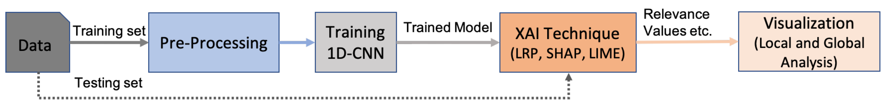
3. Proposed Approach

Our proposed approach architecture consists of two phases, as shown in Figure 1. Each of these is applied in turn to each of two datasets. The first phase consists of pre-processing and training a 1D-CNN. The proposed 1D-CNN is trained over structured data. Once the network has been trained, the trained model is used in the second phase where XAI techniques are used to visualise the important features.

Our main focus is on using 1D-CNN with LRP. However, we also showed the features selected by Shapley Additive explanation (SHAP) and Local Interpretable Model-agnostic Explanations (LIME) for comparative purposes.

3.1. First Phase

The following subsection will discuss in detail the datasets used, and the associated model training.

3.1.1. Datasets

Our aim was to create two sample models that reflect common customer-related business problems, and thus interesting explanation scenarios. We selected two scenarios: (1) The prediction of customer churn in the telecoms section and (2) the identification of fraudulent credit card transactions. To support these scenarios, we used two public structured datasets from the Kaggle website: The Telecom Customer Churn Prediction Dataset (TCCPD) and the Credit Card Fraud Detection Dataset (CCFDD). The telecom churn dataset, TCCPD, is a medium-sized dataset with meaningful feature names which can be used to give an in-depth explanation of what and why a feature is selected. In the CCFDD, the features are anonymous. It is a large and highly imbalanced dataset which make it more challenging for evaluating the performance of the proposed 1D-CNN. For all models, the datasets are divided in 80% for training and 20% for validation of the network. The results shown are based on 5-fold cross validation, using the training split. All data splits are stratified.

Telecom Customer Churn Prediction Dataset (TCCPD)

Companies want to be able to predict if a customer is at risk of leaving. Retaining an existing customer is better than getting a new customer. There are two types of customer churn—voluntary and involuntary churn. Voluntary churn is of most interest for the company as it is the individual customer’s decision to switch to another company or service provider. Understanding the factors/features that are associated with the customer leaving is important. Each record in the data [52] has initially 19 features, which when converted from categorical values to non-categorical, becomes 28 features associated with the customer, to be used for training a customer churn prediction model. These features have meaningful feature names, allowing us to interpret explanations with domain level judgement.

Credit Card Fraud Detection Dataset (CCFDD)

Financial companies dealing with credit cards have a vested interest in detecting fraudulent transactions. This highly imbalanced dataset has transactions carried out by European cardholders during September 2013. As shown in

Table 1. Details of the two datasets. Sample, positive, negative, original features, and new features are represented by Sam, +ive, −ive, O-F, and N-F, respectively.

Name	# of Samples	# +ive Sam	# −ive Sam	%+ive vs. %−ive	O-F	N-F
TCCPD	7043	1869	5174	26.58 vs. 73.42%	19	28
CCFDD	285,299	492	284,807	0.172 vs. 99.83%	30	30

, the dataset is highlighted as imbalanced. Each record contains 30 features out of which 28 are converted by Principal Component Analysis (PCA) and then labelled as V1, V2…V28. The remaining two features (time and amount) are in their original form. Each record is labelled as either 0 (normal (−ive)) or 1 (fraudulent (+ive)). Further details about this dataset are available at the Kaggle competition [53].

3.1.2. Pre-Processing

Our approach uses structured data. For ML/DL, data must be numeric in order to use it as input to the 1D-CNN network. The two used datasets are heavily imbalanced. Normalisation plays a key role in the training phase of a DL network. The following are the pre-processing steps we adopted in this work to handle the previously mentioned issues:

(1)

Convert categorical data to numerical data: Where categorical features have more than two values, we create an individual feature for each categorical value, with Yes (1) or No (0) values. The features that were numerical are normalised between 0 and 1 by zero mean and unit variance technique. In TCCPD, there are four features with categorical data. When converted, this results in nine additional features bringing our total dataset features to be 28 (Table 1).

(2)

We then apply the SMOTE [54] technique to up-sample the minority class (both datasets) in order to balance the data. SMOTE generates synthetic nearest neighbours for training instances in the minority class in the training set only.

(3)

Where numeric features ranges are wider than two-choice binary values e.g., monthly charges, the features are normalised feature-wise in the range of 0 to 1.

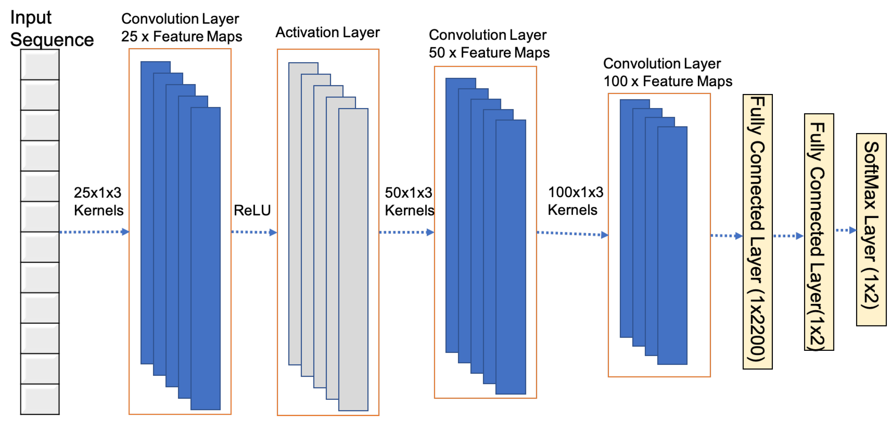
3.1.3. Training 1D-CNN

A key innovation in this work is using CNN with structured data and then explaining that deep model. We have selected to use a 1D-CNN for our model. In traditional ML, the process of selecting which features to use for a model is done using various manual steps and domain knowledge (feature engineering). Unlike traditional ML, DL learns important features as part of the training process. We use a 1D-CNN that can slide the kernel across the whole structure to learn important features.

Proposed Network Structure

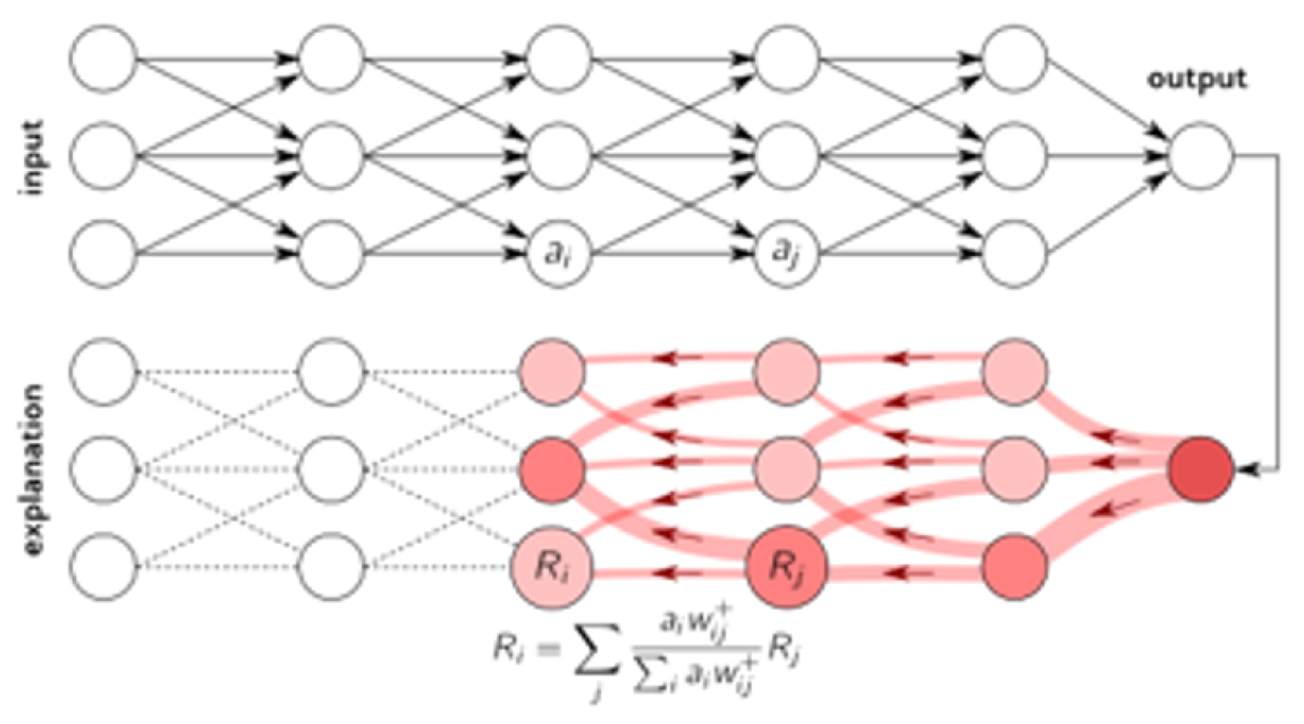
Figure 2 shows the baseline proposed 1D-CNN network structure. This network is a deep seven-layer network that contains three convolution layers (with 25, 50, and 100 kernels, respectively). The first convolution layer is followed by an activation layer. After the third convolution layer, two fully-connected layers, the first having 2200 and the second having 2 neurons are added. Finally, a SoftMax layer is added at the end. We used ReLU as an activation function.

The kernels in each layer are selected based on the concept of gradual increase or decrease rather than random as being suggested in [55]. The size of the kernel is the same for all i.e., $1\times 3$. Regarding the depth (number of layers), we have used just three, because of the data size limitation. To determine our optimal network set-up, we first tested the network with several different variations of the network structure, with the proposed model selected based on the metrics of accuracy, precision, and F1-score. We used several hyper-parameters for fine tuning the model. We used a base lr of 0.00001, batch size of 300 (unless specified differently with respective model), for a maximum iteration of 15,000.

Table 2. Proposed networks structure. Here convolution, fully connected, and output layers are represented by C, F, and O. The number shows the number of kernels/neurons in that layer.

Model Name	LR	BatchSize	Iterations	Network Structure
M-1D-CNN-1-28	0.00001	300	15,000	C25-C50-C100-F2200-O2
M-1D-CNN-2-28	0.00001	200	15,000	C25-C50-C100-F2200-F500-F10-O2
M-1D-CNN-3-16	0.00001	300	15,000	C25-C50-C100-F200-O2
M-1D-CNN-4-16	0.00001	300	15,000	C25-C50-C100-C200-F1600-F800-O2
M-1D-CNN-1-31	0.00001	300	15,000	C25-C50-C100-C200-F4400-O2
M-1D-CNN-2-31	0.0001	300	15,000	C25-C50-C100-C200-F4400-O2
M-1D-CNN-3-31	0.0001	200	15,000	C25-C50-C100-C200-F4400-O2

shows the various models that resulted from changing the base model shown in Figure 2. We will be using these variations of the base model to achieve the best model that will be used further for XAI experiments in this paper. In the Model Name column, our proposed name is in the form M-1D-CNN-n-f*. M is a short for model, n represents numbering of 1, 2, …, 5 to show that these are unique models (models are slightly different in hyper-parameters). Whereas, ‘f’ represents the number of features used as input i.e., 28 and 16.

3.2. Second Phase

XAI Technique (LRP, SHAP, and LIME)

In the second phase, once the 1D-CNN is trained, we use that trained deep model as our trial model for explainability. LRP uses the trained model to generate a heatmap based on its relevance values. Our interest in the use of heatmaps is to find and determine what set of features are the most relevant in the prediction of True Positives (1) and True Negatives (0). Furthermore, our objective is to show the important features not only for an individual sample (local analysis) but also for the whole testing set as an overall global pattern learned by the classifier (global analysis).

We have also generated heatmaps from the trained model for comparison with both SHAP and LIME. We use the default versions of LRP, SHAP, and LIME, without tuning of parameters or use of variants, in order to get a baseline comparison of the three methods. Figure 3 shows the structure of how in general LRP calculate relevance whereas Figure 4 shows the LRP heatmaps at instance and class level, with the colour scheme reflecting feature importance based on (pre-normalised) LRP values. In the following sub-sections, a brief description of how these techniques work is given.

Layer-wise Relevance Propagation (LRP): LRP is one of the main algorithms for the explainability of networks that uses the back-propagation algorithm [41]. LRP explains a classifier’s prediction specific to a given data point by attributing ‘Relevance Values’ (Ri) to important components of the input by using the topology of the trained model itself. It is efficiently utilised on images/videos and text where the output predicted value is used to calculate the relevance value for the neurons in the lower layer. The higher the impact of a neuron in the forward pass, the higher its relevance in the backward pass. This relevance calculation follows through to the input where the highly relevant neurons/features are or will have higher values compared to other neurons. As a result, when visualised, the important input neurons can be clearly highlighted based on which final decision was taken in the output layer. Figure 3 shows the flow of the relevance value calculation. LRP is currently being widely used with CNNs, and to a lesser extent for LSTM in the XAI domain. Improvements in LRP are an active area of research.

Local Interpretable Model-agnostic Explanations: LIME [32] is currently one of the most well-known methods to explain any classification model from a local point of view. This method is considered agnostic because it does not make any assumptions about how the classifier works. It simply builds a surrogate simple model, intrinsically interpretable, such as a linear regression model around each prediction between the input variables and the corresponding outcome variables. The use of a simple model in a local way allows for easier interpretation of the behaviour of the classification model in the vicinity of the instance being predicted. LIME attempts to understand the classification model by perturbing the input variables of a data sample and understanding how the predictions change.

In a simplified way, LIME works by first generating random perturbations (fake observations) around the instance to be explained (original instance). Secondly, it calculates a similarity distance between the perturbations and original instance (e.g., Euclidean distance). Thirdly, it gets the predictions for the perturbations. Followed by picking a set of perturbations with better similarity scores and calculate weights (distance scaled to [0, 1]) that represent the importance of these perturbations in respect to the original instance. Once perturbations, predictions, and weights have been calculated, it builds a weighted linear regression model, where the coefficients of this simple model will help to explain how changes in the explanatory variables affect the classification outcome for the instance that wishes to be explained. LIME focuses on training local surrogate models to explain individual predictions. Hence, it can be applied to any DL model. However, in terms of time complexity, it is simpler than SHAP, but yet requires sometime to train.

Shapley Additive Explanations (SHAP): SHAP is an approach based on game theory to explain the output of any (but mainly traditional) ML models [33]. It uses Shapley values from game theory to give a different perspective to interpret black box models by connecting the optimal credit allocation with local explanations and their related extensions. This technique works as follows: To get the importance of feature $X_i$, it first takes all subsets of features S, other than $X_i$. It then computes the effect of the output predictions after adding $X_i$ to all the subsets previously extracted. Finally, it combines all the contributions to compute the marginal contribution of the feature. To avoid recalculation of these subsets, SHAP does not retrain the model with the feature in question left out. It just replaces it with the average value of the feature and generates the predictions. The features which are strongly influential to the model output from the input values are shown. Typically, these influential features are shown in red and other less influential features in blue. This provides a useful clear explanation for simpler models. It is currently (as of this document date) limited to application to traditional ML models due to its time complexity. In this work, we used kernel SHAP. Whilst a line of investigation could focus on other types of SHAP in order to change the time complexity, we note that is well documented in general that SHAP is a time-intensive technique.

3.3. Validating the Correctness of LRP’s Highlighted Subset of Features

We used three XAI techniques for an explanation of features. LRP uses a heatmap to highlight the processed features that have most contributed to the model decision. To validate that the set of features highlighted by XAI techniques (mainly LRP) are genuinely influential on model decisions, we use the highlighted features, with the original dataset labels, to train a simple classifier e.g., Logistic Regression, RF, SVM, and see whether the 1D-CNN and/or some simple classifier can generate better or equal results with the subset of discriminative features highlighted by XAI techniques. Achieving comparative prediction results will prove that the features highlighted by LRP represent the decision-driving features in the dataset. Rather than manually selecting the highlighted features in the heatmaps, we propose a method that takes account of LRP values for each instance in the dataset, summing to a global ranking for each feature at a dataset level. Our approach assumes that all classes are equal weight—i.e., that both labels TP and TN are of equal importance when producing the final feature ranking. In this approach, we first ranked the features and then did a subset selection of features using a threshold as explained below: Let M be an $nxm$ matrix composed by row vectors $v_i=\langle l_1^i,...,l_m^i\rangle$, $i=\{1,...,n\}$. Each vector $v_i$ represents the LRP values ($l_j^i$) of each one of the n records from the test set for each feature j of the model, where $j=\{1,...m\}$. For each feature j (column), the coefficient of variation $C{V}_j=\frac{sd\left({\langle l_j^1,...,l_j^n\rangle }^T\right)}{mean\left({\langle l_j^1,...,l_j^n\rangle }^T\right)}$ is calculated. Then the threshold is the mean (${\mu }_j$) of the feature j with the smallest positive $CV$. The idea is to define a value that represents the positive mean of the feature with the lowest dispersion. Initially, the selection was done by visualising the boxplot chart by columns of the matrix of LRP values. We then set out the method in the following steps to pave the way to automation:

1.

Set a threshold value t to be used. This threshold represents a cut-off LRP value above which a feature is determined to have contributed to an individual correct test instance.

2.

Select all instances (with their LRP vectors) that were correctly classified as True Positive (TP).

3.

Apply the threshold t to the relevance values of each feature j of a record in the true positives and true negatives, converting the feature value to 1 if at or above the threshold, else 0. This is $\left\{l_j^i\right\}\ge t\Rightarrow 1$ and $\left\{l_j^i\right\}<t\Rightarrow 0$.

4.

Sum the rows which have had features converted with 0 or 1, resulting in one vector r of dimension m, where m is the number of features.

$r=\langle {\sum }_{i=1}^n{l}_1^i...{\sum }_{i=1}^n{l}_j^i...{\sum }_{i=1}^n{l}_m^i\rangle$

5.

Sort this vector based on the summed values for the features, to produce a numeric ranking of features

6.

Repeat Steps 2–5 for the True Negative (TN) records

7.

Select a total of 16 features (top 8 from TP vector and top 8 from TN vector). In case of an odd number, more are selected from TP (one less from TN features).

This is the approach that we have adopted for the thresholding and selection of the features. However, more sophisticated techniques, such as allowance for class weighting or merging of LRP values across classes prior to ranking, can be adopted for selecting the features. The relevance values are all in the range of 0 and 1 (note, the relevance values are all in 0 and 1, whereas the heatmaps in Figure 4 and Figure 5 shows between −1 and 1, this is only for better visualisation purposes. Otherwise the values are all in 0 and 1). Therefore, the threshold must be with in the range of 0 and 1 e.g., 0.4, 0.5. Considering a threshold greater than 0.6 will give the most discriminative features for predicting the TPs but may lose some supporting features that will help in differentiating them from TNs. On the other hand, selecting a threshold smaller than 0.5 may result in too many features as a subset, which might again increase the ambiguity and may affect the decision and result in higher FNs or FPs. The number ‘16’ in the last step is not constant, rather it can be tuned considering the number of features in the dataset in question. A dataset with 100 features versus 50 features might have a different subset of discriminative features that will result in optimal performance. We also note that there is a lack of strongly negative LRP feature patterns on the global heatmaps. This is the nature of these datasets, and the resultant models. With different datasets/scenarios, where there is an occurrence of strongly negative LRP feature patterns, the threshold can be adjusted to ensure the important contribution of these features. Here by negative we mean the features that have negative impact/influence on the decisions or the features that are the cause of a wrong result. Next, phase optimisation will examine this further. Eventually we will show ranked example of the TP case for both datasets in Section 4. A point to highlight is that we choose downstream classification as we are looking for evidence that we have a good feature set, not an empirical feature selection comparison. A wider exercise of comparison to other feature selection methods can be done later.

4. Results

Every DL network needs to be tuned before one arrives at an optimal model. We trained a similar 1D-CNN network on both datasets. However, some changes were needed in the hyper-parameters (added in following section) to get optimal results. This is mainly because of the size and imbalance nature of the data distribution of the classes. Furthermore, we worked upon several models for achieving the best results and compared the results internally (trained by ourselves) for a 1D-CNN model versus several ML classifiers (e.g., Logistic Regression, Random Forest). This is because the dataset was mainly used in a competition on Kaggle and very few papers have used the data.

The following subsections will:

(a)

Show that 1D-CNN can work on structured data and its performance for both the datasets will be shown in the form of accuracy, precision, recall, specificity, and F1-measure,

(b)

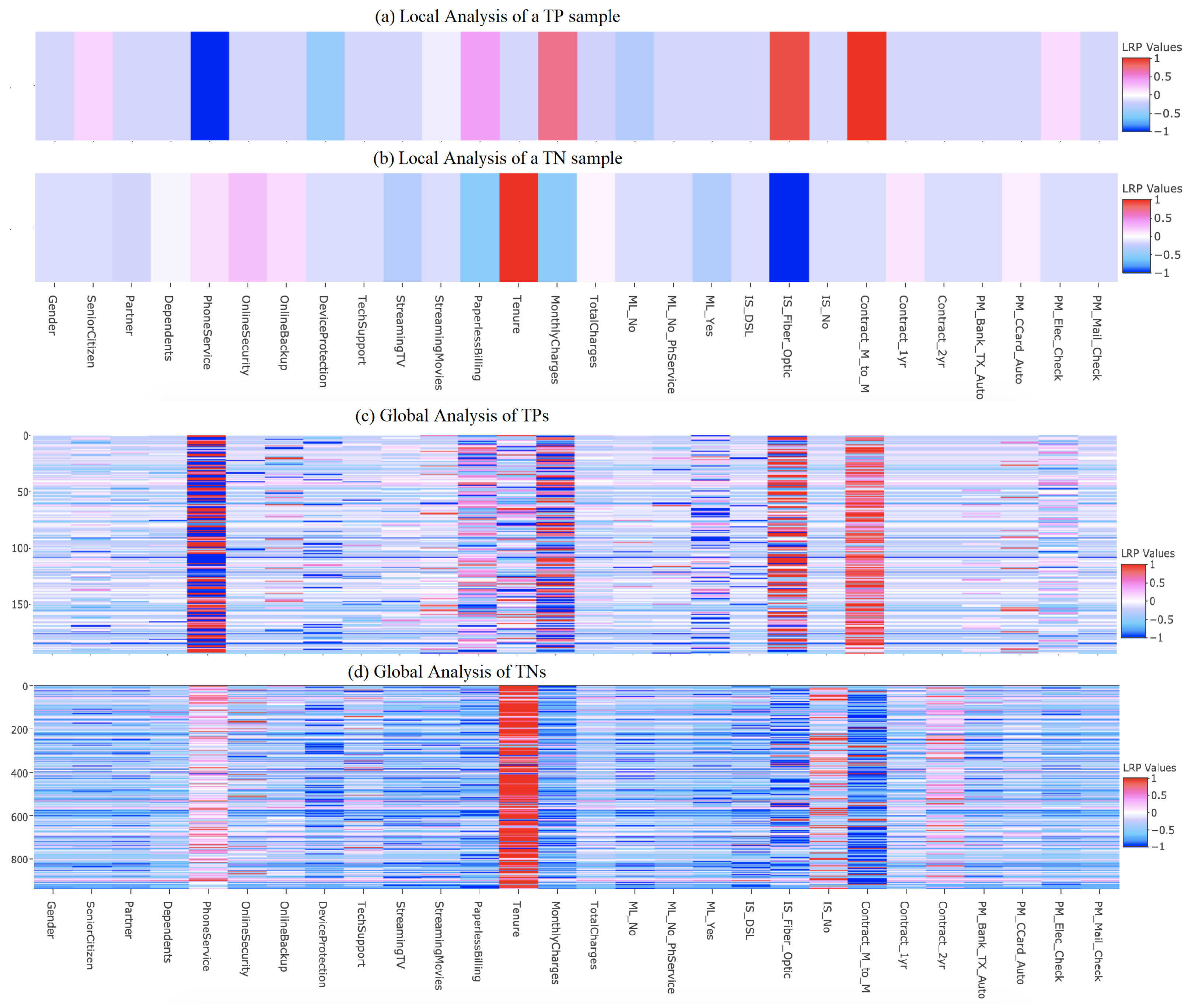
Discuss the visualised features in a heatmap that play a key role in a decision and assessing the results qualitatively (only on telecom churn dataset because the features of CCFDD are anonymous),

(c)

Compare the highlighted features from the heatmaps of LRP, SHAP, and LIME,

(d)

Validate that the selected subset of features are really important and can show good results when used as input to a simple classifier (done over TCCPD because we know the domain knowledge and the features names),

(e)

Finally, compare the performance with other techniques.

4.1. Performance of 1D-CNN on Structured Data

The previous highest accuracy on the TCCPD was 82.94% [56], achieved with an XGboost classifier having min-max scaler for pre-processing of the 28 features. This result is reported without using cross validation. Looking at

Table 3. Comparison of ours (with *) vs. other models on TCCDD. Accuracy, precision, specificity, and cross-validation are represented by Acc, Preci, Speci, and Cross-V, respectively.

Model Name	Train/Test	Acc	Preci	Recall	Speci	F1-Score	Cross-V
M-1D-CNN-1-28 *	80/20	0.8264	0.7011	0.6189	0.9028	0.657	Yes
M-1D-CNN-2-28 *	80/20	0.8041	0.6727	0.5497	0.8985	0.5978	Yes
Logistic Regression-28 *	80/20	0.7993	0.6616	0.5221	0.9015	0.583	Yes
Decision Tree-28 *	80/20	0.7864	0.6875	0.3794	0.9363	0.4881	Yes
Random Forest-28 *	80/20	0.7773	0.7172	0.2842	0.9588	0.4066	Yes
SVM Linear-28 *	80/20	0.7973	0.656	0.5209	0.8991	0.5802	Yes
SVM RBF-28 *	80/20	0.7785	0.6358	0.4159	0.9122	0.5023	Yes
XG Boost-28 *	80/20	0.7649	0.5727	0.4956	0.8641	0.5311	Yes
Results in Literature	–	–	–	–	–	–	–
Logistic Regression [62]	75/25	0.8003	0.6796	0.5367	–	0.5998	No
Random Forest [62]	75/25	0.7975	0.6694	0.4796	–	0.569	No
SVM RBF [62]	75/25	0.7622	0.5837	0.5122	–	0.5457	No
Logistic Regression [56]	70/30	0.8075	–	–	–	–	No
Random Forest [56]	80/20	0.8088		–	–	–	No
SVM	80/20	0.8201	–	–	–	–	No
ADA Boost [56]	80/20	0.8153	–	–	–	–	No
XG Boost-28 [56]	80/20	0.8294	–	–	–	–	No
Logistic Regression [63]	80/20	0.8005	–	–	–	–	No
Reduced Features Results	–	–	–	–	–	–	–
M-1D-CNN-4-16 *	80/20	0.8462	0.7339	0.6718	0.9104	0.7014	Yes
M-1D-CNN-5-16 *	80/20	0.8554	0.7399	0.713	0.908	0.726	Yes
Logistic Regression-16 *	80/20	0.7996	0.6633	0.52	0.9026	0.5823	Yes
Decision Tree-16 *	80/20	0.7871	0.6911	0.3788	0.9374	0.4886	Yes
Random Forest-16 *	80/20	0.7807	0.7058	0.3139	0.9521	0.4337	Yes
SVM-16 *	80/20	0.7986	0.6571	0.5278	0.8984	0.5849	Yes
XG Boost-16 *	80/20	0.7618	0.5645	0.5035	0.8569	0.532	Yes

, our models gained results less than that mentioned in the above point. However, with M-1D-CNN-1-2$8^{*}$, we achieved 82.64% accuracy and a decent precision of 71.11%. Our highest accuracy with traditional ML classifiers is 79.93% with precision of 66.16% using logistic regression on all the 28 features. Random forest is the classifier which gave 71.72% of precision with 77.73% accuracy.

Table 4. Comparison of our 1D-CNN (with *) performance on CCFDD against published results.

Model Name	Train/Test	Acc	Prec	Recall	Spec	F1-Score	Cross-V
M-1D-CNN-1-31 *	80/20	0.9991	0.6732	0.9520	0.9992	0.7866	Yes
M-1D-CNN-2-31 *	80/20	0.9989	0.6507	0.8779	0.9992	0.7446	Yes
M-1D-CNN-3-31 *	80/20	0.9987	0.6079	0.8553	0.9990	0.7037	Yes
Logistic Regression-31 *	80/20	0.9229	0.0201	0.9044	0.9230	0.0393	Yes
Decision Tree-31 *	80/20	0.9651	0.0442	0.8762	0.9652	0.0840	Yes
Random Forest-31 *	80/20	0.9946	0.2232	0.8579	0.9948	0.3533	Yes
Gaussian NB-31 *	80/20	0.9748	0.0550	0.8474	0.9751	0.1033	Yes
Logistic Regression [57]	80/20	0.81	0.76	0.9	–	0.82	No
Isolation Forest [59]	70/30	0.997	–	–	–	0.63	No
Local Outlier Forest [59]	70/30	0.996	–	–	–	0.51	No
SVM [59]	70/30	0.7009	–	–	–	0.41	No

shows the results we achieved with the proposed model on the credit-card fraud dataset. Our model (M-1D-CNN-1-3$1^{*}$) achieved best results in terms of accuracy. This data is highly imbalanced, and due to its complexity, the precision is slightly low in comparison to [57]. However, its overall accuracy is less than ours by a margin. Our model also shows better results compared to others reported in [58,59]. These two models (M-1D-CNN-1-2$8^{*}$ and M-1D-CNN-1-3$1^{*}$) are used along with LRP to visualise the features of TCCPD and CCFDD datasets, respectively.

Although 1D-CNN for structured data shows a good classification result, however a possible limitation where 1D-CNN may struggle will be the lack of translation invariant in the the situation where different features have similar value ranges and repeats/overlaps in the same order in various positions. A potential solution will be adding positional information in the form of unique delimiters that will make sure that features with the same value will not be mixed up with one another as the associated feature map will include the unique ID in some way considering that even if the features are shuffled the unique features will also be moved with respective real features.

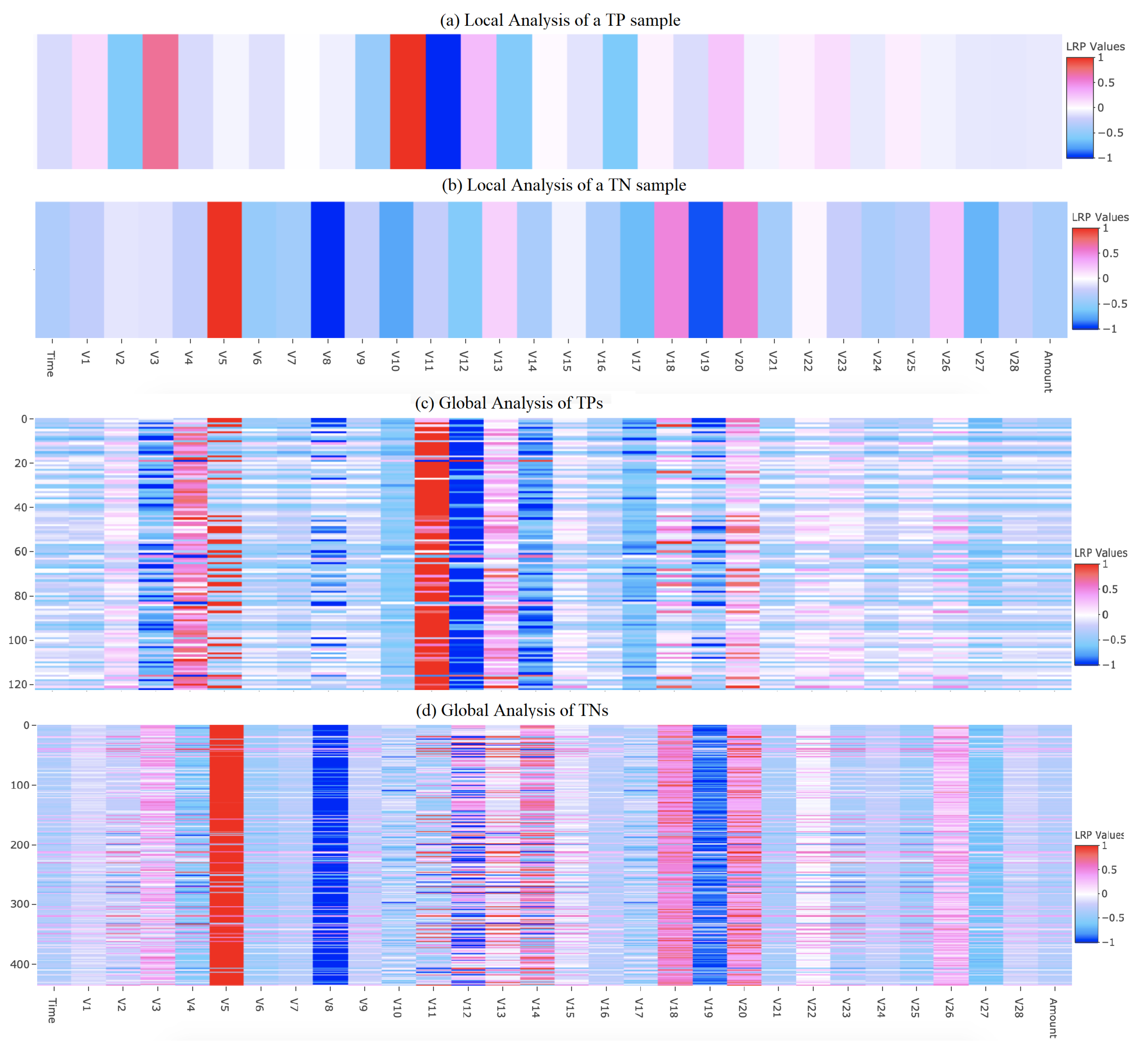
4.2. Visualising Local and Global Heatmaps of Features Using LRP

The main objective of XAI in this work is to see how or why a deep network gave a specific decision (TP, TN, FP, or FN). Figure 4a shows a heatmap generated by LRP for local interpretation of a single record that resulted in TP. The heatmap clearly shows that because of features such as the customer being a senior citizen (SeniorCitizen), monthly contract (contract_M_to_M), Fiber optic internet (IS_Fiber_Optic), high monthly charges (MonthlyCharges), and no phone service (PhoneService) it is predicted that this customer is going to churn. Based on our research in the domain/general business domain, it is known and/or learned that a customer is more likely to churn if the contract is monthly, having no phone service, and with high monthly charges. To retain the customer, it is suggested that the company reduces some charges by reducing some features but offers a yearly or biyearly contract so as to retain the customer for a longer term. Hence, although it is not being tested/validated by us, it is still known and understandable by the companies (e.g., VirginMedia Ireland Mobile and Internet [60] as they offer lower charges but longer contracts as well as introducing fibre connections rather than old technology.

Figure 4b shows the local analysis of a record which will not churn. The heatmap shows the features for a customer who will not churn, and is not a senior citizen, has online security, a contract of one year without fiber optic, with several other features but fewer monthly charges. Figure 4c shows a clear pattern for all the correctly classified TP samples in the testing set, highlighting the important features that play a key role in the model decision towards being marked as TP. The same applies in the case for TNs as shown in Figure 4d.

This ability to understand model decisions at a class level has a tangible business use case. In our TCCPD business domain example, understanding TP and TN can help a company/data scientist in increasing the revenue by retaining the customers—supporting the well-known maxim that in business, it is easier to keep a customer than to find a new one. On the other hand, understanding and recognising the key features for the local and global analysis of FP and FN samples may help data scientists to avoid or reduce the discrepancy in the data results in miss-classifications by the model. Our demonstrator [61] also highlights heatmaps for FP/FNs and the features that play key roles in generating incorrect predictions. This is helpful for understanding useful information about the data and enhancing the trained model information e.g., to avoid redundant or ambiguous features that impact the performance of the deep learning models. Figure 5 shows the heatmaps for local (individual) and global (all) TP and TN samples in a CCFDD testing set.

4.3. Qualitative Comparison of Heatmaps from LRP, SHAP, and LIME

One of the main ideas of our work was to show that LRP can perform well for explainability of the deep model in various forms. SHAP and LIME are two other common techniques used for explainability. Using LRP as the baseline explainability technique, we demonstrate advantages of LRP because it highlights the same features as discriminative as those of SHAP and LIME but in far less execution time.

Table 5. Ranked feature comparison for LRP, SHAP, and LIME over the Telecom Churn dataset.

	Contract_M_to_M	PhoneService	IS_Fiber_Optic	MonthlyCharges	PaperlessBilling	Tenure	PM_CCard_Auto	OnlineBackup	StreamingMovies	ML_Yes	PM_Elec_Check	ML_No_PhService	ML_No	PM_Bank_TX_Auto	StreamingTV	TechSupport	DeviceProtection	Dependents	OnlineSecurity	Partner	SeniorCitizen	PM_Mail_Check	TotalCharges	IS_DSL	IS_No	Contract_1yr	Contract_2yr	Gender
LRP	28	27	26	25	24	23	22	21	20	19	18	17	16	12	12	12	12	1	1	1	1	1	1	1	1	1	1	1
LIME	26	22	25	1	1	24	1	1	1	1	1	1	1	1	1	21	1	1	23	1	1	1	1	1	26	1	26	1
SHAP	26	25	28	23	1	27	1	1	1	1	1	1	1	1	1	1	1	1	1	1	24	1	1	1	1	1	1	1

and

Table 6. Ranked feature comparison for LRP, SHAP, and LIME over the credit card dataset.

	V11	V4	V5	V20	V13	V18	V14	V12	V3	V26	V22	V2	V6	V7	V8	V9	V10	V1	Amount	V28	V15	V16	V17	V19	V21	V23	V24	V25	V27	Time
LRP	30	29	28	27	26	25	24	23	21	21	20	1	1	1	1	1	1	1	1	1	1	1	1	1	1	1	1	1	1	1
LIME	30	25	1	1	23	1	27	29	24	1	1	1	1	1	1	1	28	1	1	1	1	1	25	1	1	1	1	1	1	1
SHAP	28	27	1	1	25	1	28	30	24	1	1	1	1	1	1	1	23	1	1	1	1	1	26	1	1	1	1	1	1	1

show the features ranked in descending order for LRP, SHAP, and LIME from the model trained on TCCPD and CCFDD, respectively. The ranking is done based on the approach explained in Section 3.3. The value 28 shows that the feature is highly discriminative and is considered important whereas 1 means having low importance in the tables. The features are sorted in descending order of LRP ranking, whilst showing the other rankings of LIME and SHAP with respect to the LRP ranking. As we have taken top and bottom eight features from TP and TN each, therefore, if we consider the important (top) features in the first row of Table 5, and similarly for corresponding SHAP and LIME, we can see that the features ranked high (e.g., with 28, 27) in LRP are mostly ranked high in SHAP and LIME as well (e.g., Contract_M_M, PhoneService, Tenure, IS_Fiber_Optic, Monthly charges). Five out of eight features are common for all three. In addition, the time taken by LRP running on CPU (MacBook Pro with Intel Core i5, 2.3 GHz 1 Processor with 2 Cores, and 16 GB RAM) is 1–2 s to generate a heatmap for a single record at test time which is far lower than the time taken by LIME (22 s) and SHAP (108 s). This shows that LRP is faster. We also show in the section that it selects a highly discriminative feature set, that if used with a simple classifier, will generate a similar or better performance. This is possible because the ambiguous or redundant features are removed which were confusing the system. The SHAP and LIME code can be slightly optimised by either changing some of its parameters (for example the size of the neighbourhood (we used default of 10, if we increase it increases the time it takes), parameters for regularisation) however, it takes more time compared to LRP.

4.4. Validation of the Subset of LRP Highlighted Features Importance

It is important to verify that the features highlighted as important by LRP are genuinely pivotal in driving the model decisions. Therefore, we use the subset of important features highlighted by LRP as input to traditional ML techniques (e.g., logistic regression, random forest) and proposed 1D-CNN. The last five rows in Table 3 show that using features generated from LRP values did not yield good results with traditional ML classifiers. However, we achieved good results with the deep 1D-CNN (M-1D-CNN-4-16* and M-1D-CNN-5-16*) as shown in Table 3. The interesting point is that our 1D-CNN for LRP surpassed the existing kernel [59] results both in terms of accuracy and precision while trained on this subset of features. We achieved a highest accuracy of 85.54% with a precision of 73.995% and a F1-score of 72.603%. Moreover, we achieved higher a F1-score of 73.23% from the model with using LRP values as features using SMOTE for balancing the data and with batch size 200 and a LR of 0.00001. A key point to note is that using features derived from LRP values, all 1D-CNN models gave results close to 83%. In addition, it is to clarify that the main cause of improvement is the proposed strategy which achieved a high F1-score i.e., 72.603%. Whereas, using SMOTE gave an additional enhancement of 0.63% to get a higher F1-score i.e., 73.23%. SMOTE without the proposed strategy was not able to achieve the achieved F1-score.

The used subset of features contain 16 features. These are selected from the LRP values generated by the process as explained in Section 3.3. The good performance with this subset of features proves that the highlighted features are important and can generate an almost similar result through a simple classifier instead of a DL model. Hence, if needed in a situation where memory and processing is an issue e.g., when deployed in IoT or on edge device, a smaller simple classifier can be used rather than a deep neural network.

4.5. Comparison with State-of-the-Art

Table 3 shows comparison of the results achieved by the proposed model against others. In addition, it also contain the results from a traditional ML trained by other researchers in research articles and on the Kaggle competition webpage. The ‘*’ represents the models (both traditional ML) we trained and tested ourselves with similar data. Many of the results were not based on 5-fold cross validation. To get a fair results comparison, we retrained same techniques using 5-fold cross validation. One point to highlight is that the published state-of-the-art is only available for the actual original model classification performance i.e., We have no state-of-the-art results for the correctness of features highlighted by LRP.

The results showed that our results from 1D-CNN (M-1D-CNN-1-28*) in the case of using all 28 features is lower than XG-Boost [56] by 0.0003. However, for the same XG Boost-28* when we trained and calculated a performance after 5-cross validation, it showed 0.0615 fewer performance than our best model (M-1D-CNN-1-28*) with 28 features as input.

In terms of precision, Random Forest-28* achieved the highest precision of 0.7172, which is 0.0478 and 0.0161 higher than Random Forest results reported in [62] and our M-1D-CNN-1-28* model, respectively. However, in terms of F1-score, our model showed better result than that of Random Forest-28* and reported by [62] by 0.2514 and 0.088, respectively.

The state-of-the-art results are achieved when we use our proposed model for selecting a subset of features and then using those selected features as input to the same networks (1D-CNN and traditional ML techniques) to train and test. Our model M-1D-CNN-5-16* achieved a 0.8554 accuracy, 0.7399 precision, and 0.7260 F1-score, which are higher than all other models at a good margin. This shows that XAI as an approach for subset selection of discriminative features can give us almost equal or better results with both the proposed 1D-CNN model and traditional ML techniques. This can be used as a strategy of first using DL, and then when we have the reduced feature set, using those with a simple classifier which paves the way to investigating this approach for use on embedded or edge devices where there are limitations on memory.

5. Conclusions

We provided the first application of 1D-CNN and LRP on structured data. In terms of accuracy, precision, and F1-score performance, our deep network performs marginally below the benchmark methodology reported in state-of-the-art on the same data by a small fraction but achieved higher when we used cross-validation on the same model. However, more importantly, we took the initiative for using 1D-CNN+LRP on structured data. Using the approach of 1D-CNN+LRP for validating the subset of features highlighted by LRP as important, the reduced feature set used to train a model can give state-of-the-art performance. Hence, we initiated a new area of research for XAI as a tool for feature subset selection. However, the comparison of downstream classification for the selected features versus the full dataset indicates that LRP has selected informative features, as classification results are maintained or improved but to further verify LRP’s potential for feature selection, comparison with other feature selection techniques is required. The proposed approach enhances performance in terms of accuracy, precision, F1-score, and computation time. It also substantially reduced the number of features to be used in a deployed system where resources are limited e.g., an edge device. For future work, we plan to do further analysis on exploring the possibility of whether a 1D-CNN can be made for structured data in a translational invariant model. In addition, exploring the system with other datasets (e.g., UCI Benchmark Repository) and explainability techniques e.g., DeepLIFT, LORE, MAPLE, L2X, as well as adopt cross validation approach for validating the selected features.

References

1. Gunning, D.; Aha, D. DARPA’s Explainable Artificial Intelligence (XAI) Program. AI Mag. 2019, 40, 44–58. [Google Scholar]
2. Krizhevsky, A.; Sutskever, I.; Hinton, G.E. ImageNet Classification with Deep Convolutional Neural Networks. Adv. Neural Inf. Process. Syst. 2012, 25, 1097–1105. [Google Scholar] [CrossRef]
3. Kolesnikov, A.; Beyer, L.; Zhai, X.; Puigcerver, J.; Yung, J.; Gelly, S.; Houlsby, N. Large Scale Learning of General Visual Representations for Transfer. arXiv 2019, arXiv:1912.11370. [Google Scholar]
4. Xie, S.; Girshick, R.; Dollar, P.; Tu, Z.; He, K. Aggregated Residual Transformations for Deep Neural Networks. In Proceedings of the 2017 IEEE Conference on Computer Vision and Pattern Recognition (CVPR), Honolulu, HI, USA, 21–26 July 2017; pp. 5987–5995. [Google Scholar] [CrossRef] [Green Version]
5. Liu, Y.; Wang, Y.; Wang, S.; Liang, T.; Zhao, Q.; Tang, Z.; Ling, H. CBNet: A Novel Composite Backbone Network Architecture for Object Detection. arXiv 2019, arXiv:1909.03625. [Google Scholar] [CrossRef]
6. Howard, A.; Sandler, M.; Chu, G.; Chen, L.C.; Chen, B.; Tan, M.; Wang, W.; Zhu, Y.; Pang, R.; Vasudevan, V.; et al. Searching for MobileNetV3. arXiv 2019, arXiv:1905.02244. [Google Scholar]
7. Li, B.; Wu, W.; Wang, Q.; Zhang, F.; Xing, J.; Yan, J. SiamRPN++: Evolution of Siamese Visual Tracking with Very Deep Networks. arXiv 2018, arXiv:1812.11703. [Google Scholar]
8. Silver, D.; Huang, A.; Maddison, C.J.; Guez, A.; Sifre, L.; van den Driessche, G.; Schrittwieser, J.; Antonoglou, I.; Panneershelvam, V.; Lanctot, M.; et al. Mastering the game of Go with deep neural networks and tree search. Nature 2016, 529, 484–489. [Google Scholar] [CrossRef]
9. Liu, J.; Chao, F.; Lin, Y.C.; Lin, C.M. Stock Prices Prediction using Deep Learning Models. arXiv 2019, arXiv:1909.12227. [Google Scholar]
10. Fang, X.; Yuan, Z. Performance enhancing techniques for deep learning models in time series forecasting. Eng. Appl. Artif. Intell. 2019, 85, 533–542. [Google Scholar] [CrossRef]
11. Gasparin, A.; Lukovic, S.; Alippi, C. Deep Learning for Time Series Forecasting: The Electric Load Case. arXiv 2019, arXiv:1907.09207. [Google Scholar] [CrossRef]
12. Liu, Y.; Kohlberger, T.; Norouzi, M.; Dahl, G.E.; Smith, J.L.; Mohtashamian, A.; Olson, N.; Peng, L.H.; Hipp, J.D.; Stumpe, M.C. Artificial intelligence–based breast cancer nodal metastasis detection insights into the black box for pathologists. Arch. Pathol. Lab. Med. 2019, 143, 859–868. [Google Scholar] [CrossRef] [Green Version]
13. Baehrens, D.; Schroeter, T.; Harmeling, S.; Kawanabe, M.; Hansen, K.; Müller, K.R. How to Explain Individual Classification Decisions. J. Mach. Learn. Res. 2010, 11, 1803–1831. [Google Scholar]
14. Malgieri, G. Automated decision-making in the EU Member States: The right to explanation and other “suitable safeguards” in the national legislations. Comput. Law Secur. Rev. 2019, 35, 105327. [Google Scholar] [CrossRef]
15. Tjoa, E.; Guan, C. A Survey on Explainable Artificial Intelligence (XAI): Towards Medical XAI. arXiv 2019, arXiv:1907.07374. [Google Scholar] [CrossRef]
16. Selvaraju, R.R.; Cogswell, M.; Das, A.; Vedantam, R.; Parikh, D.; Batra, D. Grad-CAM: Visual Explanations from Deep Networks via Gradient-Based Localization. In Proceedings of the IEEE International Conference on Computer Vision, Venice, Italy, 22–29 October 2017; pp. 618–626. [Google Scholar]
17. Mitchell, M.; Wu, S.; Zaldivar, A.; Barnes, P.; Vasserman, L.; Hutchinson, B.; Spitzer, E.; Raji, I.D.; Gebru, T. Model Cards for Model Reporting. In Proceedings of the Conference on Fairness, Accountability, and Transparency—FAT* ’19, Atlanta, GA, USA, 29–31 January 2019; pp. 220–229. [Google Scholar]
18. Guidotti, R.; Monreale, A.; Ruggieri, S.; Turini, F.; Giannotti, F.; Pedreschi, D. A survey of methods for explaining black box models. ACM Comput. Surv. 2018, 51, 1–42. [Google Scholar] [CrossRef] [Green Version]
19. Barredo Arrieta, A.; Díaz-Rodríguez, N.; Del Ser, J.; Bennetot, A.; Tabik, S.; Barbado, A.; Garcia, S.; Gil-Lopez, S.; Molina, D.; Benjamins, R.; et al. Explainable Artificial Intelligence (XAI): Concepts, taxonomies, opportunities and challenges toward responsible AI. Inf. Fusion 2020, 58, 82–115. [Google Scholar] [CrossRef] [Green Version]
20. Shrikumar, A.; Greenside, P.; Kundaje, A. Learning Important Features Through Propagating Activation Differences. In Proceedings of the 34th International Conference on Machine Learning, Sydney, Australia, 6–11 August 2017; Precup, D., Teh, Y.W., Eds.; International Convention Centre: Sydney, Australia, 2017; Volume 70, pp. 3145–3153. [Google Scholar]
21. Guo, W.; Mu, D.; Xu, J.; Su, P.; Wang, G.; Xing, X. LEMNA: Explaining Deep Learning Based Security Applications. In Proceedings of the 2018 ACM SIGSAC Conference on Computer and Communications Security, Toronto, ON, Canada, 15–19 October 2018; Association for Computing Machinery: New York, NY, USA, 2018; pp. 364–379. [Google Scholar] [CrossRef]
22. Plumb, G.; Molitor, D.; Talwalkar, A. Supervised Local Modeling for Interpretability. arXiv 2018, arXiv:1807.02910. [Google Scholar]
23. Guidotti, R.; Monreale, A.; Ruggieri, S.; Pedreschi, D.; Turini, F.; Giannotti, F. Local Rule-Based Explanations of Black Box Decision Systems. arXiv 2018, arXiv:1805.10820. [Google Scholar]
24. Chen, J.; Song, L.; Wainwright, M.; Jordan, M. Learning to explain: An information-theoretic perspective on model interpretation. In Proceedings of the International Conference on Machine Learning, Stockholm, Sweden, 10–15 July 2018; pp. 883–892. [Google Scholar]
25. Lundberg, S.M.; Erion, G.; Chen, H.; DeGrave, A.; Prutkin, J.M.; Nair, B.; Katz, R.; Himmelfarb, J.; Bansal, N.; Lee, S.I. Explainable AI for Trees: From Local Explanations to Global Understanding. arXiv 2019, arXiv:1905.04610. [Google Scholar] [CrossRef]
26. Gilpin, L.H.; Bau, D.; Yuan, B.Z.; Bajwa, A.; Specter, M.; Kagal, L. Explaining Explanations: An Overview of Interpretability of Machine Learning. In Proceedings of the 2018 IEEE 5th International Conference on Data Science and Advanced Analytics (DSAA), Turin, Italy, 1–3 October 2018; pp. 80–89. [Google Scholar]
27. El-assady, M.; Jentner, W.; Kehlbeck, R.; Schlegel, U. Towards XAI: Structuring the Processes of Explanations. In Proceedings of the ACM Workshop on Human-Centered Machine Learning, Glasgow, UK, 4 May 2019. [Google Scholar]
28. Watson, D.S.; Krutzinna, J.; Bruce, I.N.; Griffiths, C.E.; McInnes, I.B.; Barnes, M.R.; Floridi, L. Clinical applications of machine learning algorithms: Beyond the black box. BMJ 2019, 364, l886. [Google Scholar] [CrossRef] [PubMed] [Green Version]
29. Mittelstadt, B.; Russell, C.; Wachter, S. Explaining explanations in AI. In Proceedings of the 2019 Conference on Fairness, Accountability, and Transparency, Atlanta, GA, USA, 29–31 January 2019; pp. 279–288. [Google Scholar]
30. Samek, W.; Müller, K.R. Towards Explainable Artificial Intelligence. In Lecture Notes in Computer Science, Proceedings of the Explainable AI: Interpreting, Explaining and Visualizing Deep Learning; Springer: Cham, Switzerland, 2019; pp. 5–22. [Google Scholar]
31. Lapuschkin, S.; Wäldchen, S.; Binder, A.; Montavon, G.; Samek, W.; Müller, K.R. Unmasking Clever Hans predictors and assessing what machines really learn. Nat. Commun. 2019, 10, 1096. [Google Scholar] [CrossRef] [PubMed] [Green Version]
32. Ribeiro, M.T.; Singh, S.; Guestrin, C. “Why Should I Trust You?”: Explaining the Predictions of Any Classifier. In Proceedings of the 22nd ACM SIGKDD International Conference on Knowledge Discovery and Data Mining, San Francisco, CA, USA, 13–17 August 2016; pp. 1135–1144. [Google Scholar]
33. Lundberg, S.M.; Lee, S.I. A Unified Approach to Interpreting Model Predictions. In Advances in Neural Information Processing Systems 30; Guyon, I., Luxburg, U.V., Bengio, S., Wallach, H., Fergus, R., Vishwanathan, S., Garnett, R., Eds.; Curran Associates, Inc.: New York, NY, USA, 2017; pp. 4765–4774. [Google Scholar]
34. Tian, Y.; Liu, G. MANE: Model-Agnostic Non-linear Explanations for Deep Learning Model. In Proceedings of the 2020 IEEE World Congress on Services (SERVICES), Beijing, China, 18–23 October 2020; pp. 33–36. [Google Scholar] [CrossRef]
35. Simonyan, K.; Vedaldi, A.; Zisserman, A. Deep inside convolutional networks: Visualising image classification models and saliency maps. In Proceedings of the 2nd International Conference on Learning Representations, ICLR 2014-Workshop Track Proceedings, Banff, AB, Canada, 14–16 April 2014; pp. 1–8. [Google Scholar]
36. Arras, L.; Montavon, G.; Müller, K.R.; Samek, W. Explaining Recurrent Neural Network Predictions in Sentiment Analysis. arXiv 2018, arXiv:1706.07206. [Google Scholar]
37. Zeiler, M.D.; Krishnan, D.; Taylor, G.W.; Fergus, R. Deconvolutional networks. In Proceedings of the 2010 IEEE Computer Society Conference on Computer Vision and Pattern Recognition, San Francisco, CA, USA, 13–18 June 2010. [Google Scholar]
38. Zeiler, M.D.; Taylor, G.W.; Fergus, R. Adaptive deconvolutional networks for mid and high level feature learning. In Proceedings of the 2011 International Conference on Computer Vision, Barcelona, Spain, 6–13 November 2011; pp. 2018–2025. [Google Scholar]
39. Zeiler, M.D.; Fergus, R. Visualizing and understanding convolutional networks. In Lecture Notes in Computer Science, Proceedings of the European Conference on Computer Vision, Zurich, Switzerland, 6–12 September 2014; Springer: Cham, Switzerland, 2014; pp. 818–833. [Google Scholar]
40. Zhang, Q.; Wu, Y.N.; Zhu, S. Interpretable Convolutional Neural Networks. In Proceedings of the 2018 IEEE/CVF Conference on Computer Vision and Pattern Recognition, Salt Lake City, UT, USA, 18–20 June 2018; pp. 8827–8836. [Google Scholar]
41. Bach, S.; Binder, A.; Montavon, G.; Klauschen, F.; Müller, K.R.; Samek, W.; Suárez, O.D. On Pixel-Wise Explanations for Non-Linear Classifier Decisions by Layer-Wise Relevance Propagation. PLoS ONE 2015, 10, e0130140. [Google Scholar] [CrossRef] [Green Version]
42. Siddiqui, S.A.; Mercier, D.; Munir, M.; Dengel, A.; Ahmed, S. TSViz: Demystification of deep learning models for time-series analysis. IEEE Access 2019, 7, 67027–67040. [Google Scholar] [CrossRef]
43. Berg, D. Bankruptcy prediction by generalized additive models. Appl. Stoch. Model. Bus. Ind. 2007, 23, 129–143. [Google Scholar] [CrossRef] [Green Version]
44. Calabrese, R. Estimating Bank Loans Loss Given Default by Generalized Additive Models; UCD Geary Institute Discussion Paper Series, WP2012/24; University of Milano-Bicocca: Milano, Italy, 2012. [Google Scholar]
45. Taylan, P.; Weber, G.W.; Beck, A. New approaches to regression by generalized additive models and continuous optimization for modern applications in finance, science and technology. Optimization 2007, 56, 675–698. [Google Scholar] [CrossRef]
46. Bussmann, N.; Giudici, P.; Marinelli, D.; Papenbrock, J. Explainable AI in Credit Risk Management. SSRN Electron. J. 2020. [Google Scholar] [CrossRef]
47. Kraus, M.; Feuerriegel, S. Decision support from financial disclosures with deep neural networks and transfer learning. Decis. Support Syst. 2017, 104, 38–48. [Google Scholar] [CrossRef] [Green Version]
48. Kumar, D.; Taylor, G.W.; Wong, A. Opening the Black Box of Financial AI with CLEAR-Trade: A CLass-Enhanced Attentive Response Approach for Explaining and Visualizing Deep Learning-Driven Stock Market Prediction. J. Comput. Vis. Imaging Syst. 2017, 3, 2–4. [Google Scholar] [CrossRef]
49. Poerner, N.; Schütze, H.; Roth, B. Evaluating neural network explanation methods using hybrid documents and morphosyntactic agreement. In Proceedings of the 56th Annual Meeting of the Association for Computational Linguistics (Volume 1: Long Papers), Melbourne, Australia, 15–20 July 2018; Association for Computational Linguistics: Melbourne, Australia, 2018; pp. 340–350. [Google Scholar] [CrossRef] [Green Version]
50. Ullah, I.; Aboalsamh, H.; Hussain, M.; Muhammad, G.; Bebis, G. Gender Classification from Facial Images Using Texture Descriptors. J. Internet Technol. 2014, 15, 801–811. [Google Scholar]
51. Nguyen, T.; Park, E.A.; Han, J.; Park, D.C.; Min, S.Y. Object detection using scale invariant feature transform. In Genetic and Evolutionary Computing; Springer: Berlin/Heidelberg, Germany, 2014; pp. 65–72. [Google Scholar]
52. Bandi, A. Telecom Churn Prediction dataset. 2019. Available online: https://www.kaggle.com/bandiatindra/telecom-churn-prediction/data (accessed on 15 December 2021).
53. ULB, Machine Learning Group. Credit Card Fraud Detection Dataset. 2021. Available online: https://www.kaggle.com/mlg-ulb/creditcardfraud (accessed on 15 December 2021).
54. Chawla, N.V.; Bowyer, K.W.; Hall, L.O.; Kegelmeyer, W.P. SMOTE: Synthetic minority over-sampling technique. J. Artif. Intell. Res. 2002, 16, 321–357. [Google Scholar] [CrossRef]
55. Ullah, I.; Petrosino, A. About pyramid structure in convolutional neural networks. In Proceedings of the 2016 International Joint Conference on Neural Networks (IJCNN), Vancouver, BC, Canada, 24–29 July 2016; pp. 1318–1324. [Google Scholar]
56. Bandi, A. Telecom Churn Prediction. 2019. Available online: https://www.kaggle.com/bandiatindra/telecom-churn-prediction#EDA-and-Prediction (accessed on 15 December 2021).
57. Bachmann, M.J. Credit Fraud || Dealing with Imbalanced Datasets. 2019. Available online: https://www.kaggle.com/janiobachmann/credit-fraud-dealing-with-imbalanced-datasets (accessed on 15 December 2021).
58. Arga, P. Credit Card Fraud Detection. 2016. Available online: https://www.kaggle.com/joparga3/in-depth-skewed-data-classif-93-recall-acc-now (accessed on 15 December 2021).
59. Sanagapati, P. Anomaly Detection—Credit Card Fraud Analysis. 2019. Available online: https://www.kaggle.com/pavansanagapati/anomaly-detection-credit-card-fraud-analysis (accessed on 25 August 2020).
60. Media, V. 250 MB Broadband. 2021. Available online: https://www.virginmedia.ie/broadband/buy-a-broadband-package/250-mb-broadband/ (accessed on 15 December 2021).
61. Mckeever, S.; Ullah, I.; Rios, A. XPlainIT—A demonstrator for explaining deep learning models trained over structured data. In Proceedings of the Demo Session of Machine Learning and Multimedia, at 25th International Conference on Pattern Recognition (ICPR), Milan, Italy, 10–15 January 2021. [Google Scholar]
62. Raj, P. Telecom Churn Prediction. 2019. Available online: https://www.kaggle.com/pavanraj159/telecom-customer-churn-prediction/notebook (accessed on 25 August 2020).
63. Mohammad, N.I.; Ismail, S.A.; Kama, M.N.; Yusop, O.M.; Azmi, A. Customer Churn Prediction In Telecommunication Industry Using Machine Learning Classifiers. In Proceedings of the 3rd International Conference on Vision, Image and Signal Processing, Vancouver, BC, Canada, 26–28 August 2019; Association for Computing Machinery: New York, NY, USA, 2019. [Google Scholar]
Figure 1. Overall architecture of the proposed approach.
Applsci 12 00136 g001
Figure 2. Structure for the proposed baseline 1D-CNN network.
Applsci 12 00136 g002
Figure 3. Structure for the LRP [41].
Applsci 12 00136 g003
Figure 4. Visualising LRP heatmaps for local (individual (TP (a) and TN (b))) and global (all TP (c) and TN (d)) samples in the Telecom Churn testing set. Feature sequence of (a,c) is same to (b,d).
Applsci 12 00136 g004
Figure 5. Visualising LRP heatmaps for local (individual) and global (all) TP and TN samples in the CCFDD testing set. Feature sequence of (a,c) is similar to (b,d).
Applsci 12 00136 g005