One-Dimensional Convolutional Neural Networks for Hyperspectral Analysis of Nitrogen in Plant Leaves

Featured Application

The proposed methodology is able to estimate the amount of nitrogen in plant leaves, using spectral information in the visible (Vis) and near infrared (NIR) ranges, obtaining a mean relative error below 1%. Thus, it will enable the development of portable devices to detect overuse of nitrogen fertilizers in the crops in a fast and non-destructive way. Although it has been tested in cucumber plants, the proposed method can be applied to other types of horticultural crops, repeating the training of the neural network when the new datasets of spectral data and measured nitrogen is available.

Abstract

Accurately determining the nutritional status of plants can prevent many diseases caused by fertilizer disorders. Leaf analysis is one of the most used methods for this purpose. However, in order to get a more accurate result, disorders must be identified before symptoms appear. Therefore, this study aims to identify leaves with excessive nitrogen using one-dimensional convolutional neural networks (1D-CNN) on a dataset of spectral data using the Keras library. Seeds of cucumber were planted in several pots and, after growing the plants, they were divided into different classes of control (without excess nitrogen), N_30% (excess application of nitrogen fertilizer by 30%), N_60% (60% overdose), and N_90% (90% overdose). Hyperspectral data of the samples in the 400–1100 nm range were captured using a hyperspectral camera. The actual amount of nitrogen for each leaf was measured using the Kjeldahl method. Since there were statistically significant differences between the classes, an individual prediction model was designed for each class based on the 1D-CNN algorithm. The main innovation of the present research resides in the application of separate prediction models for each class, and the design of the proposed 1D-CNN regression model. The results showed that the coefficient of determination and the mean squared error for the classes N_30%, N_60% and N_90% were 0.962, 0.0005; 0.968, 0.0003; and 0.967, 0.0007, respectively. Therefore, the proposed method can be effectively used to detect over-application of nitrogen fertilizers in plants.

1. Introduction

Proper management of inputs, that is, the application of fertilizer in accordance with the nutritional needs of each plant, is necessary to achieve a healthy crop and optimal yield, which is a new concept in the so-called field of precision agriculture [1]. Among the nutrients needed by plants, nitrogen is one of the most important because it is a main component of chlorophyll. However, nitrogen deficiency/overdose in plants is one of the major nutritional problems that is affecting current agricultural practices. The first sign of nitrogen deficiency is the paleness of old leaves, because this element can move from the lower old leaves to the upper young leaves. The leaves are usually yellowish green and light yellow due to the lack of chlorophyll formation. Late red and reddish-purple growth is observed as a result of anthocyanin dye formation; also, the leaves, stems and branches become thin in nitrogen deficiency status [2,3,4].

Unfortunately, in order to increase yield, farmers have resorted to excessive use of nitrogen fertilizers and are not very willing to use biological, organic and micronutrient fertilizers [5]. However, studies indicate that nitrate accumulation in agricultural products does not play a very positive role in sustainable production and public health [6,7].

Excessive consumption of nitrogen makes the plant susceptible to diseases and pests. In fruit crops, it causes damage to flowers and blossoms, and reduces the quality of the product. If the main source of nitrogen supply is ammonium, it can poison the plant, as a result of which the vascular tissues are damaged and the leaves appear as cups. Therefore, at the present stage, scientific management of production and consumption of fertilizers is inevitable to improve the structure of production and the level of public health by improving the optimal use of fertilizers.

Many farmers perform leaf analysis when they observe signs of food disturbance or unknown symptoms on the leaves. Leaf analysis helps growers better manage nutrient inputs by determining the type and amount of fertilizer needed and identifying problems that may lead to poor crop performance; but, at that time, it is evident that the plant has been damaged. Therefore, in order to get a better result, disorders must be identified before the onset of symptoms. Leaf analysis is time consuming and requires special methods to interpret the data correctly [8,9]. On the other hand, this method is destructive. Thus, the application of non-destructive and fast methods is very important.

In recent years, spectroscopy and hyperspectral imaging have been recognized as useful tools for classifying the internal and external properties of biological products. For example, Sabzi et al. [10] detected early the nitrogen in cucumber plants using hyperspectral images. They captured hyperspectral images of the leaves with excess and standard amount of nitrogen for several consecutive days in laboratory. The results showed that the visible and near-infrared (Vis/NIR) hyperspectral imaging technique was able to early detect plants with excess of nitrogen at a rate of 96.11%. Wang et al. [11] analyzed hyperspectral data from mature leaves of tea plants by partial least squares-discriminant analysis (PLS-DA) and least squares-support vector machines (LS-SVM) to classify different nitrogen status. The results showed that the LS-SVM model was more able to predict different rates of nitrogen with an accuracy of 82%.

Currently, deep learning (DL) models are an extremely active area of research and they are applied in many domains, such as is in this study. They are taught using large labeled datasets and neural network structures that directly characterize features. So, they are trained without the need to extract the features manually. One of the most popular types of DL models are convolutional neural networks (CNN or ConvNet). Automatic feature extraction in CNNs makes them practical and attractive for computer vision tasks such as object detection and segmentation. A CNN learns to recognize different features of an image using up to hundreds of hidden layers. They were introduced in 1990, inspired by experiments performed by Hubel and Wiesel [12] on the visual cortex. The uses of CNN have grown so rapidly that, in a short time, they have revolutionized many areas of computer vision, such as human action detection, object detection, face detection and tracking. In this regard, Zhu et al. [13] conducted a review of traditional machine learning and deep learning methods, including AlexNet, VGG Net and fully convolutional networks (FCN). According to their declaration, despite the success of the machine vision methods, they will have low accuracy if the background is too noisy, or the lighting conditions are poor, since they will not be able to detect small changes in the food.

Watchareeruetai et al. [14] used a CNN for studying deficiencies on plants considering different nutrients, such as Ca, Fe, K, Mg and N. A dataset consisting of 3000 leaf images was analyzed. The results indicated that the proposed method is superior to trained humans in the detection of nutrient deficiency. The CNN classifier had an accuracy of 94%. Espejo-García et al. [15] aimed to use fine-tuning, instead of ImageNet, in pre-trained CNN in order to improve the obtained performance. Experimental results showed that the overall performance can be increased by the proposed method. Some structures, such as Xception and Inception-Resnet, improved it by 0.51% and 1.89%, respectively. Comparing machine learning with DL, Sharma et al. [16] stated that DL has been analyzed and implemented in various applications and has shown remarkable results, thus they need to be explored more broadly, since they can also be useful in most fields. Liu et al. [17] categorized hyperspectral images using long short-term memory (LSTM). Specifically, for each pixel, they fed spectral values one by one in different LSTM channels to train spectral properties. Principal component analysis (PCA) was used first to extract the first components of a hyperspectral image, and then local patches were selected. The row vectors of each patch are then transferred to the LSTM to determine the spatial properties of the central pixel. Then, in the classifier step, the spectral and spatial properties of the pixels are fed into soft-max classifiers, to obtain two different results. A strategy for decision fusion was used to obtain more spatial-spectral results. Tian et al. [18] estimated soluble solids in apples using spectral data and DL. In their proposed model, the spectral data of apples were investigated and determined using a random frog algorithm; and DL was used to train and test the detection of geographical origin with spectral data as input. Partial least squares (PLS) were used to create individual calibration models, and then to estimate soluble solids. Competitive adaptive reweighted sampling (CARS) was used to select the optimal wavelengths. Compared to the individual source model, the proposed multi-source model obtained more accurate results for predicting soluble solid content of apples from multiple geographical origins, obtain an RP of 990 and RMSEP 0.274. Cai et al. [19] estimated soil nutrients also using spectroscopy and DL. The simulation results indicated that the proposed model was able to improve the efficiency of obtaining the features with high reliability. This solves the problem of traditional models.

Cucumber is a fruit that is rich in useful nutrients, containing some compounds and antioxidants, which may help improve, and even prevent, some diseases in humans [20]. Reliable diagnosis of the nutritional status of agricultural products is an important aspect of farm production, since both excess and deficiencies of nutrients can lead to damages and reduced yields. According to the literature, most of the previous research works used statistical methods, simple perceptron neural networks and DL neural networks with predefined structures, such as ImageNet and LSTM [21]. Although all these methods were successful on their own, more accurate methods are needed for everyday use.

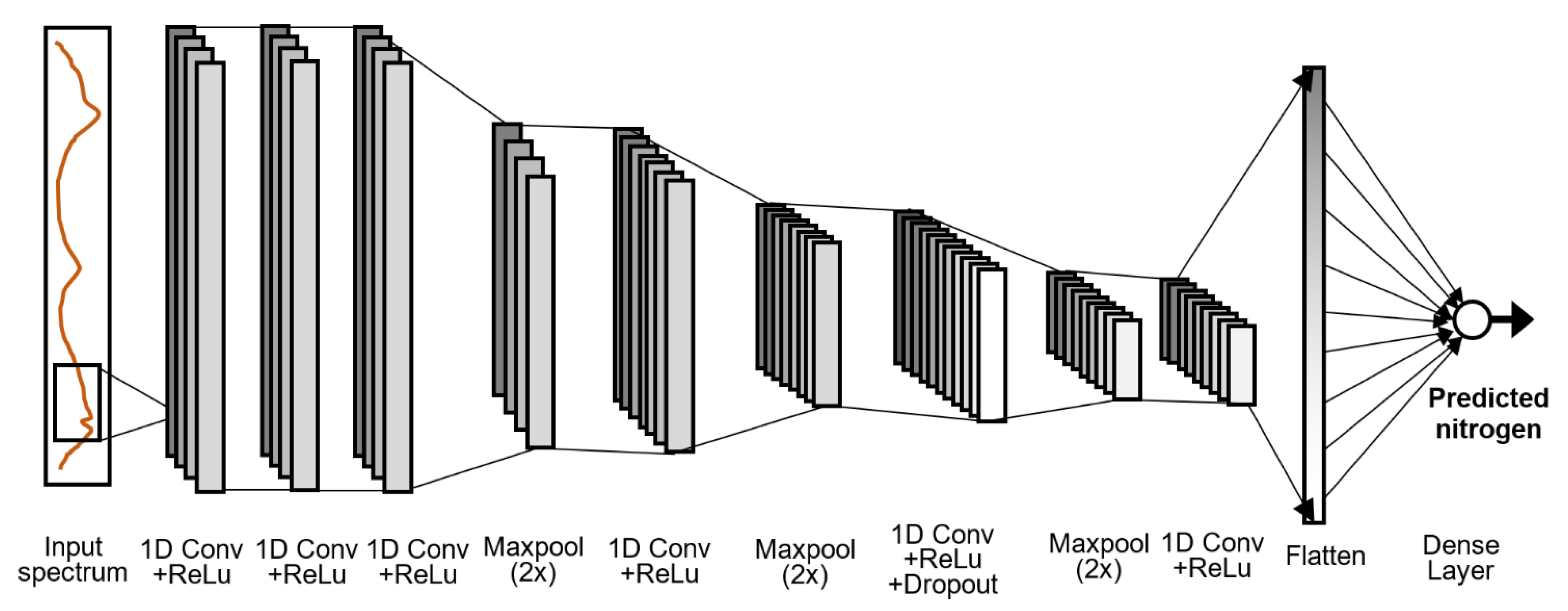
Consequently, the present paper describes a new one-dimensional (1D) convolutional neural network to estimate the nitrogen content of cucumber leaves. The innovation of this paper resides in the application of nitrogen overdose at 3 different levels, in order to investigate whether it is possible to detect nitrogen-rich cucumber on site and in real-time. Hyperspectral analysis of fruits and plants has been a very active area of research in the literature, and particularly in our research group, as previously seen. The main novelty of the present work resides in the proposal of a new 1D-CNN architecture with 12 layers. It contains six convolutional layers and three max-pooling layers, finishing with a dense layer, which produces the final estimation of nitrogen content. Another important element is the addition of a dropout layer that, by randomly removing some weights of the previous layer, avoids problems of overfitting.

2. Materials and Methods

The constituent stages of the proposed methodology for non-destructive estimation of nitrogen in cucumber plants can be seen in Figure 1. The steps of this methodology are described in detail in the following subsections.

2.1. Cultivation and Collection of Samples to Extract Spectral Data

According to the stages of the methodology in Figure 1, the first step is to prepare the samples with standard nitrogen fertilizer and with nitrogen over-dose. Hence, several seeds of cucumber of Super Arshiya’F1 variety were planted into 40 pots, and they were grown under laboratory conditions. All pots received the same inputs until the leaves grew; then the pots were divided into 4 groups of 10 pots. The first group with standard nitrogen was considered as the control treatment. A sample view of the pots in this category is shown in Figure 2. The second, third and fourth groups received nitrogen fertilizer overdoses by 30%, 60% and 90%, respectively.

After 24 h of applying the treatments, sample leaves were obtained from each group and their spectral signatures were extracted by a hyperspectral camera. The process for obtaining the samples of the dataset was as follows. First, 10 leaves were picked from each category, making a total of 40 cucumber leaves. For each leaf, the spectral images were captured, as described in Section 2.3, giving 327 images per leaf (one for each spectral band considered). This makes a total of 13,080 images. Then, the leaves were transferred to laboratory for the measurement of the nitrogen content by chemical analysis, as presented in Section 2.4. After manually analyzing the images, 10 patches were selected for each leaf in the 327 images, calculating the mean of each patch. Thus, 100 samples are available for each category, which consist of a tuple of 327 values, and the corresponding nitrogen content measured.

Although the process for obtaining this data is expensive (in terms of volume of images and laboratory analysis), the number of 100 samples per class is clearly insufficient for deep neural network analysis. For this reason, data augmentation was performed to obtain more synthetic samples. This was carried out by random weighted averaging of the real samples (i.e., computing a weighted average of two random tuples, and the same weighted average of the corresponding measured nitrogen content). Using this procedure, 900 synthetic samples per class were produced, totaling 1000 samples per class in the dataset (i.e., 4000 samples in the four classes).

2.2. Extraction of Spectral Data from Cucumber Leaves and Statistical Analysis

For the extraction of the spectral information of the cucumber leaves, a hyperspectral camera (Noor Iman Tajhiz Co., Kashan, Isfahan, Iran) at the range of 400–1100 nm was used. More specifically, 327 spectral images uniformly distributed in this range were obtained for each leaf, with a wavelength increment of 3.37 nm. To block out ambient light, the camera was located in an illumination chamber and exposed to two 10-watt tungsten halogen lamps (SLI-CAL, StellarNet Inc., Tampa, FL, USA). The spectral information in the Vis-NIR region was extracted and stored in a laptop. This laptop was a model DELL (DELL Co., Round Rock, TX, USA) with Intel Core i5, 2430 M at 2.40 GHz, 4 GB of RAM, and Windows 10. The original wavelengths were corrected by two methods: multiplicative scatter correction (MSC) in ParLeS software (Raphael Viscarra Rossel, Curtin University, Bentley, Australia), shown in Figure 3; and the smoothing operation by the Savitzky–Golay (SG) filtering algorithm [22].

Before creating the regression models, we checked whether the spectral information of the treatments are statistically significantly different or not. The spectral data of the four treatments (control, N_30%, N_60% and N_90%) were examined with two statistical tests: ANOVA test [23] and Duncan test [24]. The null hypothesis is that the mean values of the spectral wavelengths are the same for all the categories, and the alternative hypothesis is that they are different. That is, the input to the statistical tests are the 4000 samples, each of them a tuple of 327 values.

As it is well known, ANOVA test analyzes the null hypothesis for all the classes, while the Duncan test is a multiple comparison procedure between the pairs of classes. The results obtained for the ANOVA test are presented in

Table 1. ANOVA analysis for spectral data of the four categories of treatments: control, N_30%, N_60% and N_90%. The rows indicate the sum of squares between and within the classes, the number of degrees of freedom, the means of the squares between and within classes, the F-score (mean square between classes divided by mean square within classes), and the p-value of significance for an alpha of 0.05.

Category	Sum of Squares	Degrees of Freedom (df)	Mean Square	F-Score	Significance
Between Groups	8.15 × 1011	3	2.72 × 1011	5.69 × 103	0
Within Groups	1.91 × 1011	3996	4.78 × 107
Total	1.01 × 1012	3999

, and those corresponding to Duncan test are contained in

Table 2. Duncan test for spectral data related to the four categories of treatments, control, N_30%, N_60% and N_90%, at a significance level of 5%. Mean values of the classes are sorted in increasing order.

Treatment	Number	Subset for Alpha = 0.05
		Control	N30%	N60%	N90%
N60%	1000	9.2864 × 102
N30%	1000		1.7571 × 103
Control	1000			2.8540 × 103
N90%	1000				3.4779 × 104

.

The results of these tests indicate that the differences between the classes are statistically significant, both in the ANOVA test (Table 1) and in the Duncan test (Table 2), with a high level of significance. That is, the spectral wavelengths that reflect the presence of nitrogen are affected by the amount of nitrogen contained in the leaves. Thus, this justifies the development of different regression models for each class, since each of them produces distinct spectral features.

These tests do not prove any evidence about the linearity or non-linearity between the spectral information and the nitrogen content of the leaves. They only indicate that each class produces different spectral data. This is the reason for creating separate regression models. Although we could create a single regression model for all the classes, the statistical tests involve that, since the spectral data are different, more precise results can be obtained with individual models for each category.

2.3. Extraction of Nitrogen in Cucumber Leaves Using Laboratory Destructive Method

The Kjeldahl method was used to measure the total nitrogen content on the leaves. This method [25] includes three steps of digestion, distillation and titration. First, the leaves were dried in an oven and then powdered. Then, they are digested with sulfuric acid, so the nitrogen in the sample could be converted to ammonium sulfate. The nitrogen in ammonium sulfate was released in the form of ammonia and converted to ammonium borate with boric acid and titrated using 1% normal sulfuric acid; and then, the total nitrogen content of the sample can be obtained by calculating the consumed acid, as indicated in Equation (1):

$${\mathrm{N}}_{\mathrm{total}} (\%) = \frac{(vs-vb)}{md} \times {\mathrm{N}}_{\mathrm{H}2\mathrm{SO}4} \times {0.014}_{\mathrm{meqN}} \times 100$$

(1)

where:

vs: Volume consumed by the samples (mL),

vb: Volume consumed by the control treatment (mL),

N_H2SO4: Normality of sulfuric acid (equation/L),

md: Dry weight of the sample (g).

2.4. Non-Destructive Estimation of Nitrogen Using Convolutional Neural Networks

Deep learning (DL) is a category of machine learning algorithms that uses multiple layers to extract high-level features from raw input [26]. These kind of networks use multiple layers of information processing, especially nonlinear information, to perform the conversion or extraction of supervised or unsupervised features, generally for the purpose of pattern analysis or recognition, classification and clustering. Most deep learning methods use neural network structures, which is why DL models are often referred to as deep neural networks. Among them, convolutional neural networks (CNN) are one of the most popular techniques, since they do not require manual feature extraction. CNNs learn to recognize features from the samples using a large number of hidden layers. Each hidden layer increases the complexity of the features analyzed. Moreover, CNN networks do not change the structure of the input and pay attention to the connection between neighboring values.

Until now, most of the research has been conducted by known CNN structures such as AlexNet, VGG Net, ZF Net, GoogLeNet and fully convolutional networks (FCN) [27]. But in this paper, we proposed our personalized structure. In fact, it has been developed by examining several personalized structures by trial and error. Finally, the structure with the highest prediction rate was selected and proposed in this work.

More specifically, the proposed structure of the convolutional neural network used in this study is shown in Figure 4. The input vector of the algorithm contains the spectral data of a sample, and the output is the actual amount of nitrogen. Since, in our case, the input data is a one-dimensional (1D) spectrum, we used 1D convolutions. As shown, the architecture is similar to the well-known funnel design, where the size of the input is progressively reduced while the number of features increases. This is carried out by a succession of 1D convolutions and max-pooling layers. All the convolutions use the rectified linear (ReLu) activation function. The first part of the network contains 3 consecutive convolutional layers, then there are three steps of max-pooling and convolution. The second of these steps also includes a dropout layer, a method which is commonly used to avoid overfitting, since it randomly removes some weights in the previous convolutions, thus making the system more robust. The dropout rate was set to 0.1. Finally, the values of the last layer are flattened (producing 20,160 values) and a dense layer is responsible for producing the final estimation of nitrogen content.

It should be noted that among the 1000 samples in each category, 70% were used as the training data, and the remaining 30% as the test data, both sets disjoint. Moreover, the synthetic samples of the augmentation process were obtained after partitioning the real samples, so there is no mix of the training and test samples. The number of total epochs, batch-size, verbose and validation split were 200, 12, 1 and 0.1, respectively. The exact parameters of the proposed 1D-CNN are presented in

Table 3. Hyperparameters of the 1D convolutional neural network (1D-CNN) structure proposed in this paper for the estimation of nitrogen amount in cucumber leaves. Output shape refers to the size × number of features.

Layer (Type)	Output Shape	Kernel Size	Stride	Number of Parameters
Conv1d + ReLu	325 × 512	7	-	2048
Conv1d + ReLu	323 × 512	5	-	786,944
Conv1d + ReLu	321 × 512	5	-	786,944
Max pooling	160 × 256		2	-
Conv1d + ReLu	156 × 256	3	-	196,864
Max pooling	78 × 128		2	-
Conv1d + ReLu	76 × 128	3	-	49,280
Dropout (0.1)			-	0
Max pooling	38 × 128		2	-
Conv1d + ReLu	36 × 64	3	-	12,352
Flatten	20160		-	0
Dense + Relu	1		-	20,161

Total params: 2,031,233; trainable params: 2,031,233; non-trainable params: 0.

.

2.5. Evaluation of the Performance of the Methods for the Estimation of Nitrogen in Cucumber

To evaluate the performance of the prediction model, the statistical parameters including score-variance (Var-score) [28], max error (MaxE) [29], mean absolute error (MAE) [30], mean squared error (MSE) [31], coefficient of determination (R²) [32], median absolute error (MedAE) [33] and mean squared logarithmic error (MSLE) [34] were used. Consider that the expected outputs for a given variable are Y_i, for i ranging in the number of samples, n, and consider that X_i represents the corresponding estimated values. Then, the proposed performance measures are given in the following equations:

$$\mathrm{MSE}=\frac{1}{n}\sum _{s=1}^n{(X_s-Y_s)}^2$$

(2)

$$\mathrm{MedAE}=\mathrm{median}\left\{{\sum }_{s=1}^n\mathrm{\right|}{X}_s-Y_s\mathrm{\left|}\right\}$$

(3)

$$\mathrm{MAE}=\frac{1}{n}{\sum }_{s=1}^n|X_s-Y_s|$$

(4)

$$\mathrm{MaxE}=\max \left\{{\sum }_{s=1}^n\mathrm{\right|}{X}_s-Y_s\mathrm{\left|}\right\}$$

(5)

$${\mathrm{R}}^2=1-\left\{\frac{{\sum }_{s=1}^n{(X_s-Y_s)}^2}{{\sum }_{s=1}^n{(X_s-X_m)}^2}\right\}$$

(6)

$$\mathrm{MSLE}=\frac{1}{n}{\sum }_{s=1}^n\log {(X_s-Y_s)}^2$$

(7)

$$\mathrm{Var}-\mathrm{score}=\mathrm{variance}\left(X_s\right)/\mathrm{variance}\left(Y_s\right)$$

(8)

$$X_m=\frac{1}{n}{\sum }_{s=1}^n{X}_s$$

(9)

3. Results

In the following subsections, the results achieved by the regression models created for each treatment are presented. All of them are 1D-CNN networks that are specifically trained for the corresponding class.

3.1. Prediction Model for the Category with Excess of Nitrogen by 30%

Preprocessing is needed to reduce the noise in the spectral information, so different algorithms of correction and smoothing filters were examined.

Table 4. Evaluation of the prediction model for the category with excess of nitrogen by 30%. Filtering algorithms: MSC: multiplicative scatter correction; SG: Savitzky–Golay filter. MAE: mean absolute error; MSE: mean squared error; MSLE: mean squared logarithmic error; MedAE: median absolute error; MaxE: max error; R²: coefficient of determination; Var-score: variance score.

Algorithm	MAE	MSE	MSLE	MedAE	MaxE	R2	Var-Score
MSC + SG	0.017	0.0005	0.00002	0.014	0.086	0.962	0.974
MSC	0.022	0.0011	0.00009	0.015	0.084	0.951	0.971
SG	0.02	0.0009	0.00005	0.013	0.072	0.958	0.972
No filter	0.027	0.0016	0.00012	0.018	0.092	0.941	0.967

contains the results of evaluating the performance of the prediction model for the category with nitrogen overdose by 30%, using different correction and smoothing algorithms. As described in Section 2, these filters are: multiplicative scatter correction (MSC), smoothing by the Savitzky–Golay (SG) filter.

All the error measures can be observed to be very low, while R² is close to 1, indicating that the model is able to accurately estimate nitrogen content in this class. Figure 5 shows the regression plot between the amount of nitrogen measured by the Kjeldahl method, and the mean estimated nitrogen for 300 test data. The proximity of these two values indicates the ability of the proposed model. Figure 6 shows the train loss and validation loss diagrams for the nitrogen content during the training process. The maximum number of epochs was set to 200. In addition, we added a condition to early stop training if over-fitting is detected (i.e., when training loss decreases but validation loss increases). As shown in Figure 6, it can be seen that after 17 epochs training stopped and the loss rate is very close to 0%.

3.2. Prediction Model for the Category with Excess of Nitrogen by 60%

The statistical criteria for evaluating the performance of the prediction model are given in

Table 5. Evaluation of the prediction model for the category with excess of nitrogen by 60%. Filtering algorithms: MSC: multiplicative scatter correction; SG: Savitzky–Golay filter. MAE: mean absolute error; MSE: mean squared error; MSLE: mean squared logarithmic error; MedAE: median absolute error; MaxE: max error; R²: coefficient of determination; Var-score: variance score.

Algorithm	MAE	MSE	MSLE	MedAE	MaxE	R2	Var-Score
MSC + SG	0.014	0.0003	0.00001	0.014	0.091	0.968	0.984
MSC	0.017	0.0007	0.00006	0.017	0.094	0.953	0.972
SG	0.015	0.0005	0.00003	0.016	0.092	0.962	0.976
No filter	0.019	0.0012	0.00009	0.019	0.096	0.938	0.963

for the category N_60%. Again, it can be seen that the error measures are very close to 0, so the proposed model was successful for the prediction of nitrogen in the treatment of 60% overdose. Moreover, the results indicate the positive effect of the filtering algorithms.

Figure 7 shows the regression plot of the measured and the estimated nitrogen content for this category, for the 300 test samples used. These two values are close to each other, indicating the ability of the proposed model. Figure 8 illustrates that after 43 epochs, the training process stopped due to over fitting. At that step, the training achieved the optimal result.

3.3. Prediction Model for the Category with Excess of Nitrogen by 90%

Regarding the treatment of 90% nitrogen overdose, the statistical criteria for evaluating the performance of the prediction model are given in

Table 6. Evaluation of the prediction model for the category with excess of nitrogen by 90%. Filtering algorithms: MSC: multiplicative scatter correction; SG: Savitzky–Golay filter. MAE: mean absolute error; MSE: mean squared error; MSLE: mean squared logarithmic error; MedAE: median absolute error; MaxE: max error; R²: coefficient of determination; Var-score: variance score.

Algorithm	MAE	MSE	MSLE	MedAE	MaxE	R2	Var-Score
MSC + SG	0.023	0.0007	0.00001	0.022	0.054	0.967	0.983
MSC	0.027	0.0009	0.00004	0.026	0.058	0.953	0.978
SG	0.025	0.0008	0.00002	0.023	0.055	0.961	0.981
No filter	0.028	0.0013	0.00006	0.029	0.061	0.949	0.969

, indicating the mean error measures and the variance score and coefficient of determination. Again, the measures achieved are very positive and indicate a great accuracy of the proposed model.

Figure 9 depicts the regression plot of the measured amount of nitrogen and the mean estimated values for 300 test data in this treatment. As indicated in Table 6, the prediction is done with a correlation coefficient of 0.967.

Figure 10 shows that after 41 epochs, the training process stopped due to the detection of the over fitting criterion. Both the train and validation loss present a similar behavior. Initially, there is a fast reduction during the first 5–6 epochs of training. Then, there is a more smooth and progressive reduction of both loss values, approximately until epoch 25. Finally, the system stabilizes and the process is stopped before the validation loss begins to increase (which would mean that overfitting is starting).

4. Discussion

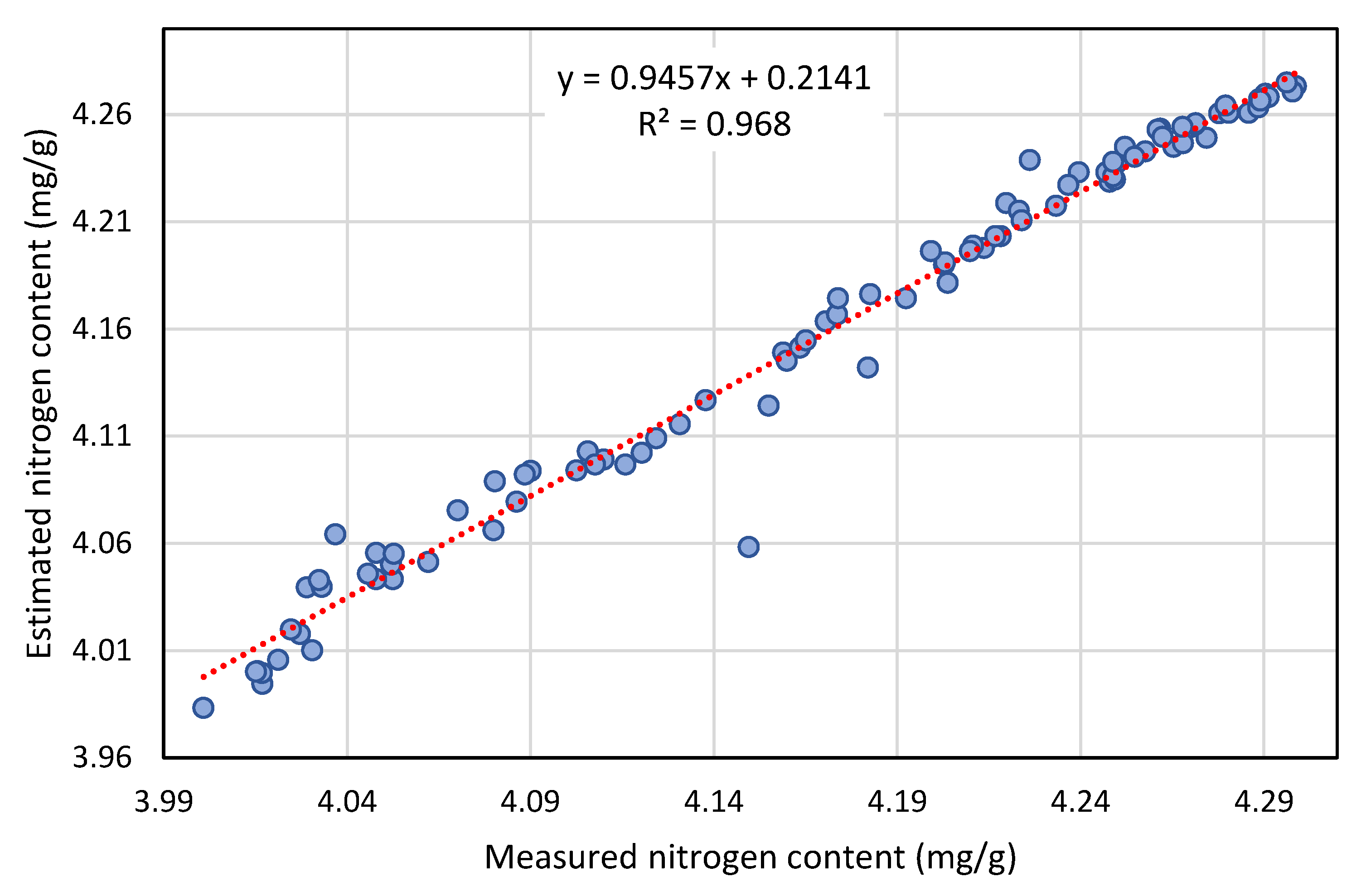
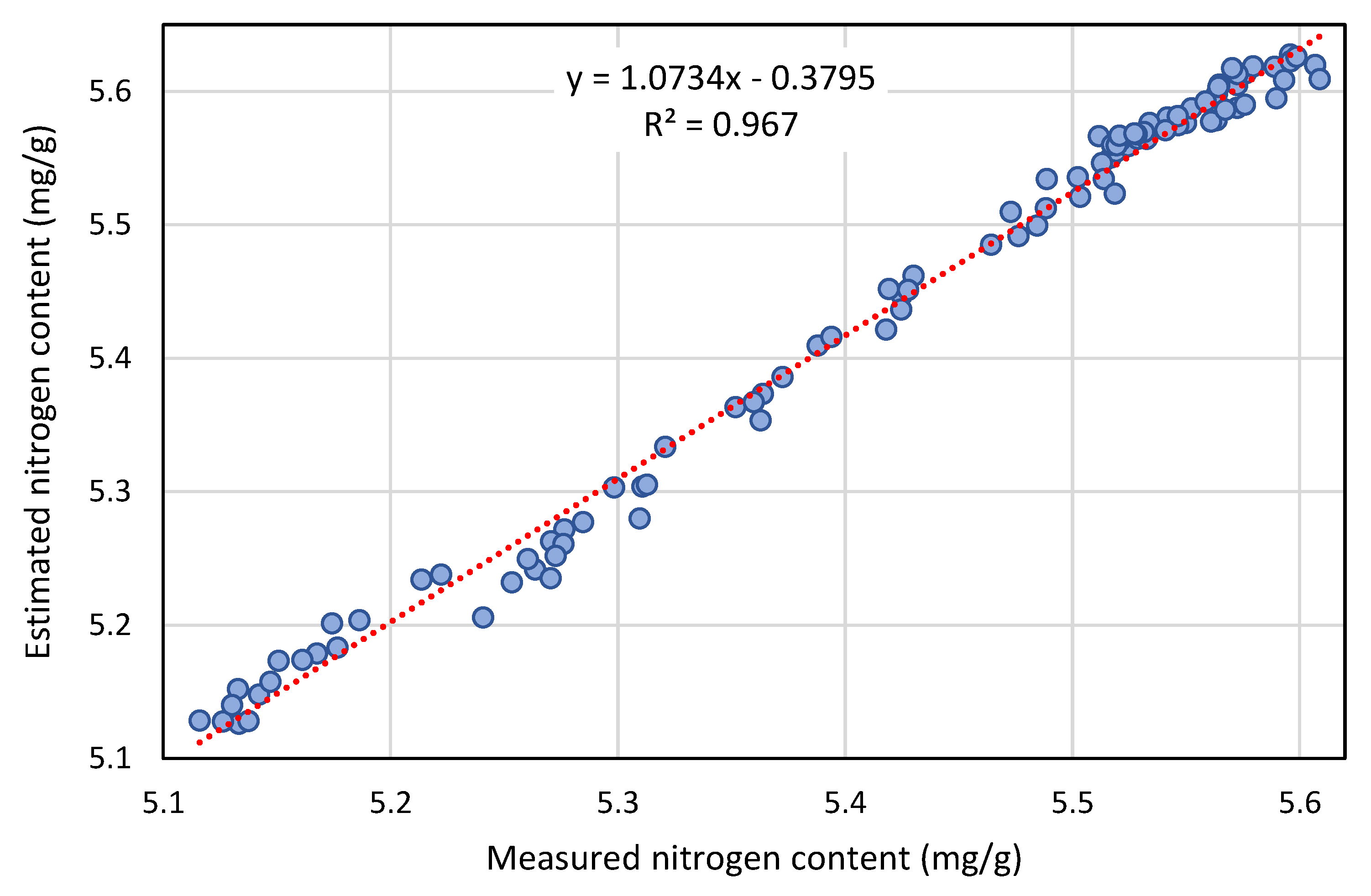
In general, the results presented in the previous section prove that the nitrogen content of cucumber leaves can be estimated with a high accuracy using hyperspectral information in the Vis-NIR range and the proposed 1D-CNN regression models. The obtained mean errors are always below 1% with respect to the expected values for all the treatments. For example, in the N_30% class, the mean absolute error (MAE) is only 0.017 mg/g, while the nitrogen content ranges from 3–3.4 mg/g; this would represent a 0.56% relative error. The relative MAE for the N_60% and N_90% classes are 0.35% and 0.45%, respectively. This means that the proposed approach can be effectively used for the estimation of nitrogen in the leaves from the early stages, since the error is very small even for the 30% class.

This positive result can also be argued even for the worst cases of error, i.e., considering the maximum errors, MaxE. This error is 0.086 mg/g for N_30% class and 0.091 mg/g for N_60% class, which represent relative errors below 3%. In the N_90% class, this worst case has a very low error of 0.054 mg/g. Therefore, we can conclude that the method does not present cases of extremely high error. This is evidence of the robustness of the proposed approach against the most difficult cases.

Regarding the preprocessing techniques applied in the paper, MSC and SG, both steps prove to have positive effects on the obtained results. Observe that MSC is a scatter correction filter of the spectra, while SG is a smoothing operator. In all the treatments, the worst results are given by not applying any filter, which is evident for all the performance measures. For example, in the 60% class, the MSE is 0.0003 mg/g with the proposed filters, MSC + SG, while it rises to 0.0012 mg/g with no preprocessing filter. If we should select only one filter, the smoothing step, SG, is the method that offers the best results by itself in terms of the error. For example, in the 90% class, the MAE without any filter is 0.028 mg/g; with SG it descends to 0.025, but with MSG it is 0.027. This indicates that smoothing is more beneficial than scatter correction. This is also repeated for the determination coefficient, R², which is consistently higher for SG. Moreover, the improvement from applying MSC + SG with respect to applying only SG is very reduced in most cases, with a small positive effect in the error measures.

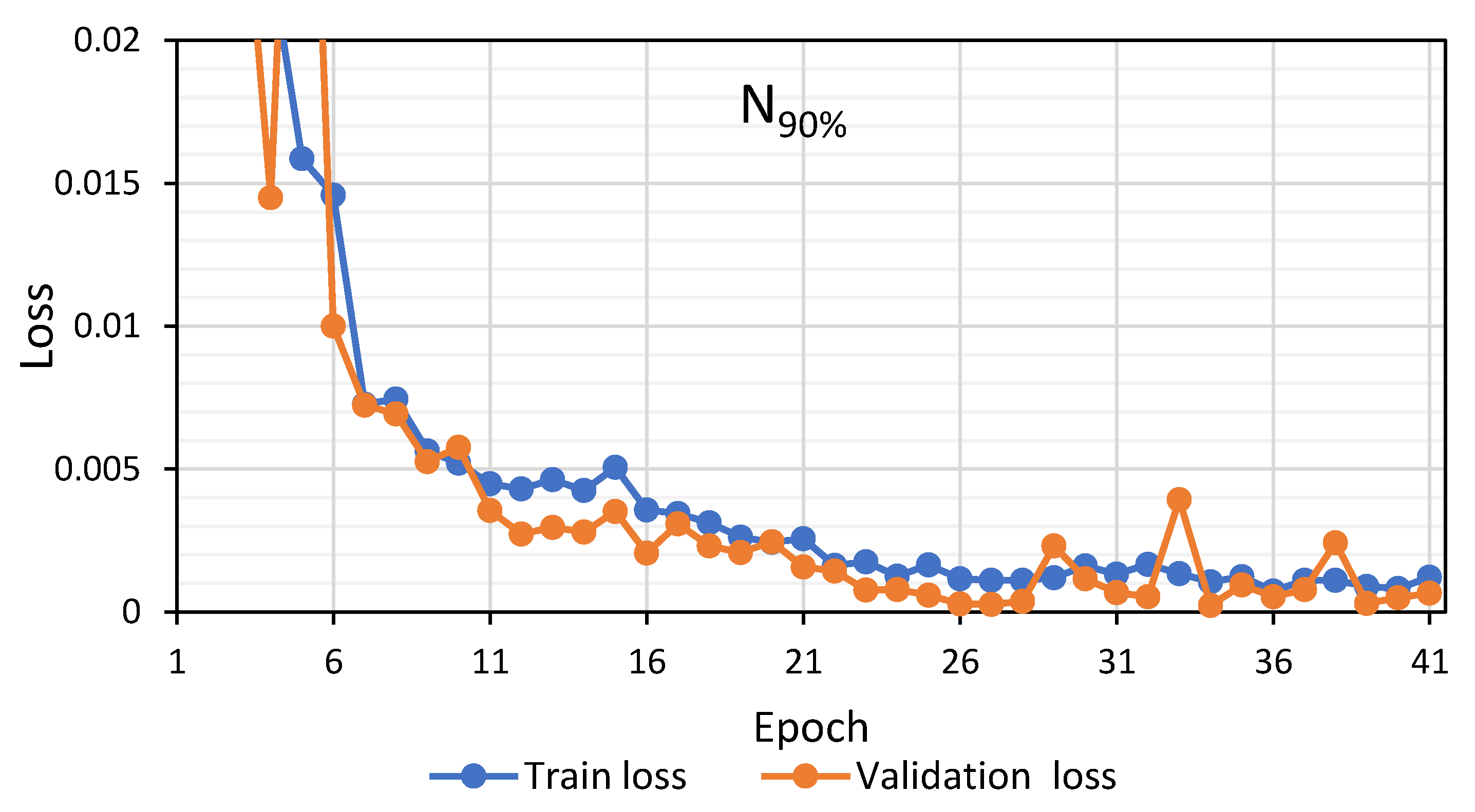
Analyzing the evolution of the loss curves in Figure 6, Figure 8 and Figure 10, it can be seen that the proposed 1D-CNN has a very fast convergence for all the treatments. A fast reduction of the loss values is produced in the first five epochs. Then, the system enters in a gradual convergence phase, which is stopped before it could incur in over-fitting. No model required more than 43 epochs, making them relatively fast to be trained. The loss curves also indicate that the training process does not incur in over-fitting, which would appear as a reduction of the train loss and an increment in the validation loss.

Finally,

Table 7. Comparison the coefficient of determination, R², of the proposed 1D-CNN method with other existing methods.

Methods	Product	Method	Prediction	R2
Proposed method for N30%	Cucumber	1D-CNN	Excess nitrogen	0.962
Proposed method for N60%	Cucumber	1D-CNN	Excess nitrogen	0.968
Proposed method for N90%	Cucumber	1D-CNN	Excess nitrogen	0.967
(Pourdarbani et al. [35])	Tomato	PLSR	Nitrogen content	0.702
(Pourdarbani et al. [35])	Tomato	ANN-DE	Nitrogen content	0.747
(Pourdarbani et al. [35])	Tomato	CNN	Nitrogen content	0.766
(Torkashvand et al. [22])	Kiwifruit	ANN	Nutrient content	0.85
(Huang et al. [36])	Tomato	ANN	SSC	0.81
(Ghosal et al. [37])	Soybean	CNN	K & Fe	0.94

presents a comparison of the results achieved by the proposed 1D-CNN models, compared with the results of other researchers for the non-destructive estimation of different properties of fruits, using R² criterion. Although these works have been selected among the most similar to our proposed method, this comparison has to be considered in context, since they refer to different types of fruits, different datasets, and distinct types of regression models. We have also included the results of a previous study from our group that deals with the estimation of nitrogen in tomato leaves, using different types of classifiers [35]. Overall, the results of the present study showed that using 1D-CNN based on spectral data, it is possible to estimate the excess nitrogen more accurately, achieving results that are in the state of the art.

Comparing the obtained results with the accuracy reported in [35], it can be seen that the R² are significantly better. These methods include partial least squares regression (PLSR) which is a statistical-based method, and hybrid approach of classical neural networks and the differential evolution algorithm (ANN-DE), and a method similar to the proposed in this paper using convolutional neural networks (CNN). In all of them, a unique model is trained for all the nitrogen categories, producing poor regression results always below 0.8 in R². Instead, the approach of creating separate models for each class is able to produce better results above 0.96. In fact, the approach of training different models for the classes was also analyzed in [35], although the R² achieved ranged from 0.925 to 0.968.

On the other hand, a weak point of the proposed method is that it requires a previous classification of the leaf samples in the corresponding treatment class. Given a new unknown sample, there are three different models that could be applied on it. Thus, a classifier would be required to obtain the class before applying the regression network. This classification problem has been previously studied in our group, finding that it is possible to achieve it with a classification accuracy above 96% [10]. This would complete a system based on two steps: first, classification of the sample; and then, regression of the nitrogen content using the specific model. The results discussed in this section indicate that this approach is able to produce better results than training a single regression model for all the classes.

5. Conclusions

Scientific management of production and consumption of fertilizers is necessary to achieve sustainable agriculture, and to improve food health by improving the optimal use of them, especially nitrogen-based fertilizers. In this paper, we have presented a new methodology for fast and accurate estimation of nitrogen content in cucumber leaves using spectroscopy analysis and convolutional neural networks (CNN).

Currently, CNNs are one of the most popular methods of machine learning, since they do not require manual feature extraction. Instead, automatic feature extraction makes deep learning models very accurate for computer vision tasks, such as regression models. Therefore, we have presented a new structure of one-dimensional CNN (1D-CNN) to estimate nitrogen content. Different levels of nitrogen fertilizer overdose by 30%, 60% and 90% were added to the cucumbers, and then prediction models were trained for each treatment. The experimental results have shown that the proposed 1D-CNN is able to estimate very accurately the nitrogen content even in the early stages, achieving, for example, for the 30% treatment, a maximum error of 0.086 mg/g and an R² of 0.962. For the 60% and 90% classes, the R² are 0.968 and 0.967, respectively. The experiments also showed that the applied preprocessing filters, multiplicative scatter correction, Savitzky–Golay, had a positive effect on the accuracy. Thus, this approach can be used to create a fast and non-destructive method to prevent excessive use of fertilizers.

References

1. Balafoutis, A.; Beck, B.; Fountas, S.; Vangeyte, J.; Van Der Wal, T.; Soto, I.; Gómez-Barbero, M.; Barnes, A.; Eory, V. Precision Agriculture Technologies Positively Contributing to GHG Emissions Mitigation, Farm Productivity and Economics. Sustainability 2017, 9, 1339. [Google Scholar] [CrossRef] [Green Version]
2. Agarwal, M.; Gupta, S.K.; Biswas, K. Development of Efficient CNN model for Tomato crop disease identification. Sustain. Comput. Inform. Syst. 2020, 28, 100407. [Google Scholar] [CrossRef]
3. Sabzi, S.; Pourdarbani, R.; Kalantari, D.; Panagopoulos, T. Designing a Fruit Identification Algorithm in Orchard Conditions to Develop Robots Using Video Processing and Majority Voting Based on Hybrid Artificial Neural Network. Appl. Sci. 2020, 10, 383. [Google Scholar] [CrossRef] [Green Version]
4. Fatchurrahman, D.; Amodio, M.L.; de Chiara, M.L.V.; Chaudhry, M.M.A.; Colelli, G. Early discrimination of mature-and immature-green tomatoes (Solanum lycopersicum L.) using fluorescence imaging method. Postharvest Biol. Technol. 2020, 169, 111287. [Google Scholar] [CrossRef]
5. Martínez-Dalmau, J.; Berbel, J.; Ordóñez-Fernández, R. Nitrogen Fertilization. A Review of the Risks Associated with the Inefficiency of Its Use and Policy Responses. Sustainability 2021, 13, 5625. [Google Scholar] [CrossRef]
6. Maynard, D.N.; Barker, A.V.; Minotti, P.L.; Peck, N.H. Nitrate Accumulation in Vegetables. In Advances in Agronomy; Brady, N.C., Ed.; Academic Press: Cambridge, CA, USA, 1976; Volume 28, pp. 71–118. [Google Scholar]
7. Renseigné, N.; Umar, S.; Iqbal, M. Nitrate accumulation in plants, factors affecting the process, and human health implications. A review. Agron. Sustain. Dev. 2007, 27, 45–57. [Google Scholar]
8. Dezordi, L.R.; Aquino, L.A.D.; Aquino, R.F.B.D.A.; Clemente, J.M.; Assunção, N.S. Diagnostic methods to assess the nutritional status of the carrot crop. Rev. Bras. Ciência Solo 2016, 40. [Google Scholar] [CrossRef]
9. Nandhini, S.; Suganya, R.; Nandhana, K.; Varsha, S.; Deivalakshmi, S.; Thangavel, S.K. Automatic Detection of Leaf Disease Using CNN Algorithm. In Machine Learning for Predictive Analysis; Lecture Notes in Networks and Systems; Springer: Singapore, 2021. [Google Scholar] [CrossRef]
10. Sabzi, S.; Pourdarbani, R.; Rohban, M.; García-Mateos, G.; Paliwal, J.; Molina-Martínez, J. Early Detection of Excess Nitrogen Consumption in Cucumber Plants Using Hyperspectral Imaging Based on Hybrid Neural Networks and the Imperialist Competitive Algorithm. Agronomy 2021, 11, 575. [Google Scholar] [CrossRef]
11. Wang, Z.; Zheng, C.; Ma, C.; Ma, B.; Wang, J.; Zhou, B.; Xia, T. Comparative analysis of chemical constituents and antioxidant activity in tea-leaves microbial fermentation of seven tea-derived fungi from ripened Pu-erh tea. LWT 2021, 142, 111006. [Google Scholar] [CrossRef]
12. Hubel, D.H.; Wiesel, T.N. Receptive fields, binocular interaction and functional architecture in the cat’s visual cortex. J. Physiol. 1962, 160, 106–154. [Google Scholar] [CrossRef]
13. Zhu, L.; Spachos, P.; Pensini, E.; Plataniotis, K.N. Deep learning and machine vision for food processing: A survey. Curr. Res. Food Sci. 2021, 4, 233–249. [Google Scholar] [CrossRef] [PubMed]
14. Watchareeruetai, U.; Noinongyao, P.; Wattanapaiboonsuk, C.; Khantiviriya, P.; Duangsrisai, S. Identification of Plant Nutrient Deficiencies Using Convolutional Neural Networks. In Proceedings of the 2018 International Electrical Engineering Congress (iEECON), Krabi, Thailand, 7–9 March 2018; pp. 1–4. [Google Scholar]
15. Espejo-Garcia, B.; Mylonas, N.; Athanasakos, L.; Fountas, S. Improving weeds identification with a repository of agricultural pre-trained deep neural networks. Comput. Electron. Agric. 2020, 175, 105593. [Google Scholar] [CrossRef]
16. Sharma, N.; Sharma, R.; Jindal, N. Machine Learning and Deep Learning Applications-A Vision. Global Transitions Proc. 2021, 2, 24–28. [Google Scholar] [CrossRef]
17. Liu, Q.; Zhou, F.; Hang, R.; Yuan, X. Bidirectional-Convolutional LSTM Based Spectral-Spatial Feature Learning for Hyperspectral Image Classification. Remote Sens. 2017, 9, 1330. [Google Scholar] [CrossRef] [Green Version]
18. Tian, X.; Li, J.; Yi, S.; Jin, G.; Qiu, X.; Li, Y. Nondestructive determining the soluble solids content of citrus using near infrared transmittance technology combined with the variable selection algorithm. Artif. Intell. Agric. 2020, 4, 48–57. [Google Scholar] [CrossRef]
19. Cai, H.-T.; Liu, J.; Chen, J.-Y.; Zhou, K.-H.; Pi, J.; Xia, L.-R. Soil nutrient information extraction model based on transfer learning and near infrared spectroscopy. Alex. Eng. J. 2021, 60, 2741–2746. [Google Scholar] [CrossRef]
20. Wittwer, S.H.; Honma, S. Greenhouse Tomatoes, Lettuce and Cucumbers; Michigan State University Press: East Lansing, MI, USA, 1979. [Google Scholar]
21. Mehta, D.; Choudhury, T.; Sehgal, S.; Sarkar, T. Fruit Quality Analysis using modern Computer Vision Methodologies. In Proceedings of the 2021 IEEE Madras Section Conference (MASCON), Chennai, India, 27–28 August 2021; pp. 1–6. [Google Scholar]
22. Torkashvand, A.M.; Ahmadi, A.; Nikravesh, N.L. Prediction of kiwifruit firmness using fruit mineral nutrient concentration by artificial neural network (ANN) and multiple linear regressions (MLR). J. Integr. Agric. 2017, 16, 1634–1644. [Google Scholar] [CrossRef] [Green Version]
23. Miller, R.G. Beyond ANOVA: Basics of Applied Statistics; Chapman & Hall: Boca Raton, FL, USA, 1997. [Google Scholar]
24. Duncan, D.B. Multiple Range and Multiple F Tests. Biometrics 1955, 11, 1–42. [Google Scholar] [CrossRef]
25. Kjeldahl, J. Neue Methode zur Bestimmung des Stickstoffs in organischen Körpern (New method for the determination of nitrogen in organic substances). Z. Anal. Chem. 1883, 22, 366–383. [Google Scholar] [CrossRef] [Green Version]
26. LeCun, Y.; Bengio, Y.; Hinton, G. Deep learning. Nature 2015, 521, 436–444. [Google Scholar] [CrossRef] [PubMed]
27. Liu, W.; Wang, Z.; Liu, X.; Zeng, N.; Liu, Y.; Alsaadi, F.E. A survey of deep neural network architectures and their applications. Neurocomputing 2016, 234, 11–26. [Google Scholar] [CrossRef]
28. Kristof, W. Estimation of true score and error variance for tests under various equivalence assumptions. Psychometrika 1969, 34, 489–507. [Google Scholar] [CrossRef]
29. Douglas, F.; Yang, C.; Malcolm, S. The Maximum-Error Test. J. Astronaut. Sci. 2020, 55, 259–270. [Google Scholar]
30. Sabzi, S.; Pourdarbani, R.; Arribas, J.I. A Computer Vision System for the Automatic Classification of Five Varieties of Tree Leaf Images. Computers 2020, 9, 6. [Google Scholar] [CrossRef] [Green Version]
31. Pourdarbani, R.; Sabzi, S.; Kalantari, D.; Arribas, J.I. Non-destructive visible and short-wave near-infrared spectroscopic data estimation of various physicochemical properties of Fuji apple (Malus pumila) fruits at different maturation stages. Chemom. Intell. Lab. Syst. 2020, 206, 104147. [Google Scholar] [CrossRef]
32. Pourdarbani, R.; Sabzi, S.; Kalantari, D.; Paliwal, J.; Benmouna, B.; García-Mateos, G.; Molina-Martínez, J.M. Estimation of different ripening stages of Fuji apples using image processing and spectroscopy based on the majority voting method. Comput. Electron. Agric. 2020, 176, 105643. [Google Scholar] [CrossRef]
33. Wang, W.; Lu, Y. Analysis of the mean absolute error (MAE) and the root mean square error (RMSE) in assessing rounding model. In IOP Conference Series: Materials Science and Engineering; IOP Publishing: Bristol, UK, 2018; Volume 324, p. 012049. [Google Scholar]
34. Jeong, J.H.; Woo, J.H.; Park, J. Machine Learning Methodology for Management of Shipbuilding Master Data. Int. J. Nav. Arch. Ocean Eng. 2020, 12, 428–439. [Google Scholar] [CrossRef]
35. Pourdarbani, R.; Sabzi, S.; Rohban, M.; Garcia-Mateos, G.; Arribas, J. Nondestructive nitrogen content estimation in tomato (Solanum lycopersicum L) plant leaves by Vis-NIR hyperspectral imaging and regression data models. Appl. Opt. 2021, 60, 9560–9569. [Google Scholar] [CrossRef]
36. Huang, Y.; Lu, R.; Chen, K. Assessment of tomato soluble solids content and pH by spatially-resolved and conventional Vis/NIR spectroscopy. J. Food Eng. 2018, 236, 19–28. [Google Scholar] [CrossRef]
37. Ghosal, S.; Blystone, D.; Singh, A.K.; Ganapathysubramanian, B.; Singh, A.; Sarkar, S. An explainable deep machine vision framework for plant stress phenotyping. Proc. Natl. Acad. Sci. USA 2018, 115, 4613–4618. [Google Scholar] [CrossRef] [Green Version]
Figure 1. Main stages of the non-destructive estimation of nitrogen in cucumber plants.
Applsci 11 11853 g001
Figure 2. Cucumber pots prepared for data collection.
Applsci 11 11853 g002
Figure 3. Sample of the application of spectral preprocessing using ParLeS software.
Applsci 11 11853 g003
Figure 4. Architecture of the proposed 1D convolutional neural network for the estimation of nitrogen content.
Applsci 11 11853 g004
Figure 5. Regression plot of the measured and estimated nitrogen content for category N30%.
Applsci 11 11853 g005
Figure 6. Train loss and validation loss diagram for category N30%.
Applsci 11 11853 g006
Figure 7. Regression plot of the measured and estimated nitrogen content for category N60%.
Applsci 11 11853 g007
Figure 8. Train loss and validation loss diagram for category N60%.
Applsci 11 11853 g008
Figure 9. Regression plot of the measured and estimated nitrogen content for category N90%.
Applsci 11 11853 g009
Figure 10. Train loss and validation loss diagram for category N90%.
Applsci 11 11853 g010