Article

Field Data Forecasting Using LSTM and Bi-LSTM Approaches

1
DISP Laboratory, University Lumiere Lyon 2, 69500 Bron, France
2
CAMT, Chiang Mai University, Chiang Mai 50200, Thailand
3
Joaan Bin Jassim Academy for Defence Studies, Doha P.O. Box 24939, Qatar
4
CSE, College of Engineering, Qatar University, Doha 2713, Qatar
*
Author to whom correspondence should be addressed.
Appl. Sci. 2021, 11(24), 11820; https://doi.org/10.3390/app112411820
Submission received: 22 October 2021 / Revised: 22 November 2021 / Accepted: 26 November 2021 / Published: 13 December 2021

Abstract

:
Water, an essential resource for crop production, is becoming increasingly scarce, while cropland continues to expand due to the world’s population growth. Proper irrigation scheduling has been shown to help farmers improve crop yield and quality, resulting in more sustainable water consumption. Soil Moisture (SM), which indicates the amount of water in the soil, is one of the most important crop irrigation parameters. In terms of water usage optimization and crop yield, estimating future soil moisture (forecasting) is an essentially valuable task for crop irrigation. As a result, farmers can base crop irrigation decisions on this parameter. Sensors can be used to estimate this value in real time, which may assist farmers in deciding whether or not to irrigate. The soil moisture value provided by the sensors, on the other hand, is instantaneous and cannot be used to directly compute irrigation parameters such as the best timing or the required water quantity to irrigate. The soil moisture value can, in fact, vary greatly depending on factors such as humidity, weather, and time. Using machine learning methods, these parameters can be used to predict soil moisture levels in the near future. This paper proposes a new Long-Short Term Memory (LSTM)-based model to forecast soil moisture values in the future based on parameters collected from various sensors as a potential solution. To train and validate this model, a real-world dataset containing a set of parameters related to weather forecasting, soil moisture, and other related parameters was collected using smart sensors installed in a greenhouse in Chiang Mai province, Thailand. Preliminary results show that our LSTM-based model performs well in predicting soil moisture with a 0.72% RMSE error and a 0.52% cross-validation error (LSTM), and our Bi-LSTM model with a 0.76% RMSE error and a 0.57% cross-validation error. In the future, we aim to test and validate this model on other similar datasets.

1. Introduction

‘Water’ is one of the most important resources required for crop production. In different stages of crops life cycles, they require different amounts of water. Water influences, among other things, respiration, photosynthesis, mineral nutrient translocation, absorption, mineral nutrient utilization, and cell division. Water scarcity has a huge impact on crop quality and yield. As a result, water has an impact on nutrient availability, operation timing, and other factors, in addition to having a direct impact on crop production [1]. As a result, crops require watering in order to grow and develop. Crop watering, also known as ‘irrigation,’ is a method used to help crops grow as an alternative to rain-fed farming. Canals, sprinklers, pipes, sprays, drips, pumps, and other man-made devices provide irrigation [2,3].
According to the report of AQUASTAT [4], water withdrawal ratios of the Earth’s freshwater are 70% in the agricultural sector for crop irrigation, 11% in municipal, and 19% in industrial, indicating that agriculture is by far the largest consumer of the Earth’s available freshwater. Meanwhile, freshwater accounts for only 0.5% of the world’s water, with seawater accounting for the majority (97%) and frozen water accounting for the remaining 2.5% [5]. Irrigation needs are expected to increase agriculture’s global water demand by 15% by 2050 [6]. Currently, artificially irrigated areas produce approximately 40% of the world’s food [7]. Agriculture’s water needs, on the other hand, already compete with people’s and the environment’s daily needs, particularly in areas where irrigation is required, threatening ecosystem survival. According to an OECD report, agriculture production is heavily reliant on water, and water threats are becoming more prevalent as agricultural regions around the world have faced water issues in recent years [7]. Furthermore, agriculture is both the primary user of water for agricultural production and the primary polluter of water due to the use of chemical pesticides and fertilizers. Moreover, in the coming years, climate change will have a significant and uncertain impact on water supply [7]. As a result, agricultural water management must be improved in order to make agriculture more sustainable, contributing to global food and water security.
Irrigation scheduling is the process by which irrigators determine and manage crop watering frequency and duration. Farmers benefit from irrigation scheduling by increasing crop yield and quality while reducing water loss due to deep precipitation and runoff, lowering pumping costs, increasing water efficiency, and ensuring long-term sustainable water usage. Four parameters are required to successfully schedule irrigation: soil moisture content, soil water holding capacity, soil texture, and crop water use at various growing stages [8]. It is also necessary to consider the irrigation system’s capacity. During the growing season, different crop types consume varying amounts of water. For example, canola consumes water at a rate of seven mm/day during pod fill, but consumes water at only two mm/day during the rosette stage. Peas, for example, can consume water at a maximum of six mm/day and no more than two mm/day during pod development [9,10]. In this paper, we focus on soil-based methods because we are predicting water requirements before drought stress occurs. Based on soil moisture measurements, the soil-based approach calculates the amount of water currently available to the crop. Smart irrigation technologies are now being used to assist irrigators with on-site field moisture measurement in order to predict soil moisture values for optimal water usage [10,11]. This prediction will be used to estimate and schedule irrigation in order to improve irrigation controls by tracking moisture-related conditions on the field and performing watering at optimal levels automatically [12]. The smart irrigation technology that this paper focuses on is soil moisture-based smart irrigation. This technology employs sensors to determine the actual moisture content of the soil. It adjusts the time of water irrigation based on this information. However, one of soil moisture sensors current limitations is their inability to report on or represent the entire farm. Farmers must install a large number of soil moisture sensors in each area of the farm to monitor soil moisture, which raises their costs. As a result, soil moisture value forecasting is a low-cost but promising software-based alternative that requires fewer sensors and can produce accurate predictions when given the right set of input data.
There are significant advantages to combining technological advances and farmer experience, such as improved crop quality and yield, as well as water savings through effective irrigation mechanisms. Our ultimate goal is to develop an automated water irrigation management system that uses a variety of technologies and tools to aid farmers’ decision-making and automate the water management process. The Internet of Things (IoT) makes use of various types of sensors and wireless communication technologies to provide an efficient and effective information collection and management infrastructure. Furthermore, with the massive amounts of data that are frequently generated by such IoT devices, there must be an efficient way to analyze the collected data and use it for decision support via machine learning (ML) methods. ML methods are widely used in agriculture, for example, to predict or identify soil.
In this paper, we primarily focus on methods for forecasting soil moisture. Several machine learning methods, including Artificial Neural Networks (ANN), Random Forests (RF), Support Vector Machines (SVM), and elastic net regression, were used to predict soil moisture using satellite imagery (EN). A method proposed in [13] used Landsat 8 satellite imagery as well as some geospatial data of land-use types on previously untested conditions in an Iranian semi-arid region. The authors use satellite optical and thermal sensors to calculate soil reflectance and estimate soil moisture. One study [14] proposed a soil moisture prediction model based on deep learning regression networks. Further, Ref. [15] describes a novel soil moisture prediction method in vineyards based on digital images and a multilayer perceptron (MLP) and support vector regression (SVR) implementation. Both methods presented by the authors were successful in soil moisture forecasting, with high correlation values between the predicted and measured soil moisture value when tested on unseen data. A soil moisture prediction method using a Convolutional Neural Network (CNN) is presented in [16]. The authors of [14] proposed a soil moisture prediction model based on a deep learning regression network (DNNR) using meteorological and soil moisture data. In [17], a relevance vector machine (RVM) model for content estimation was presented. Predicting soil moisture content is described using a variety of machine learning models, including Support Vector Machines (SVM), Adaptive Neuro-Fuzzy Inference Systems (ANFIS), and Multiple Linear Regressions (MLR). The authors of [18] conclude that the ANFIS and SVM models are more suitable for predicting soil water con-tent under water stress conditions. A new soil moisture prediction method in vineyards using digital images with a support vector regression (SVR) and multilayer perceptron (MLP) implementation was presented in [16]. Both methods were successful in forecasting soil moisture and produced high correlation values between measured and predicted moisture when tested on unknown data. A new ResBiLSTM model to predict soil water content was proposed by [19]. The authors of [20,21,22] all investigated soil moisture estimation using satellite-based data soil moisture content prediction in fields using a CNN-based method, which was presented in [23].
Following our review of the literature, we concluded that, due to the lack of a real-world testbed, most of the methods do not leverage data acquired from IoT sensors, and instead focus on using imaging data as input.
Consequently, this paper proposes a new LSTM-based approach to predict soil moisture and efficiently manage crop irrigation to provide intelligent irrigation while leveraging smart technologies such as the Internet of Things (IoT) to collect and manage data from various types of sensors. The paper is structured as follows. Section 2 discusses data collection and the methodology used to design our soil moisture forecasting model. Section 3 presents the results of our model, which was tested and validated using a real-world dataset that we collected. Section 4 discusses the performance and usability of our approach, as well as our approach’s conclusions, and highlights potential areas for improvement to our proposed model.

2. Materials and Methods

In this section, we present the methodology for our new approach to predicting future soil moisture, which is based on deep learning LSTM models and uses a low-cost setup.
The LSTM was invented in 1997 by Hochreiter and Schimdhuber, however, it has gained popularity as an RNN architecture in recent years for a variety of applications [24]. The LSTM deviated from traditional neuron-based neural network architectures by intro-ducing the concept of a memory cell. Based on its inputs, the memory cell can remember an important value rather than just the most recently computed value. Recent CNN and LSTM applications have resulted in image and video captioning systems that use natural language to caption an image or video. The CNN processes images or videos, and the LSTM is trained to translate the output of CNN to natural language [24,25].
The memory cell of LSTM has three gates (input, forgot, and output gate). They are used to control the flow from the input to the output of the cell. The input gate will control the new information when it can enter the memory. The forgot gate will check the existance of information in the memory and determines whether or not the cell can remember new data. Finally, the information in the cell is determined to be used in the output cell by the output gate. Each cell contains weights to control each gate. These weights are optimized by a training algorithm based on an error resulting of network output [25,26]. In contrast, the LSTM approach is not used for crop irrigation systems or soil moisture prediction using real-time datasets from smart sensors.
Data are the most valuable asset in any machine learning approach. We collected a large amount of data from a testbed located in our university’s Innovative Village (see de-tails in Section 3.1). The data were then thoroughly preprocessed before we started the LSTM model design lifecycle to test and validate it on our data. The plan shown in Figure 1 highlights the steps in our methodology. It depicts the five steps in creating our pro-posed soil moisture forecasting model.
  • Step 1—Data Collection: the relevant data are measured using sensors and collected on a cloud database;
  • Step 2—Data Preprocessing: the missing data and irrelevant data will be processed in this step. A new clean dataset is the most important outcome;
  • Step 3—Modeling and Pattern Selection: both LSTM and Bi-LSTM forecasting models are created. Moreover, a set of hyperparameters is tuned to obtain the best performance from the model. the hyperparameters in our case are the parameters that affect the performance of the proposed model comprising time step, batch size, epoch, learning rate, and split ratio;
  • Step 4—Evaluation and Interpretation: the proposed model will be trained, tested, and validated based on the collected data.

2.1. Data Collection (Study Area)

Our data were collected using a testbed at Innovative Village in Pa Daet Sub-district, Mueang, Chiang Mai, Thailand (GPS coordinates: 18.7453356, 98.9801823). The sensors are installed in the greenhouse and include a soil sensor, an air indoor sensor, and an outdoor weather station (see Figure 2). The data collection list and proposals are explained in Table 1. Every five minutes, data are collected and stored on a Google Cloud IoT database.
  • Soil sensor: used to monitor the real-time soil moisture, soil temperature, soil pH, and soil electrical conductivity (EC) which impact crops growth and health;
  • Air indoor sensor: used to monitor the real-time air temperature, relative humidity, UV index, and light intensity, which help to control the crops environment and maintain it as suitable to crop production inside the greenhouse;
  • Outdoor weather station: used to monitor the weather parameters outside the greenhouse comprising air temperature, relative humidity, UV, light intensity, rainfall or precipitation, and wind speed, which also impact the environment inside the greenhouse

2.2. Data Preprocessing

Following the collection of the data from multiple sensors (see Table 2) and the descriptive statistics for the dataset (see Table 3), we undertook an extensive preprocessing step to clean up the missing data. Several parameters were also scaled. The missing values from the dataset’s other training samples were estimated using the mean imputation technique. The Imputer class from the scikit-learn Python library [27] was used to replace a missing value with the mean value of the entire feature column.
Regarding time, we encoded this parameter using one-hot encoding where we divided a day into 4 different periods being (see Table 4).

2.3. Modeling and Pattern Selection

2.3.1. Proposed model

In this section, we describe the design methodology of our LSTM-based soil moisture forecasting model. Both LSTM and Bi-LSTM are used in our model. Our design (see Figure 3) was developed through a trial phase in which we tested various model architecture settings such as layer count, size, and so on. Our model has 14 inputs, which are the environmental parameters. Following the first layer is a stack of 4 pairs of LSTM and Dropout layers. A dense layer of 12 units is used to encode the feature pattern of the input data and an output prediction unit is the prediction of the soil moisture.
It is worth noting that some the outcomes of the SupplyLedger Project (The SupplyLedger Project www.supplyledger.qa, accessed on 6 December 2021) were used in the development of the LSTM model.

2.3.2. Hyperparameters Selection

Following our preliminary tests, we concluded that a good selection of hyperparameters is related to the model’s performance. In order to achieve the best results in terms of prediction accuracy and error value, we went through an extensive model hyperparameters tuning step for our model. According to our tests, the most significant hyperparameters are the model Learning Rate (LR) while training, a split ratio of training and testing data, batch size of training and testing data, time steps, and the validation model’s time interval. Table 5 reports the values of the best hyperparameters based on our empirical study.
Based on our empirical study, the learning rate has a significant impact on the model’s performance and results. As a result, we conducted a more detailed analysis to determine the best values for this parameter based on various training/testing data split ratios.
During the model’s training phase, the learning rate is a ratio that is applied to the model error. Selecting the learning rate is difficult because a too-low value may impact the long process of training, which becomes stuck, whereas a too-high value may result in a suboptimal set of weights learning too quickly or in an unstable process of training. The split ratio specifies how the dataset was split into training and testing. To select the appropriate case of the forecast model, 12 cases with different values of learning rate and split ratio are shown in Table 6.
There are, however, a number of hyperparameters that are critical to the performance of the proposed forecasting model. This paper will focus on optimizing the learning rate (LR) and split ratio (SR) to improve the proposed model performance.
  • The learning rate (LR) is one of the hyperparameters that controls the change in the model in response to the estimated error each time the weights of model are updated;
  • The split ratio (SR) is the split interval of the dataset for training and testing.
Table 6 divides the various learning rates and split ratios into 12 cases. The model’s performance is compared using these numerous cases. The total number of dataset samples used to test and train the forecasting model is 17,749 samples. The split ratios are divided into two categories. The first case is composed of 70% training data, which equates to 12,424 samples of the total dataset, and 30% testing data, which equates to 5325 samples of the total dataset. The second case involves 80% training data equaling 14,200 samples of the total dataset and 20% testing data equaling 3549 samples of the total dataset.
Table 6 displays the values for the learning rate and split ratio. To determine the appropriate values of learning rate and split ratio for the proposed model, we must test and compare these cases. The learning rate ranges from 0.1 to 0.000001, and its value influences the training error of the proposed model. Furthermore, the split ratios are divided into two groups: 70% for training and 30% for testing in one setup, and 80% for training and 20% for testing in the other. The next hyperparameters that we tweaked were the number of time steps and the time interval. The number of time steps is a critical hyperparameter for LSTM models. It is the number of observations required by the model as input to make a future prediction. The time interval is the amount of time that elapses between the last time step in the input and the predicted future.
Table 7 shows the effect of time steps and time interval values on the soil moisture validation graph. The appropriate time interval for the proposed forecasting model is also chosen when defining the appropriate time interval to forecast the next soil moisture value. In our experiments, time intervals of 12 h, 8 h, 6 h, 4 h, 3 h, 2 h, 1 h, and 30 min were used. We used 144 time steps, 96 time steps, 72 time steps, 48 time steps, 36 time steps, 24 time steps, 12 time steps, and 6 time steps. To minimize the combination, we first tested the various time intervals, and once the optimal model for a time interval was found, we tested the model with the various time steps for that interval.

3. Results

3.1. Test Setup

To undertake our experiments, we used a machine with an intel® core™ i7-6700HQ, CPU 2.60 GHz, RAM 16 GB, and GPU intel® HD Graphics 530. Our model was implemented in Python (Jupyter Notebook 6.0.3 web-based) using the Keras deep learning library [27], having Tensorflow as backend. Our mode takes 30 min to train for 100 epochs, a 0.001 learning rate, a split ratio of 70% for training and 30% for testing, and a 72 batch size.
To increase confidence in the proposed model’s results, a cross-validation step is re-quired. This entails dividing the datasets into K subsets and rotating the validation and training subsets. Finally, the model average performance is calculated by averaging the K-folds’ performance. In this paper, we use K-Fold coding to divide our data into five subsets, which means that the holdout method is repeated five times, with one of the five subsets serving as the test set and the other four serving as the training set, each time.

3.2. Results and Discussion

The performance of our model was assessed using the Sklearn Python library [28], as well as the Root Mean Square Error (RMSE) and K-Fold cross-validation score after dividing the data into five subsets, as described in Section 2.1. We trained our model with 100 epochs of various settings and hyperparameters. In this section, we report the forecasting model’s training and validation results based on the data we collected and preprocessed.
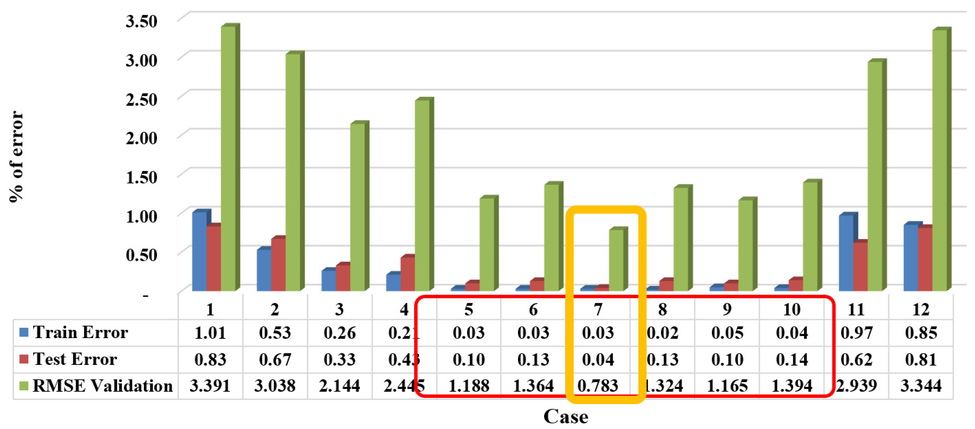
The different learning rates and split ratios are divided into 12 cases, as shown in Table 5. Figure 4 and Figure 5 show the comparison results for the different cases (LSTM model and Bi-LSTM model) in order to compare the best results.
Figure 4 and Figure 5 compare error results for our LSTM and Bi-LSTM models at different learning rates and split ratios. In cases 5 to 10 (the red box in Figure 4), the values of training error, test error, and RMSE validation error are quite low, indicating that the models perform well. When the LSTM model is compared to six cases (cases 5–10), case 5 has a lower train error, test error, and RMSE validation than the others, indicating that the LSTM model’s training performance is a 0.03% error, a 0.08% error, and a 1.057% RMSE error. A comparison of the Bi-LSTM model across six cases shows that case 7 (the yellow box in Figure 5) has a lower train error, test error, and RMSE validation than the others (cases 5 to case 10). This means that the Bi-LSTM model has a training error of 0.03%, a testing error of 0.04%, and a model validation error of 0.783%. As shown in Case 5, the appropriate learning rate and split ratio values for the LSTM model are 0.001, 70% (for training), and 30%, respectively (for testing); see the yellow box in Figure 4. The appropriate learning rate and split ratio values for the Bi-LSTM model are 0.0001 and 70% (for training) and 30% (for testing), respectively, as shown in case 7 (see the yellow box in Figure 5).
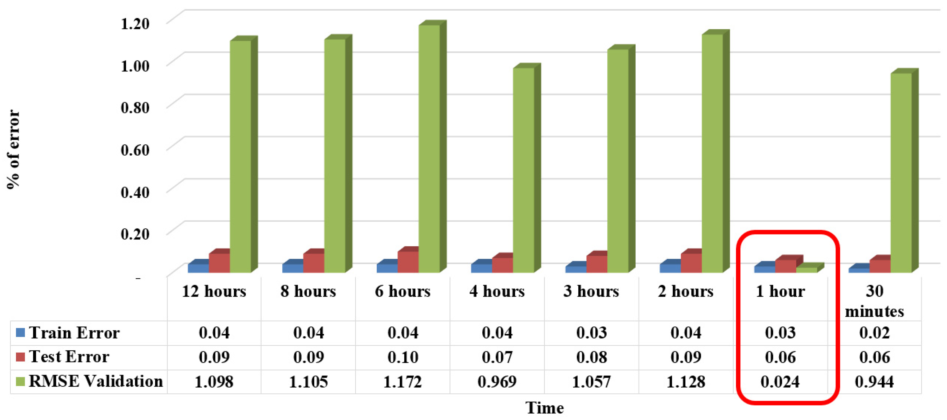
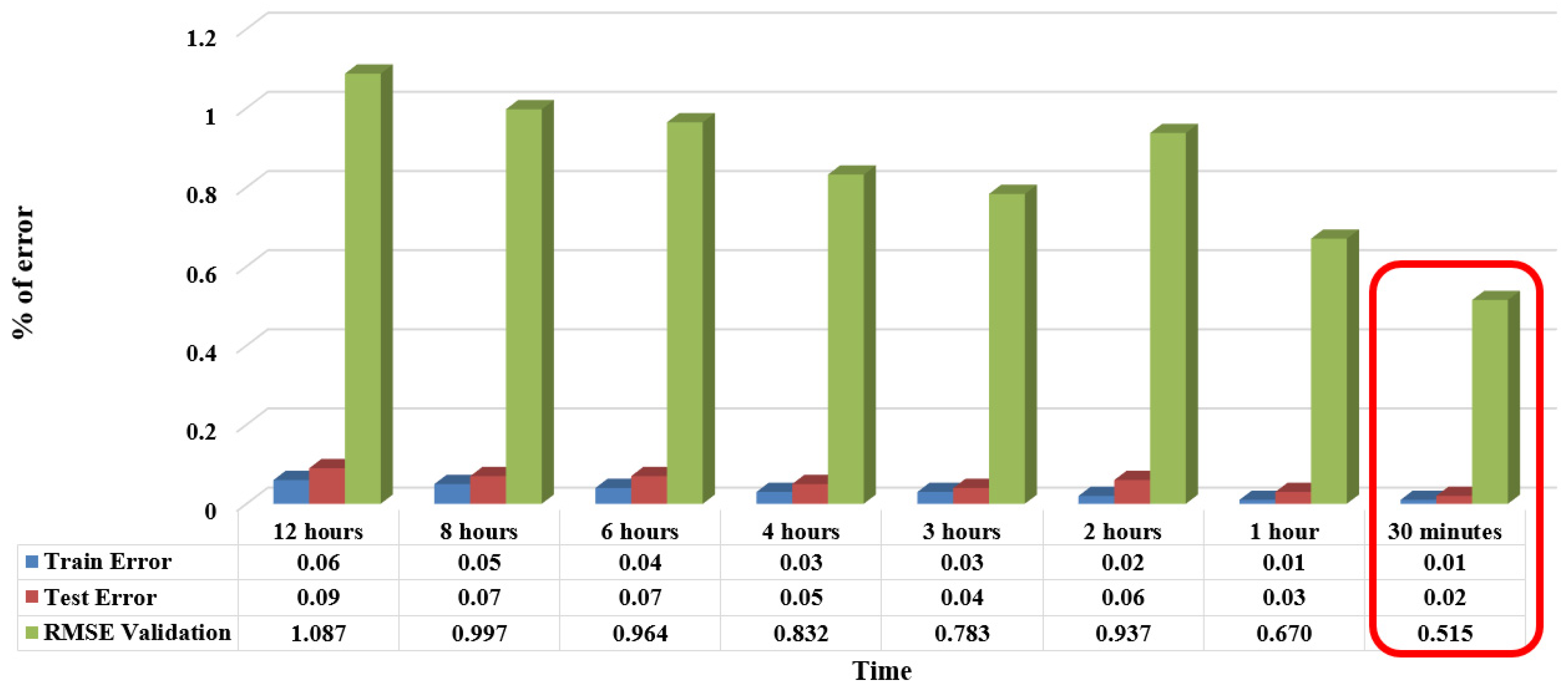
Following the selection of appropriate learning rate and split ratio values, the prediction model is tested with different time intervals that include forecasting for the next 12 h, 8 h, 6 h, 4 h, 3 h, 2 h, 1 h, and 30 min, with the error results shown in Figure 6 and Figure 7.
Figure 6 and Figure 7 show the error results of forecasting soil moisture values over different time intervals using the LSTM and Bi-LSTM models, respectively. The LSTM model is expected to perform well in the next hour, with a training error rate of 0.03%, a testing error rate of 0.06%, and a validation error rate of 0.024% (see the red box in Figure 6). In contrast, the Bi-LSTM model is expected to perform well in the next 30 min, with a training error of 0.01%, a testing error of 0.02%, and a validation error of 0.515% RMSE (see the red box in Figure 7).
As a result, the soil moisture forecasting model with LSTM and Bi-LSTM models is chosen for the next 1 h and 30 min, as shown in Figure 8 and Figure 9.
Figure 8 and Figure 9 illustrate the results of forecasting soil moisture values for the next hour (LSTM model) and 30 min (Bi-LSTM approach). When compared to measurements and soil moisture value forecasting, the results in Figure 8 and Figure 9, both models perform well in predicting soil moisture value, with approximately 0.06% and 0.15% of soil moisture value error predicted using the LSTM and Bi-LSTM models, respectively. To estimate validity of the performance of the models, K-fold cross-validation is used, and the total effectiveness of our LSTM and Bi-LSTM models is calculated by averaging the results of all five folds, as shown in Table 8.
Table 7 compares measured and predicted soil moisture values, as well as error estimation results from our LSTM and Bi-LSTM models using K-Fold cross-validation. In both the LSTM and Bi-LSTM models, the error discrepancy between measured and predicted soil moisture values is quite small, according to the results. The LSTM model, on the other hand, has a larger error between predicted and measured soil moisture values than the Bi-LSTM model. In terms of cross-validation error, the LSTM results in all five trials, as well as the averaged overall error estimation, are lower than Bi-LSTM, which is a 0.72% RMSE error and a 0.52% cross-validation error. The RMSE error for Bi-LSTM is 0.76%, and the cross-validation error is 0.57%.
The proposed soil moisture forecasting using LSTM and Bi-LSTM models accurately predicts soil moisture value, according to the results. However, while modeling the proposed model, we had to test the learning rate in each case individually using the Adam optimizer, which took some time. The Adam optimizer is, even still, working on the proposed model’s construction; however, the Adam optimizer works best on different datasets and requires drastically different learning rate schedules. Furthermore, these two models use a small dataset for training, testing, and validation, which may have an impact on model performance, and they use data from a single location.

4. Conclusions and Future Works

Water management for crop production is a difficult subject with implications for water sustainability. However, managing this resource is costly, requiring the use of numerous hardware tools, such as soil sensors, to effectively manage crop irrigation. In this paper, we proposed a novel method for estimating soil moisture in the context of crop production water management. We use machine learning to forecast soil moisture in the future using the output of low-cost IoT sensors. We propose a soil moisture forecasting model with Long-Short Term Memory based on our deep learning approach (LSTM). The data we use to train and validate our model were collected on a testbed in the Thai province of Chiang Mai. An array of IoT sensors, including a soil sensor, a water sensor, an air sensor, and a weather station, is used to collect data. An extensive data preprocessing step is performed to clean the collected data. The LSTM model we propose uses environmental indicators to predict future soil moisture based on farm environmental data. Our model was extensively tuned, and we tested various setups and architectures. In the future, more datasets will be used to estimate the performance of our models. In addition, we will put our model through its paces in various locations to see how well it performs. The data we used are available at https://github.com/SFDataset/DataSet.git (accessed on 6 December 2021) (see an Appendix A).

Author Contributions

Conceptualization, P.S. (Paweena Suebsombut); Data curation, P.S. (Pradorn Sureephong) and A.B. (Abdelhak Belhi); Funding acquisition, A.S. and A.B. (Abdelaziz Bouras); Investigation, A.S.; Methodology, P.S. (Paweena Suebsombut) and A.S.; Software, A.B. (Abdelhak Belhi); Supervision, A.S., P.S. (Pradorn Sureephong) and A.B. (Abdelaziz Bouras); Writing—original draft, P.S. (Paweena Suebsombut); Writing—review & editing, A.B. (Abdelhak Belhi) and A.B. (Abdelaziz Bouras). All authors have read and agreed to the published version of the manuscript.

Data Availability Statement

The dataset presented in this paper is available at: https://github.com/SFDataset/DataSet.git.

Acknowledgments

The authors would like to express their gratitude to DISP laboratory and SUNSpACe project 598748-EPP-1-2018-1-FR-EPPKA2-CBHE-JP (2018-3228/001-001), and acknowledge the support of Université Lumière Lyon 2 (France), Chiang Mai University—College of Arts Media and Technology (Thailand), and Qatar University. This publication was also made possible by NPRP Grant No. NPRP11S-1227-170135 from the Qatar National Research Fund (a member of Qatar Foundation), Qatar.

Conflicts of Interest

The authors declare no conflict of interest.

Appendix A. Dataset

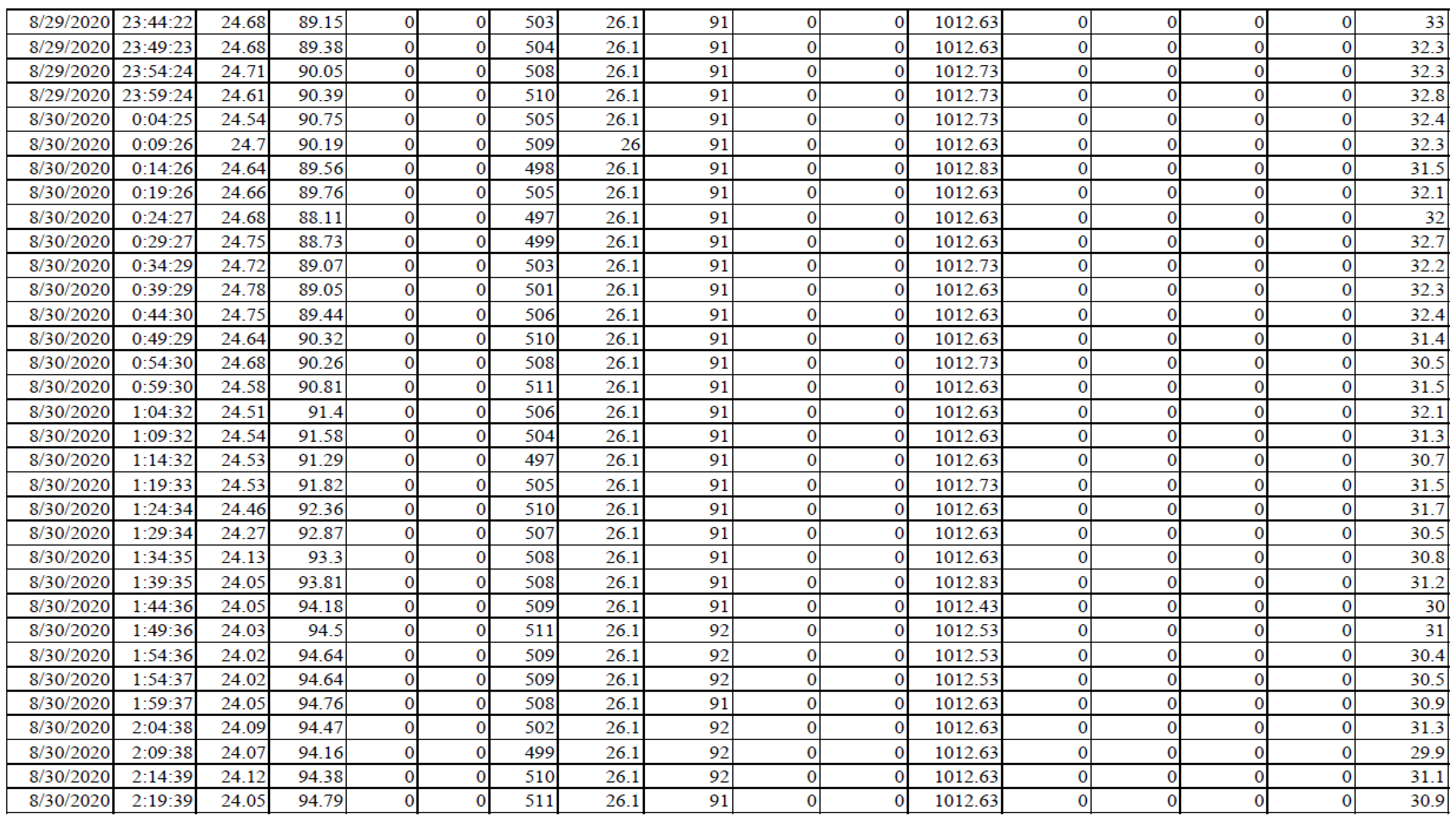
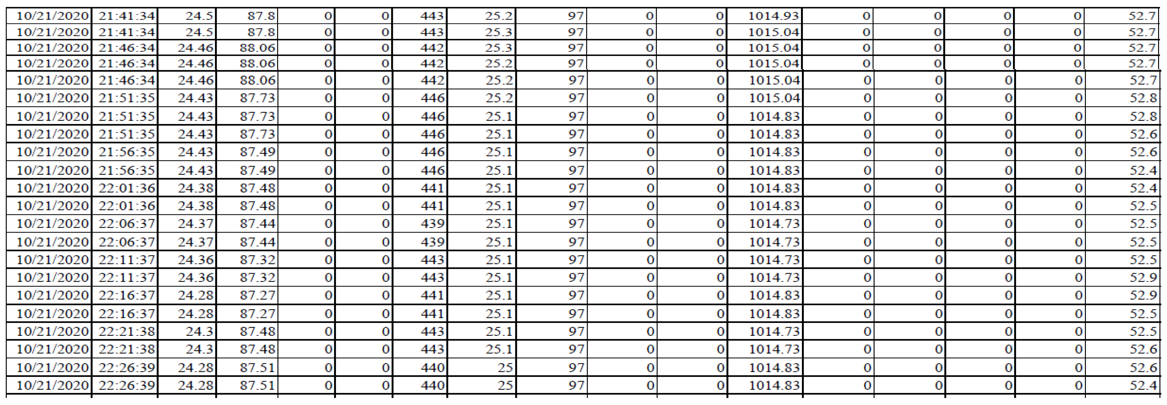
This is a sample from the used dataset (incomplete dataset) that cut the partial of the first page, middle page, and the last page of dataset. The whole dataset (3530 KB/total no. of line = 47,013 lines/1425 pages) will be available for public download on https://github.com/SFDataset/DataSet.git upon the publication of the paper.
Applsci 11 11820 i001Applsci 11 11820 i002Applsci 11 11820 i003

References

  1. IndiaAgroNet. Importance of Water Management in Crop Production. Available online: https://www.indiaagronet.com/indiaagronet/water_management/water_3.htm (accessed on 16 October 2021).
  2. Devanand Kumar, G.; Vidheya Raju, B.; Nandan, D. A Review on the Smart Irrigation System. J. Comput. Theor. Nanosci. 2020, 17, 4239–4243. [Google Scholar] [CrossRef]
  3. Khan, G.; Dhakate, K.; Kambe, S.; Meshram, S.; Lunge, A. A Review on Arduino Based Smart Irrigation System. IJSRST 2018, 4, 623–630. [Google Scholar]
  4. FAO AQUASTAT. FAO’s Global Information System on Water and Agriculture. Available online: https://www.fao.org/aquastat/en/overview/methodology/water-use (accessed on 16 October 2021).
  5. Sarah Massingham. World Water Usage Made by Sarah Massingham—Home. Available online: https://waterusagecqu.weebly.com/ (accessed on 16 October 2021).
  6. Chart: Globally, 70% of Freshwater Is Used for Agriculture. Available online: https://blogs.worldbank.org/opendata/chart-globally-70-freshwater-used-agriculture (accessed on 16 October 2021).
  7. OECD. Environmental Outlook to 2050: What Could the Environment Look Like in 2050? 2012. Available online: https://www.oecd.org/env/indicators-modelling-outlooks/49846090.pdf (accessed on 16 October 2021).
  8. Oukaira, A.; Benelhaouare, A.Z.; Kengne, E.; Lakhssassi, A. FPGA-Embedded Smart Monitoring System for Irrigation Decisions Based on Soil Moisture and Temperature Sensors. Agronomy 2021, 11, 1881. [Google Scholar] [CrossRef]
  9. Bozdemir, M.; Bayramoğlu, Z.; Ağızan, K.; Ağızan, S. Prudential Expectation Analysis in Maize Production. Turk. J. Agric.-Food Sci. Technol. 2019, 7, 390–400. [Google Scholar] [CrossRef]
  10. Lamm, F.R.; Rogers, D.H. The Importance of Irrigation Scheduling for Marginal Capacity Systems Growing Corn. Appl. Eng. Agric. 2015, 31, 261–265. [Google Scholar] [CrossRef] [Green Version]
  11. Mahlein, A.-K.; Oerke, E.-C.; Steiner, U.; Dehne, H.-W. Recent advances in sensing plant diseases for precision crop protection. Eur. J. Plant Pathol. 2012, 133, 197–209. [Google Scholar] [CrossRef]
  12. Shopping for a Smart Irrigation System? Available online: https://www.loveyourlandscape.org./expert-advice/water-smart-landscaping/smart-irrigation/shopping-for-a-smart-irrigationsyste.m/ (accessed on 16 October 2021).
  13. Adab, H.; Morbidelli, R.; Saltalippi, C.; Moradian, M.; Ghalhari, G.A.F. Machine learning to estimate surface soil moisture from remote sensing data. Water 2020, 12, 3223. [Google Scholar] [CrossRef]
  14. Cai, Y.; Zheng, W.; Zhang, X.; Zhangzhong, L.; Xue, X. Research on soil moisture prediction model based on deep learning. PLoS ONE 2019, 14, e0214508. [Google Scholar] [CrossRef] [PubMed]
  15. Hajjar, C.S.; Hajjar, C.; Esta, M.; Chamoun, Y.G. Machine learning methods for soil moisture prediction in vineyards using digital images. ICESD 2020, 167, 2004. [Google Scholar] [CrossRef]
  16. Hu, Z.; Xu, L.; Yu, B. Soil moisture retrieval using convolutional neural networks: Application to passive microwave remote sensing. Int. Arch. Photogramm. Remote Sens. Spat. Inf. Sci. 2018, 42, 583–586. [Google Scholar] [CrossRef] [Green Version]
  17. Gorthi, S.; Dou, H. Prediction models for the estimation of soil moisture content. DETC 2011, 54808, 945–953. [Google Scholar] [CrossRef] [Green Version]
  18. Karandish, F.; Šimůnek, J. A comparison of numerical and machine-learning modeling of soil water content with limited input data. J. Hydrol. 2016, 543, 892–909. [Google Scholar] [CrossRef] [Green Version]
  19. Yu, J.; Tang, S.; Zhangzhong, L.; Zheng, W.; Wang, L.; Wong, A.; Xu, L. A Deep Learning Approach for Multi-Depth Soil Water Content Prediction in Summer Maize Growth Period. IEEE Access. 2020, 8, 199097–199110. [Google Scholar] [CrossRef]
  20. Fang, K.; Kifer, D.; Lawson, K.; Shen, C. Evaluating the potential and challenges of an uncertainty quantification method for long short-term memory models for soil moisture predictions. Water Resour. Res. 2020, 56, e2020WR028095. [Google Scholar] [CrossRef]
  21. Zhang, D.; Zhang, W.; Huang, W.; Hong, Z.; Meng, L. Upscaling of surface soil moisture using a deep learning model with VIIRS RDR. ISPRS Int. J. Geo-Inf. 2017, 6, 130. [Google Scholar] [CrossRef]
  22. Ge, L.; Hang, R.; Liu, Y.; Liu, Q. Comparing the performance of neural network and deep convolutional neural network in estimating soil moisture from satellite observations. Remote Sens. 2018, 10, 1327. [Google Scholar] [CrossRef] [Green Version]
  23. Song, X.; Zhang, G.; Liu, F.; Li, D.; Zhao, Y.; Yang, J. Modeling spatio-temporal distribution of soil moisture by deep learning-based cellular automata model. J. Arid Land. 2016, 8, 734–748. [Google Scholar] [CrossRef] [Green Version]
  24. Samaya Madhavan, M. Tim Jones, Deep Learning Architectures, The Rise of Artificial Intelligence. 2021. Available online: https://developer.ibm.com/articles/cc-machine-learning-deep-learning-architectures/ (accessed on 15 October 2021).
  25. Mohammad-Parsa, H.; Lu, S.; Kamaraj, K.; Slowikowski, A.; Haygreev, C.V. Deep learning architectures. In Deep learning: Concepts and Architectures; Springer: Berlin/Heidelberg, Germany, 2019; pp. 1–24. [Google Scholar]
  26. Yu, Y.; Si, X.; Hu, C.; Zhang, J. A review of recurrent neural networks: LSTM cells and network architectures. Neural Comput. 2019, 31, 1235–1270. [Google Scholar] [CrossRef] [PubMed]
  27. Pedregosa, F.; Varoquaux, G.; Gramfort, A.; Michel, V.; Thirion, B.; Grisel, O.; Blondel, M.; Prettenhofer, P.; Weiss, R.; Dubourg, V. Scikit-learn: Machine learning in Python. J. Mach. Learn. Res. 2011, 12, 2825–2830. [Google Scholar]
  28. Chollet, F. Keras: Deep Learning Library for Theano and Tensorflow. Available online: https//keras.io (accessed on 16 October 2021).
Figure 1. Methodology of the proposed soil moisture forecasting model.
Applsci 11 11820 g001
Figure 2. Multiple sensors installed for data collection (1 set of soil moisture sensors, 1 set of air indoor sensors, 1 weather station, and 1 set of water sensors).
Applsci 11 11820 g002
Figure 3. Proposed model architecture.
Applsci 11 11820 g003
Figure 4. Error results comparison of the Soil Moisture value forecasting in different cases of learning rate (LR) and split ratio (SR)—LSTM model.
Applsci 11 11820 g004
Figure 5. Error results comparison of the Soil Moisture value forecasting in different cases of learning rate (LR) and split ratio (SR)—Bi-LSTM model.
Applsci 11 11820 g005
Figure 6. Comparison error results of the Soil Moisture value forecasting in different time intervals (LSTM model).
Applsci 11 11820 g006
Figure 7. Comparison error results of the Soil Moisture value forecasting in different time intervals (Bi-LSTM model).
Applsci 11 11820 g007
Figure 8. Result of soil moisture value forecasting for (a) the next 1 h and (b) the next 30 min.
Applsci 11 11820 g008
Figure 9. Zoom in of the red box in Figure 8 (a) and Figure 8 (b).
Applsci 11 11820 g009
Table 1. Collected data and their purpose.
No.Data FieldPurpose
1Soil MoistureThe historical collected soil moisture value will be used for retraining the proposed forecasting model.
2Soil TemperatureThe historical collected soil temperature value will be used to train/retrain the proposed model. And the real-time soil temperature value will be used to predict the future value of soil moisture.
3Indoor: Air TemperatureThe air indoor temperature indicates the air temperature inside the greenhouse.
4Indoor: Relative HumidityThe indoor relative humidity indicates the air moisture inside the greenhouse that helps in making a decision for irrigation.
5Indoor: Light IntensityThe indoor light intensity indicates the temperature and relative humidity inside the greenhouse.
6Indoor: UV indexThe UV index value impacts the temperature and relative humidity inside the greenhouse.
7Outdoor: Air TemperatureThe air outdoor temperature indicates the air temperature outside the greenhouse.
8Outdoor: Relative HumidityThe outdoor relative humidity indicates the air moisture outside the greenhouse.
9Outdoor: Light IntensityThe outdoor light intensity impacts the temperature and relative humidity outside the greenhouse.
10Outdoor: UV indexThe UV index value also impacts the temperature and relative humidity outside the greenhouse.
11Outdoor: Wind SpeedThe wind speed value indicates the speed of wind outside the greenhouse that may impact the wind flow inside the greenhouse.
12Outdoor: Wind DirectionThe wind direction indicates the direction of wind outside the greenhouse.
13Outdoor: Precipitation RateThe precipitation rate indicates the rate of rainfall at that time.
14Outdoor: Precipitation TotalThe precipitation total indicates the total amount of rainfall in one day.
Table 2. Sample of the collected raw data.
DateTimeIndoor DataOutdoor DataOutput
Temp
(°C)
Humid
(%)
UVluxCO2Temp
(°C)
Humid
(%)
Wind Speed
(mph)
Wind Gust
(mph)
Air Pressure
(in)
Precop. Rate
(in)
Precip. Accum.
(in)
UVSolar
(w/m2)
Soil Moisture
(%)
6/3/20209:05:3028.1137.810.366359931.39360029.88000063.1
6/3/20209:06:4427.9237.560.367059931.39360029.89000062.2
6/3/20209:11:4527.335.380.361023059931.28360029.89000062.7
6/3/20209:19:1628.3870.190.07100047531.28360029.89000062.6
6/3/20209:24:1632.8155.131.873514047531.22360029.89000062.2
6/3/20209:29:1734.4152.343.785461246331.22360029.89000062.2
6/3/20209:34:1734.6548.954.145461243531.11370029.89000062.3
6/3/20209:44:1935.6445.964.465461241431.06370029.89000062
6/3/20209:49:2034.7950.781.31780040431370029.9000061.5
6/3/20209:54:2035.5446.951.913044341430.94370029.9000061.5
6/3/20209:59:2135.1648.931.312348346030.89370029.9000062.5
6/3/202010:04:2135.5247.371.191457647030.78370029.9000062.5
6/3/202010:09:2235.9346.121.331722647530.78370029.89000062.9
6/3/202010:14:2236.1346.721.673200046130.72370029.89000062.6
6/3/202010:19:2336.3845.482.533136045730.67370029.89000063
6/3/202010:24:2336.6745.0822400044430.61370029.89000062.7
6/3/202010:29:2436.4546.151.431688346530.56370029.89000062.7
6/3/202010:34:2436.5447.521.612167344730.5370029.89000062.6
6/3/202010:39:2536.2845.842.412950045530.39370029.89000062.4
6/3/202010:44:2536.3646.362.43727047430.39370029.89000062.8
6/3/202010:49:2636.5146.172.872949344730.28380029.88000062.3
6/3/202010:54:263746.313.834813345830.22380029.88000063.4
6/3/202010:59:2737.0545.832.073020645230.22380029.88000062.9
6/3/202011:04:2836.7346.133.594335341330.11380029.88000062.3
Table 3. Descriptive statistics for the dataset.
VariableMeanStandard ErrorMedianStandard DeviationVarianceMinimumMaximumValidMissing
Date44017.053130.1406556744401718.73890461351.1465464398544049177490
Time0.4956319040.0021847240.4940509260.2910606210.0847162854.63E-050.999930556177490
Indoor temp29.833095390.03779975327.935.03588618125.3601496223.2747.41177490
Indoor humid75.647511970.14484982379.9619.29767169372.400132725.64100177490
Indoor UV0.9058358220.0109871660.081.4637692922.14262053907.72177490
Indoor lux11568.96558130.404669193317373.21068301828449.3054612177490
CO2 indoor533.26254090.38400260353651.148800812616.199824309715177490
Outdoor temp27.800673840.01636145127.392.1797603734.75135528223.8939.22177427
Outdoor humid50.682235620.1141578584715.20872326231.30526313399177490
Outdoor wind speed0.0113471180.00057897400.0771340850.00594966701.4177490
Outdoor wind gust0.0227224070.00103152900.1374257960.01888584902.4177490
Outdoor Pressure29.85817680.00052475429.870.0699105970.00488749229.630.01177490
Outdoor Precip. Rate0.00570680.00066513400.0886127710.00785222303.78177490
Outdoor Precip. Accum0.0441422050.00220221200.2933904790.08607797302.7177490
Outdoor UV0.0853569220.00464467100.6187880050.382898595010177490
Outdoor Solar11.270865960.527558327070.284154914939.86243101102.3177490
Soil moisture56.211009070.02018138556.12.6886726067.2289603850.787.9177490
Table 4. Sample of the processed data.
Indoor TempIndoor HumidIndoor UVIndoor luxIndoor CO2Outdoor TempOutdoor HumidOutdoor UVOutdoor SolarSoil Moisturecos_Timessin_Times
028.1137.810.3663599.031.393600.063.1−0.7238710.689935
127.9237.560.3670599.031.393600.062.2−0.7275730.686030
227.3035.380.3610230599.031.283600.062.7−0.7424140.669941
328.3870.190.071000475.031.283600.062.6−0.7639840.645235
432.8155.131.8735140475.031.223600.062.2−0.7778780.628416
Table 5. The best hyperparameters based on our empirical study.
HyperparametersLRSREpochInput Time StepsFuture StepsBatch Size
Value0.0180% Train
20% Test
1003001272
Value0.00170% Train
30% Test
1003001272
Value0.000180% Train
20% Test
1003001272
Table 6. List of 12 different cases of learning rates and split ratios to define the suitable values of the proposed model.
CaseLearning Rate (LR)Split Ratio (SR)CaseLearning Rate (LR)Split Ratio (SR)
10.170% (train), 30% (test)70.000170% (train), 30% (test)
20.180% (train), 20% (test)80.000180% (train), 20% (test)
30.0170% (train), 30% (test)90.0000170% (train), 30% (test)
40.0180% (train), 20% (test)100.0000180% (train), 20% (test)
50.00170% (train), 30% (test)110.00000170% (train), 30% (test)
60.00180% (train), 20% (test)120.00000180% (train), 20% (test)
Table 7. Prediction in different time steps and time intervals.
Time Interval Time StepsSoil Moisture Value (%)RSME Validation (%)
MeasureForecastStatic Error
12 h14457.8055.702.102.595
8 h9657.0054.902.102.466
6 h7256.2054.501.702.380
4 h4855.9054.701.202.216
3 h3654.9054.700.202.096
2 h2455.7055.850.152.009
1 h1255.4054.530.131.779
30 min655.7055.650.051.637
Table 8. Comparison of cross-validation result of soil moisture forecasting model (LSTM and Bi-LSTM).
Next 1 h
(LSTM)
Next 30 min
(Bidirectional LSTM)
1. Soil moisture value: Measure55.64%55.70%
2. Soil moisture value: Forecast55.70%55.55%
3. Cross Validation (CV) results
   3.1. Round 1
    -RSME loss0.62%0.66%
    -CV loss0.38%0.42%
   3.2. Round 2
    -RSME loss0.75%0.79%
    -CV loss0.56%0.60%
   3.3. Round 3
    -RSME loss0.78%0.82%
    -CV loss0.61%0.65%
   3.4. Round 4
    -RSME loss0.77%0.81%
    -CV loss0.60%0.66%
   3.5. Round 5
    -RSME loss0.69%0.73%
    -CV loss0.48%0.54%
   3.6. Averaged overall error estimation
    -RSME loss0.72% (+/−0,06%)0.76% (+/−0,06%)
    -CV loss0.52% (+/−0,08%)0.57% (+/−0,08%)
Publisher’s Note: MDPI stays neutral with regard to jurisdictional claims in published maps and institutional affiliations.