Computational Modeling of the Thermal Behavior of a Greenhouse

Abstract

The need for production of all kinds of crops in high quantities and over the entire year makes the agricultural sector one of the major energy consumers. The optimization of this consumption is essential to guarantee its sustainability. The implementation of greenhouses is a strategy that allows assurance of production needs and possesses large optimization potential for the process. This article studies different greenhouse structures by computational simulation using EnergyPlus and DesignBuilder. First, a comparison was performed between the computational results and the measured values from a greenhouse prototype at different operating conditions. Overall, the comparison shows that the computational tool can provide a reasonable prediction of the greenhouse thermal behavior, depending on the differences between the weather data modeled and observed. An outdoor air temperature difference of 16 °C can cause a difference of about 10 °C between the air temperature predicted and measured inside the greenhouse. Subsequently, a selected set of case studies was developed in order to quantify their influence on the thermal performance of the greenhouse, namely: the greenhouse configuration and orientation; the variation of indoor air renewal; changes to the characteristics of the roof; the effect of the thermal mass of the walls; and location of the greenhouse. The results show that a correct greenhouse orientation, together with a polyethylene double cover with a 13 mm air layer, a granite wall of 40 cm thickness on the north wall, and variable airflow rate, may lead to a reduction of the greenhouse energy consumption by 57%, if the greenhouse is located in Lisbon, or by 43%, if it is located in Ostersund, during the harshest months of the heating season.

1. Introduction

A greenhouse allows the creation of a controlled environment with proper microclimate conditions required for crop growth, increasing crop production rates and quality [1]. Parameters such as indoor air temperature, soil temperature, relative humidity, light intensity, and carbon dioxide concentration can be controlled using a greenhouse. As greenhouses allow cultivation in areas where the natural conditions are unfavorable for plant growth, they may avoid the need to transport vegetables and horticultural crops from distant places [2]. Greenhouses are also being used worldwide for drying, with many advantages concerning the quality of the dry products when compared to traditional drying methods. In this specific case, products are spread on the ground, exposing them directly to solar radiation, with considerable losses due to dirt, dust, insects, microorganisms, animals, and birds [3].

Parameters such as greenhouse shape, the materials used in its construction, orientation, and management systems can have a large impact on the greenhouse’s performance. Therefore, optimizing greenhouses is truly important to ensure their contribution to the sustainability of food production.

The evolution of computational power allows numerical modeling to be used to study these structures while also keeping cost and resource requirements low, when compared with developing physical prototypes. Empirical evidence is, nevertheless, a requirement in numerical modeling as a means to assess the reliability of the simulation results. Recent studies show that various building characteristics can have a significant impact on the energy required to keep the conditions inside a greenhouse suitable for crop growth. An optimization procedure integrating a dynamic thermal model that was developed for optimal design of solar greenhouses in different climate conditions revealed that an optimal solar greenhouse can work passively 85% of the time over a year without additional energy sources [4].

The shape of the roof of the greenhouse can reduce the heating demand by up to 4.2% [5]. East–west orientation can lower energy requirements of a greenhouse operating year-round [6]. The usage of a greenhouse cover with higher insulating properties was able, through computer simulations in EnergyPlus, to decrease energy consumption by more than 30% [7]. Ansys Fluent simulations also demonstrated the benefits of carefully selecting the greenhouse cover [8]. The various design characteristics of a greenhouse that result in higher efficiency in the situation under study are not always applicable to every other greenhouse that is being optimized, such as the orientation of the structure, the optimal value of which varies with the latitude of the site where the greenhouse will be implemented [9,10]

The microclimates that develop around and between the crop canopies require very detailed modeling and, consequently, high computational power. However, there has been success in replicating these thermal interactions in numerical models [11], with simulations of microclimates being useful to optimize plant pot position and frequency of movement, resulting in a reduction by 90% in microclimate formation and a 95% reduction in frequency of pot movement [12]. To obtain numerical model results that better match the real-world conditions experienced inside a greenhouse during crop development, it has been shown that modeling not only the structural components of the greenhouse but also the crops themselves is a valuable aspect of the simulation process [13,14].

While existing computer software has shown to be capable of assessing the thermal behavior of a greenhouse, research has been done to develop tools that are capable of outputting better results, with an application based on TRNSYS showing discrepancies of 50 kWh/m³ comparatively with traditional EnergyPlus simulations [15]. Mathematical models that were developed for specific greenhouse assessment and subsequently solved with the computer application MATLAB/Simulink have also demonstrated ability to correctly estimate the thermal performance of a greenhouse [16].

In this paper, a computational model of an existing small-scale greenhouse was built using the computer software EnergyPlus and DesignBuilder. The model was then simulated under the same conditions that were applied to the physical greenhouse to evaluate the reliability of the simulation results. Subsequently, a group of case studies was defined to evaluate the impact of different design choices in the thermal behavior of the greenhouse.

2. Materials and Methods

2.1. Experimental Setup

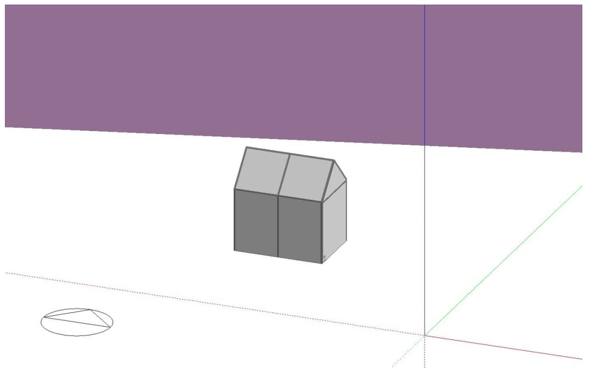
The greenhouse under study is located in the city of Covilhã at the University of Beira Interior Engineering Faculty campus in the center-east region of Portugal, having the following GPS coordinates: 40°16′43″ N 7°30′48″ W.

The greenhouse has a rectangular base with a traditional gable roof, with exterior dimensions of 2.0 m × 1.4 m × 2.1 m (length × width × height). Figure 1 shows in more detail the supporting structure of the greenhouse and its dimensions.

The supporting structure is made from fir wood, with cross-sectional dimensions of 30 mm × 30 mm. The cover, which involves all sides of the greenhouse, is made of a commercial polyethylene 215 μm in thickness commonly used for this kind of greenhouse. Figure 2 shows the greenhouse with the covering material assembled.

The greenhouse has two circular openings of 127 mm in diameter located in the bottom-left corner of the south-facing wall and the top-right corner of the north-facing wall to allow natural or forced ventilation of the interior of the greenhouse. Figure 3 shows one of these openings with a mechanical ventilator duct attached.

The greenhouse location is surrounded by various buildings and a retaining wall that are tall enough to influence its thermal performance by blocking sunlight during certain periods of the day.

Temperature and relative humidity data acquisitions were performed by means of two devices, the PCE-T 1200 temperature data logger, using T-type thermocouples (Omega Engineering Inc., Norwalk, CT, USA) and the Lascar Electronics EL-USB-1-LCD portable data logger. The accuracies of the temperature and relative humidity measurements were ±0.55 °C and 2.25%, respectively. In order to ensure stable thermal conditions inside the greenhouse, it was necessary for some tests to use a heating device. The equipment used was a ceramic fan heater with a digital thermostat and maximum power of 1800 W.

The experimental type A tests included natural and forced ventilation inside the greenhouse. Some tests (type B) included a heating set-point temperature to ensure a minimum value of the internal air temperature by using an auxiliary heater located in the greenhouse. Type C tests included a low airflow rate inside the greenhouse with outside fresh air but keeping the auxiliary air heater turned off.

Table 1. Experimental test parameters necessary for model validation [17,18].

Tests	Ventilation Type	Airflow Rate (ac/h)	Auxiliary Heating	Heating Set-Point (°C)
A1	Natural	-	OFF	-
A2	Forced	12.9	OFF	-
A3	Forced	14.7	OFF	-
A4	Natural	-	OFF	-
B5	Natural	-	ON	12
B6	Natural	-	ON	20
B7	Forced	12.9	ON	18
C1	Forced	1.0	OFF	-
C2	Forced	3.0	OFF	-
C3	Forced	3.0	OFF	-

lists the parameters of each of the experimental tests. The experimental tests were each conducted over 24 h, and the air temperature and relative humidity were recorded every 10 min. Additional details of the experimental apparatus and experimental tests can be found in [17,18].

2.2. Computational Model

The computer application EnergyPlus version 8.1 with graphical user interface DesignBuilder version 3.4.041 was used to simulate the dynamic thermal behavior of the greenhouse model. This well-known computational tool was developed and applied mostly for more traditional structures, such as residential, office, and commercial buildings [19,20,21,22,23]. However, it has been used successfully in simulating considerably different structures from the aforementioned ones, such as data centers, outdoor telecommunications cabinets, or greenhouses [19,24,25].

Figure 4 and Figure 5 show the model of the greenhouse under study and its surrounding structures in order to include the shadow effects on the greenhouse during certain periods of the day.

With the model’s geometry defined, the following step was to set the building material’s characteristics in the model. As such, the extensive library of material templates included with DesignBuilder was used for most of the greenhouse’s materials. For the supporting wood structure, the template “Woods-fir, pine” was selected and modified to have a thickness of 0.03 m. This template was applied to the “External walls”, “Pitched roof (occupied)”, and “Internal partitions” sections of the model.

The floor of the greenhouse is made from the natural terrain found in the greenhouse’s location, and so the template “Earth, common (0.5 m)” was chosen. Air infiltration was considered in this model. Although no experimental data were available—as it is a small greenhouse built with special care for research purposes and located in a place relatively sheltered from the wind—an infiltration value of 0.2 ac/h (air chamber volume changes per hour) was considered. The properties of the surrounding buildings are also relevant, and so the “Project component block material” template was set for these structures.

Table 2. Polyethylene cover properties used for the model.

Property	Value
Thickness (mm)	0.215
Thermal conductivity (W/m·K)	0.330
Solar transmittance	0.800
Outdoor solar reflectance	0.170
Inside solar reflectance	0.170
Visible transmittance	0.850
Outdoor visible reflectance	0.120
Inside visible reflectance	0.120
Infra-red transmittance	0.000
Outdoor emissivity	0.700
Inside emissivity	0.700

summarizes the characteristics of the polyethylene cover, which were inputted manually, with the thermal conductivity being sourced from the ISO 10456 standard and the other necessary properties from Kempkes et al. [18].

A climatic data file containing the weather data of Covilhã was used [26] for simulation purposes. This data file includes 2002 as the reference year. Furthermore, a “10 time steps per hour” setting was adopted, and the outdoor ambient air temperature was used as the criterion to determine which simulation day more closely matched the day of each experimental test. Additional details of the greenhouse modeling can be found in [27].

3. Results

This section includes the comparison of the results of the computational tool with the results obtained from a real greenhouse, followed by a detailed set of case studies.

3.1. Comparison with Experimental Data

Figure 6 shows the results of the simulation interval of 28 May at 17:00 to 29 May at 16:00 for the test A1, specifically the outdoor and indoor air temperatures of the greenhouse for both the experimental and the simulated results.

There was considered to be natural ventilation with an airflow of 0.2 ac/h without auxiliary heating for the dynamic simulation of the greenhouse in test A1. The trend of the indoor air temperature is similar in both numerical and experimental tests. However, the numerical predictions are above the experimental values during the night period, showing an air temperature difference between 7 °C and 10 °C. On the other hand, during the day the temperature predicted for the indoor air of the greenhouse is almost always above the value measured experimentally, although the temperature of the outdoor air measured at the site is higher than that considered for modeling purposes. It reached a maximum difference of 6.5 °C early in the day.

The comparison results for the period between 29 May at 17:00 and 30 May at 16:00, test B7, are given in Figure 7. This test includes an airflow rate of 12.9 ac/h and an auxiliary air heater with a set-point of 18 °C. The comparison shows a similar trend of the numerical and experimental indoor air temperature values. During the day, when the numerical values of the outdoor air temperature are lower than the experimental ones, a similar behavior is observed, but a temperature difference of about 10 °C is reached between numerical and experimental results of the indoor air temperature. This trend arises from the role of the airflow rate, which affects the indoor air temperature in both situations.

Figure 8 shows comparison results for the period between 25 February at 17:00 and 26 February at 16:00, test C3. In this test, there was considered to be an airflow rate of 3 ac/h without auxiliary air heater. Again, a similar trend was found. The lower value of the indoor air temperature is reached at about the same time, around 06:00. During the day, the outdoor air temperature difference between the experimental and numerical models reaches a maximum value of about 16 °C, resulting in lower values for the predictions of the indoor air temperature by about 10 °C.

Overall, the comparison results show that the computational tool can provide a reasonable prediction of the indoor air temperature of the greenhouse. However, it must pointed out that the climatic data files used in this simulation software could significantly influence the quality of the results, as observed by other authors [28,29,30].

3.2. Case Studies

Taking advantage of the potential of the computational tool employed, a selection of case studies was defined in order to understand and quantify the consequences for the greenhouse thermal behavior resulting from the change of some individual characteristics of its envelope. In all cases studies, the model equivalent to the experimental greenhouse is always taken as the reference case.

3.2.1. Geometry and Orientation

The first group of case studies analyzes the thermal behavior of a greenhouse with different overall dimensions while maintaining the same floor area and total height, when applicable, as well as the impact of the greenhouse orientation.

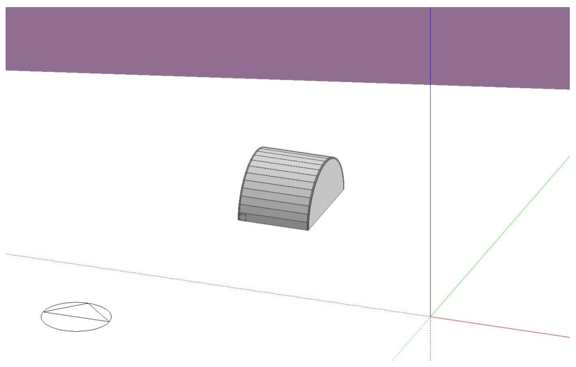
Figure 9 shows the first case study, in which a greenhouse with a cross-sectional profile of a quarter circle was adopted.

Case study 2 implemented a cross-sectional profile of a semicircle, resulting in a greenhouse with a considerably smaller internal volume, which can be seen in Figure 10.

The third case study used a similar geometry to case study 2, where the geometry of case study 2 was raised so that it had the same height at the highest point as the reference greenhouse. Figure 11 shows the third case study configuration.

In order to assess the effect of greenhouse orientation, in the last case study of this group the reference greenhouse, keeping the same dimensions, is simply rotated 90° counterclockwise, so that the initially south-facing wall is now oriented to the east, as shown in Figure 12.

The annual results of this group of case studies can be found in Figure 13 and Figure 14, which show, respectively, the indoor air temperature and relative humidity for the reference greenhouse as well as for the four case studies. The outdoor air temperature is also shown in both figures.

The results show that the different configurations tested have a worse thermal performance than the reference case. In the worst case, case study 3, the reduction in indoor air temperature goes from around 5 °C in January to 8 °C in July. Changing the orientation of the greenhouse—case study 4—makes it possible to slightly increase the indoor air temperature by around 0.8 °C in January and reduce it in July by around 1 °C.

The annual air relative humidity results show a similar but symmetrical behavior to that of the annual air temperature. The highest indoor air relative humidity of 64% is obtained in case study 3, which is 11% above the reference case, in January. The minimum air humidity value is obtained in August in the reference case with a value of 31%, which is 8% below case study 3. It can be concluded that the reference case with the orientation provided by case study 4 is the better choice in terms of greenhouse indoor air temperature behavior.

3.2.2. Airflow Rate

The second group of case studies evaluates the effect of increasing the rate of the renovation of the air inside the greenhouse by means of mechanical ventilation. The airflow rate values simulated were 1 ac/h, 2 ac/h, 3 ac/h, 4 ac/h, and 5 ac/h for case studies 5 through 9, respectively. Figure 15 and Figure 16 show the air temperature values and relative humidity values, respectively, for the second group of case studies for the simulation day of 15 January. The choice of this day is related to the fact that it is the most demanding in terms of energy consumption to provide the interior heating of the greenhouse.

As shown in Figure 16, the relative humidity values show that the increase in airflow rate resulted in a steady increase in relative humidity during the day as well as the night, with an exception in the later hours of the night when the reference greenhouse’s relative humidity was about 10% higher than any of the case studies as a result of a much lower airflow rate. It should be mentioned that in a real greenhouse, the relative humidity of the indoor air during the day would never be so low, due to the products breathing. The results show that the variation of the airflow rate allows adjustment of the temperature of the indoor air in the greenhouse, which, even on a winter day, can reach temperatures close to 30 °C at certain times of the day. A more stable relative humidity is also achievable by increasing the airflow rate.

As expected, the results show that increasing the outdoor air input results in lower temperatures during the day, reaching an air temperature difference of 6.5 °C between the 0.2 ac/h case (reference case) and the 5 ac/h case (see Figure 15). The minimum air temperature is obtained at 08:00 and varies between 2.2 °C and 2.9 °C, for the highest and lowest airflow rate, respectively. During the night, there is a reduced impact of the airflow rate on the variation of the temperature inside the greenhouse, due to the proximity between the indoor and outdoor temperatures.

3.2.3. Greenhouse Cover

Two case studies were carried out to study the effect of the characteristics of the greenhouse cover on its thermal performance. In case study 10, the greenhouse envelope is made up of two polyethylene film separated by a 13 mm layer of air. In case study 11, three polyethylene films are used instead of two but with the same thickness of air separation between them.

The air temperatures inside the greenhouse for the different types of cover over the year are given in Figure 17. The three-layer cover solution allows obtention of the highest temperature of the greenhouse’s indoor air throughout the year, surpassing the reference case, which has a simple cover, by 3.5 °C in January and 7.3 °C in July. However, the two-layer setup appears to be more cost-effective and does not excessively penalize the air temperature reached, with a temperature reduction of just 1 °C in January.

The relative air humidity results of case studies 10 and 11 are shown in Figure 18. The two- and three-layer configurations are capable of significantly reducing the relative humidity inside the greenhouse throughout the year, due to the higher air temperature reached. These two case studies allow us to conclude that the quality of the greenhouse cover also plays a relevant role in the thermal conditions reached inside the greenhouse.

3.2.4. Outer-Facing Side Cover Emissivity

The fourth group of case studies focuses on the emissivity value of the outer-facing side of the greenhouse cover. Case studies 12 through 15 change this parameter to 0.1, 0.3, 0.5, and 0.9, respectively. Figure 19 and Figure 20 contain the temperature and relative humidity results for these case studies.

As expected, the difference of relative humidity inside the greenhouse between the reference case and the lowest emissivity case decreased is 7.4% in January and 5.0% in July, due to the correlation between air temperature and relative air humidity. See Figure 20 for the variation of relative humidity during the year.

This group of case studies shows that by decreasing the emissivity value on the outside of the polyethylene cover, there is an increase in the indoor air temperature of the greenhouse, reaching 2.9 °C in January and 5 °C in July for an emissivity value of 0.1 in relation to the reference case. This indoor air temperature increase is due to the reduction in infrared radiation escaping from the interior through the cover.

3.2.5. North-Facing Wall Material and Thickness

In order to evaluate the role of the thermal mass in the thermal performance of the greenhouse, solid granite rock walls with 40 cm, 60 cm, and 100 cm thicknesses were considered for the north-facing wall. The “grounded” boundary condition was also applied, meaning the outer edge of the granite is in contact with ground terrain/soil instead of outdoor ambient air.

The results of indoor air temperatures of the greenhouse for these case studies are shown in Figure 21 and Figure 22, respectively, for the middle days of January and July.

The July values show that the wall thickness affects the obtained air temperatures, with the minimum value, at 05:00, increasing from 21.4 °C to 23.7 °C when the wall thickness increases from 40 to 100 cm. At 14:00, the maximum indoor air temperature of the greenhouse shows a difference of 2 °C between the maximum and minimum wall thicknesses but, in any case, below the temperature of 56.7 °C of the reference case at the same time. In January, the thermal mass of the granite wall allows the minimum indoor air temperature of the greenhouse, reached at 08:00, to be 3.6 °C above the reference greenhouse and 6.3 °C above the outdoor temperature regardless of the thickness considered for the wall. The maximum indoor air temperature reached at 15:00 is similar to the reference greenhouse’s value and is also unaffected by the thickness of the granite wall, remaining at 23.7 °C above the outdoor ambient temperature at that time.

Overall, the air temperature values show the ability of the high thermal inertia of the large granite wall to act as a heat reservoir that releases heat during the colder periods and absorbs heating during the hotter ones. However, it also shows that the wall thickness should be balanced with a careful airflow rate to limit the maximum air temperatures reached.

3.2.6. Geographical Location

The final group of case studies consists in simulating the reference greenhouse in various locations of the globe so as to assess its performance and limitations in different climates. Case studies 19 to 21 have the reference greenhouse set in Lisbon, Moscow, Ostersund, and Riyadh, respectively. Figure 23 and Figure 24 show the results of these case studies for the day of 15 January, and Figure 25 and Figure 26 contain the results for the day of 15 July.

As shown in Figure 24, the relative humidity values for 15 January demonstrate that Moscow and Riyadh have a more constant relative humidity throughout the day, although reaching relatively high and low values, respectively. Ostersund and Lisbon have a wider range of values, with Lisbon having bigger oscillations but not surpassing the highest and lowest values of all case studies.

The temperature results in January show that the greenhouse mostly requires heat extraction during the day when located in Lisbon and Riyadh in order to achieve an adequate temperature for operation. When located in Moscow and Ostersund, constant auxiliary heating is necessary to achieve an appropriate temperature in the greenhouse. Thus, this greenhouse is better suited for warmer climates if winter operation is required.

The air temperature results for 15 July shown in Figure 25 allow us to conclude that the greenhouse reaches very high temperatures in Lisbon and, especially, Riyadh, meaning that constant heat extraction will be necessary to achieve adequate temperature levels for any kind of crop development. Moscow’s and Ostersund’s temperature values show that the greenhouse is very suitable for these locations, as it able to maintain a much more constant and adequate temperature throughout the day.

As shown in Figure 26, the relative humidity values for case studies 19 to 21 show the greenhouse, when located in Riyadh, having a very constant and low relative humidity level, followed by Ostersund, where a larger range but average relative humidity values are observed, and, lastly, with Lisbon and Moscow showing the largest oscillation as the day progresses. This set of case studies shows that the reference greenhouse’s capabilities depend not only on the location but also on the season. The reference greenhouse’s low insulation mean that additional energy sources will be necessary to provide more adequate ambient conditions, particularly if the greenhouse is to be operated during the entire year.

3.2.7. Greenhouse Energy Consumption

In this last case study, an assessment of the energy consumption of the greenhouse throughout the year was carried out after the introduction of the improvements recommended in the previous subsections. Specifically, the greenhouse was reoriented by 90°; a double cover with 13 mm air layer was used; the emissivity of the inside cover was set to 0.3; a granite wall of 40 cm thickness on the north wall was included; and a variable airflow rate, according to the schedule indicated in Figure 27, with a maximum value of 5 ac/h was used. For the greenhouse indoor thermal conditions, a set-point of 21 °C was used, suitable for the production of the most consumed vegetables [31].

Additionally, for comparative purposes, a variable airflow rate schedule and temperature set-point of 21 °C were also used in the reference greenhouse. Figure 28 illustrates the results for two locations with very different characteristics: Lisbon and Ostersund. While a greenhouse located in Ostersund requires an energy consumption of 691.5 kWh in January, the same greenhouse located in Lisbon requires only 162.2 kWh to ensure the same indoor thermal conditions. The result is about three times less. Regarding the reference greenhouse, the changes introduced allowed the energy consumption for the month of January to be reduced by 57% in Lisbon and 43% in Ostersund. Even in July, it was possible to reduce the average energy consumption in Ostersund from 83.4 kWh to 28.9 kWh.

4. Conclusions

The results obtained from the simulation model developed in this paper have shown the effectiveness of EnergyPlus and DesignBuilder in assessing the thermal behavior of a greenhouse, as the air temperature inside the greenhouse followed a similar overall pattern when subject to approximately the same outside weather conditions. The case studies showed that the reference case configuration presents better thermal behavior for the same floor area. In the worst case, case study 3, the reduction in indoor air temperature goes from around 5 °C in January to 8 °C in July. Additionally, the east–west orientation allows a slight increase of the indoor air temperature by around 0.8 °C in January and reduction in July by around 1 °C. The number of greenhouse air changes per hour affects the indoor thermal conditions. The results for 15 January show that increasing the outdoor air input results in lower temperatures during the day, reaching an air temperature difference of 6.5 °C between the 0.2 ac/h case (reference case) and the 5 ac/h case. During the night, there is a reduced impact of the airflow rate on the variation of the temperature inside the greenhouse, due to the proximity between the indoor and outdoor temperatures. Better insulation, through lower emissivity covering material and usage of multiple layers of covering material, is capable of greatly increasing the greenhouse’s solar energy absorption, resulting in much lower heating demands in colder regions and during the winter season. A three-layer cover solution of polyethylene film with an air gap of 13 mm allows obtaining the highest temperature of the greenhouse indoor air throughout the year, surpassing the reference case with a simple cover by 3.5 °C in January and 7.3 °C in July. The indoor air temperature of the greenhouse increases as well, reaching 2.9 °C in January and 5 °C in July, when the emissivity of the cover is reduced to 0.1 in relation to the reference case. The usage of a granite north wall can result in a considerably more constant temperature inside the greenhouse, due to its high thermal mass, although the sizing of this wall should be balanced with a careful airflow rate to limit the maximum air temperatures reached. In January, the minimum indoor air temperature of the greenhouse, reached at 08:00, is 3.6 °C above the reference greenhouse and 6.3 °C above the outdoor temperature regardless of the thickness considered for the wall. However, the July values show that the wall thickness affects the minimum and maximum values of the indoor air temperatures by about 2 °C when the wall thickness increases from 40 to 100 cm. If the aforementioned changes are introduced together in the greenhouse, the results for two locations with very different characteristics, Lisbon and Ostersund, show that a greenhouse located in Lisbon requires about three times less energy consumption to achieve the same indoor thermal conditions in January. Furthermore, the changes introduced allowed the energy consumption for the month of January to be reduced by 57% in Lisbon and by 43% in Ostersund with respect to the reference greenhouse.