Article

Proposed Models to Improve Predicting the Operating Temperature of Different Photovoltaic Module Technologies under Various Climatic Conditions

by
Dang Phuc Nguyen Nguyen
,
Kristiaan Neyts
and
Johan Lauwaert
*
Department of Electronics and Information Systems, Ghent University, Technologiepark Zwijnaarde 126, 9052 Ghent, Belgium
*
Author to whom correspondence should be addressed.
Appl. Sci. 2021, 11(15), 7064; https://doi.org/10.3390/app11157064
Submission received: 15 July 2021 / Revised: 26 July 2021 / Accepted: 27 July 2021 / Published: 30 July 2021
(This article belongs to the Special Issue Numerical Modeling in Energy and Environment)

Abstract

:
The operating temperature is an essential parameter determining the performance of a photovoltaic (PV) module. Moreover, the estimation of the temperature in the absence of measurements is very complex, especially for outdoor conditions. Fortunately, several models with and without wind speed have been proposed to predict the outdoor operating temperature of a PV module. However, a problem for these models is that their accuracy decreases when the sampling interval is smaller due to the thermal inertia of the PV modules. In this paper, two models, one with wind speed and the other without wind speed, are proposed to improve the precision of estimating the operating temperature of outdoor PV modules. The innovative aspect of this study is two novel thermal models that consider the variation of solar irradiation over time and the thermal inertia of the PV module. The calculation is applied to different types of PV modules, including crystalline silicon, thin film as well as tandem technology at different locations. The models are compared to models that are described in the literature. The results obtained in different time steps show that our proposed models achieve better performance and can be applied to different PV technologies.

1. Introduction

Renewable energy, especially PV energy, has experienced strong growth in recent years. According to the International Energy Agency, solar PV generation increased by 131 TWh in 2019 and represented the second-largest generation growth of all renewable technologies, slightly behind wind energy [1]. With this increase, power generation from PV is approximately 720 TWh and shares almost 3% in global electricity generation. To optimize PV energy yield, besides inventing new technologies and reducing cost, predicting the performance of a PV module under on-site conditions plays an important role in selecting a PV module and installation method.
Various studies showed that the performance of a PV module depends not only on its own properties such as material, glazing-cover transmittance, and plate absorptance but also on the actual weather conditions such as ambient temperature, wind speed, and the spectral distribution of incident irradiance [2,3,4,5]. Even operating under conditions similar to Standard Test Conditions (STC) solar irradiance, the outdoor operating efficiency of multi-crystalline PV was found to be on average 18.1% lower than the given STC efficiency [6]. Typically, every 1 °C of increasing temperature results in a 0.5% reduction in efficiency of crystalline PV module, while this figure of amorphous silicon PV module is 0.27% on average [7].
One of the most important loss factors, which have a negative impact on the final energy produced by a PV system, is the operating temperature of the modules. This loss is represented by the temperature loss coefficient, which depends on the technology of the module as well as on the materials. Notwithstanding that those coefficient values are supplied by manufacturers, the cell operating temperature must be known as a prerequisite for estimating the total thermal loss. For this reason, accurately predicting the outdoor operating temperature plays an important role in modeling the energy yield of a PV system. As a result, various studies have been conducted to find the most suitable methodology for modeling the outdoor operating temperate of a PV module. According to Skoplaki and Palyvos, these models can be distributed in two main categories: implicit and explicit models [8].
The concept of implicit models is based on the knowledge of the thermal properties of the PV module and their heat transfer mechanisms, which is the so-called steady-state energy balance. These models have proven that they are able to determine the operating temperature of a PV module under outdoor conditions. However, this type of model seems complicated to implement in practice as they require the PV module to be in steady-state, which rarely happens under real operating conditions [9]. Moreover, since these models are composed of many factors that greatly depend on module materials and local meteorology, various parameters need to be provided at high precision to obtain the expected performance. This inconvenience makes it difficult to transfer the implicit models to other PV technologies since they have mainly been applied to crystalline silicon solar cells. One of the most well-known models is based on a simple energy balance proposed by Mattei et al. [10] and then developed by Akhsassi et al. [11].
The explicit models, on the other hand, emphasize the link between cell temperature and ambient temperature as well as the incident solar radiation flux. Some of them consider the wind speed, such as King et al. [3], Faiman et al. [12], and Koel et al. [13], while the others do not [11,14,15] but, in both cases, the solar irradiance is the main factor for increasing the PV module temperature. Moreover, the temperature of the module is strongly influenced by the thermal insulation of the module backside resulting from the roof-mounting or building integration [3,16]. Out of all models, the one put forward by King et al. [3] uses an exponential equation to describe the rising temperature caused by incident irradiance and the decrease in temperature caused by the on-site wind factor.
Other researchers refer to using nominal operating cell temperature (NOCT), which overlaps between implicit and explicit methods. The advantage of using NOCT is that this parameter is usually supplied by module manufacturers, and the implementation is simple. The disadvantage of this method is that the NOCT temperature is defined under specific meteorological conditions, which are difficult to meet under real conditions. Moreover, some studies showed that NOCT is not constant and varies by month, season, and location [9,17].
All those models listed above are able to predict the temperature values of the module back surface of the PV cells for both instant values and hourly time steps. However, Segado et al. [9] found that using hourly input parameters gained a higher accuracy of the prediction compared to using instant values of those parameters. Moreover, previous studies indicated that it is difficult to find a model, which can satisfy all PV module technologies [9,18,19], while Koehl et al. [13] showed that the accuracy of a thermal model is also affected by the on-site conditions.
Thus, one of the objects of this study is to improve the possibility of calculating PV module temperature by taking into account the effect of its own thermal inertia, which strongly impacts the changing of the module temperature, especially for locations where the solar irradiance and wind speed fluctuate strongly.
In this paper, two new module temperature models were proposed to predict the back-surface temperature of a PV module under outdoor operating conditions. The assessment considers parameters associated with the installation site, such as solar irradiance, ambient temperature, wind speed, mounting configuration, and interval recording, along with the PV cell material. The first model was achieved by modifying the method described by King, while the second model was based on the idea of the relationship between module temperature and solar irradiation intensity on the PV surface. A comparison between the proposed models and previous models existing in the literature was implemented to determine their reliability.

2. Materials and Methods
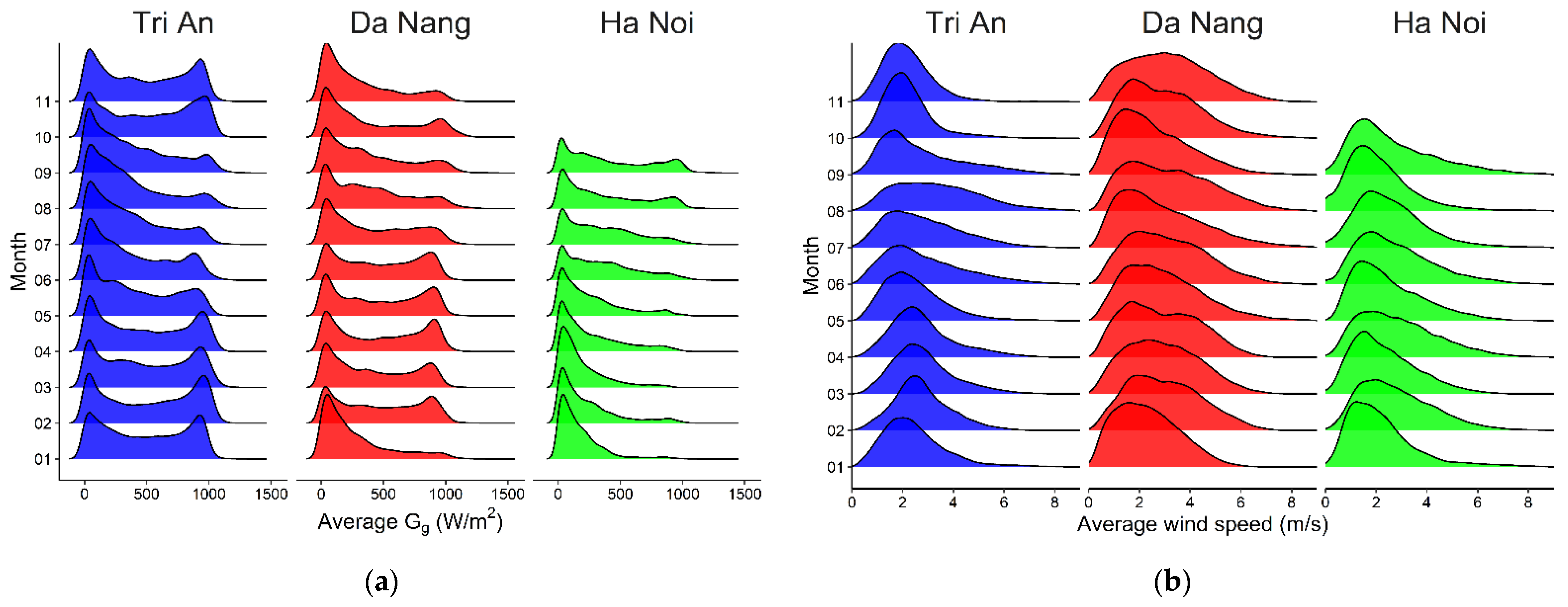
2.1. Data

Two databases were used for training and validating the proposed models. The first database was taken from ESMAP [20], which provide the measurements from different automated solar stations in Vietnam. Data for each site included one-minute averages of solar irradiance, PV module temperature, ambient temperature, and wind speed. Three data sets were selected from this database corresponding to three climatic zones in Vietnam: Hanoi in the north with subtropical with dry winter climate (Cwa), Danang in the center with equatorial monsoon climate (Am), and Tri An in the south with equatorial savannah with dry winter climate (Aw) [21]. The second database provides measured data for different PV modules in the USA, including crystalline silicon and thin film technologies, and is supplied by Marion [22]. Those modules were deployed in different locations: Cocoa, Florida, with subtropical climate; Eugene, Oregon, with marine west coast climate; and Golden, Colorado, with a semi-arid climate. Different from the former datasets, the data for these sites were measured immediately at a certain time of recording. The general characteristics of these databases are presented in Table 1.
The data in Group 1 were used for both training and validating the proposed models, while the data in Group 2 were used for evaluating the accurate prediction of those models on different PV module technologies compared to other literature models. The PV module technologies and their characteristics used in this study are presented in Table 2. Due to the lack of wind measurements, which needs to be measured on-site at the same conditions as other parameters, measurements of the wind speed at the 10-m height [24] and the nearest measured station [23] were applied.

2.2. Previous Models

There are many temperature models in the literature, so we have implemented and compared seven existing models presented in Table 3 with our proposed models in this study. In these selected models, some of them are able to predict the module temperature while others calculate the cell temperature directly. For the models predicting cell temperature, which becomes significantly different from the back-surface module temperature in high solar radiation intensities [3], the following relationship was applied:
T c = T m + G g G 0 · Δ T m ,
The temperature difference between the PV cell and module back surface was evaluated by King et al. [3] to be about ΔTm = 3 °C at an irradiance level of G g = G 0 for an open-rack installation PV system.
For the first Akhsassi model, the module efficiency and temperature coefficient of maximum power at STC were taken directly from the PVs’ characteristics. While the solar irradiance coefficient γ P m p is between 0.03 and 1.12 for silicon and most often simplified to γ P m p = 0 [10,11,25], it was chosen to be 0.04 in this study.

2.3. Selected Metrics for Evaluating the Methods

In order to evaluate the differences between the measured ( T m e a s u r e d ) and predicted ( T p r e d i c t e d ) operating temperature of the PV modules, three statistical metrics have been applied:
  • The correlation coefficient R2 defines the relationship between the estimated and measured data as the following expression:
    R 2 = ( i [ ( T p r e d i c t e d T ¯ p r e d i c t e d ) ( T m e a s u r e d T ¯ m e a s u r e d ) ] ) 2 i ( T p r e d i c t e d T ¯ p r e d i c t e d ) 2 ( T m e a s u r e d T ¯ m e a s u r e d ) 2 ,
  • The root mean square error, used to evaluate the fluctuations around the model and defined by the expression:
    R M S E = i n ( T m e a s u r e d T p r e d i c t e d ) 2 n ,

2.4. Proposed Models

2.4.1. Model with Wind

As mentioned above, several studies evidently showed that there is no best option, as we could not apply a unique temperature model for all PV module technologies. However, it was clear that the Sandia (King) model is frequently on the top list of matching temperature models. Besides, the Sandia model, unlike other temperature models, only takes on-site parameters such as plane-of-array (POA) irradiance, wind speed, and installation method into consideration. This reduction of input parameters leads to a simple implementation since it does not require many input parameters and a deep understanding of module technologies and materials.
As PV thermal models usually describe the module temperature based on the assumption of thermal equilibrium, the thermal mass of the module has a high impact on the responding time of the changes in the temperature [26]. Moreover, Segado et al. proved that the temperature prediction of a PV module is strongly affected by its own thermal inertia [9]. However, literature studies showed that Sandia is one of the models that is least affected by meteorological conditions. In other words, the changes in its empirical efficiencies are insignificant under different weather conditions and PV technologies [9,18,26]. Nevertheless, it was recognized that this model usually performed well under the low intensity of POA irradiance and less fluctuation of weather conditions; otherwise, it could suffer performance loss in practical implementation.
In this research, therefore, in order to improve the calculation of the module back-surface temperature, a modification of the Sandia model (Equation (2)) by adding a correction term was put forward, based on the idea of the relevance between module thermal inertia and interval sampling, presented by the following Equation:
T m = T a + Δ T r e f * G g G 0 E x p ( W s W r e f ) Δ T r e f Δ G g G 0 f ( Δ t ) ,
where Δ G g ( t ) = [ G g ( t ) G g ( t 1 ) ] is a dimensional constant describing the difference of POA irradiance between two consecutive sampling points ( Δ G g = 0   W / m 2 at t = 0 ); Δ t is the time recording interval in minutes; and Δ T r e f * and W r e f are empirical coefficients depending on module installation configuration and are equivalent to the coefficients a an b in the Sandia model from Ref. [3] and Equation (2). With Δ T r e f * = G 0 e a and W r e f = 1 b , this correction term becomes exactly the wind correction of Equation (2).

2.4.2. Model without Wind

As wind data are not always available for every PV system, there were many models without wind speed were presented to estimate the operating temperature of a PV cell/module. Some of them took into account the manufacturing and installing characteristics [15,27], while others neglected those parameters [11,14]. In this paper, we proposed a model based on the proportion of the POA irradiance to the solar irradiance at STC to calculate the operating temperature of a PV module without using wind velocity. At this suggestion, we assumed that the changing temperature of a PV module is proportional to the varying POA irradiance at operating conditions compared to the laboratory conditions. To improve the accuracy, the thermal mass of the PV module is once again taken into account, and our proposed model is expressed as the following Equation:
T m = T a + Δ T r e f * G g G 0 Δ T r e f Δ G g G 0 f ( Δ t ) ,

3. Results and Discussion

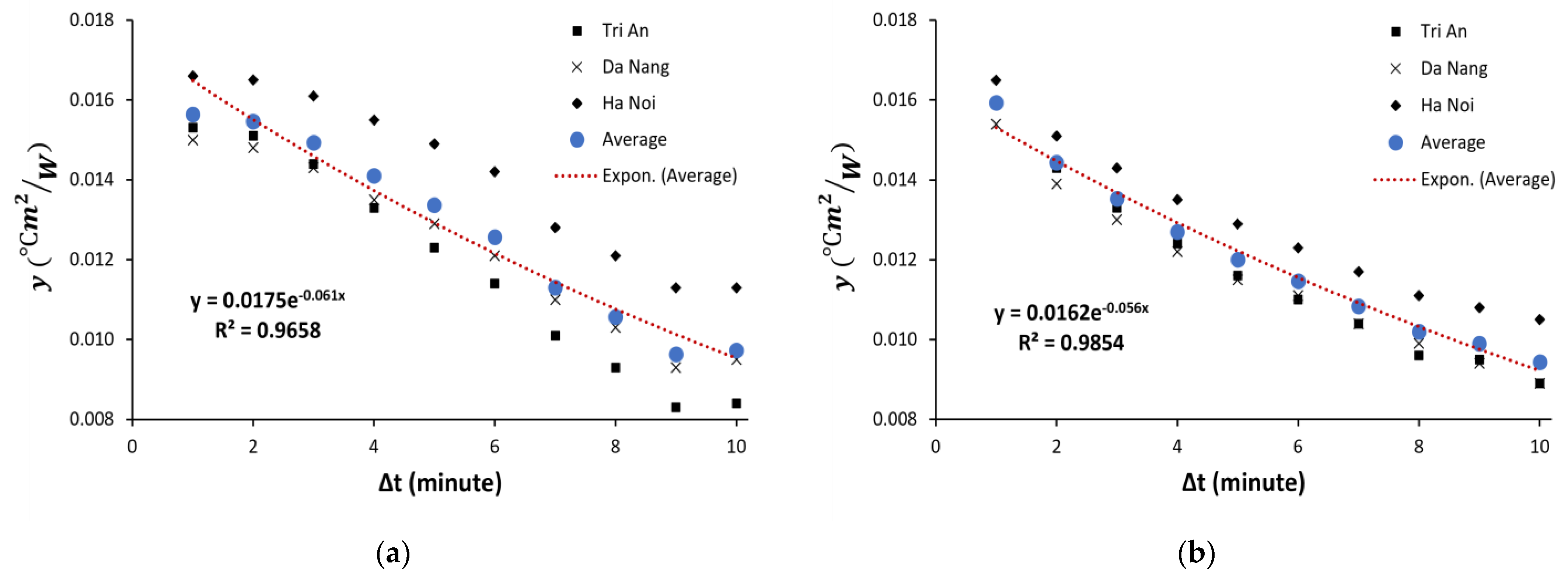
3.1. Parametric Identification

The measurements in 2018 from Group 1 in Table 1, which include POA irradiance, air temperature, wind speed, and module temperature, were selected to determine the coefficients of the suggested models. In these locations, the multi-crystalline silicon modules were installed with fixed open cracks; therefore, the coefficients Δ T r e f * and W r e f in Equation (11) were taken as 28.4 °C and 13.3   m / s , respectively. These values correspond with a = 3.56 and b = 0.075   s / m in the original Sandia model [3].
In the next stage, the best fit for the values y = Δ T r e f G 0 f ( Δ t ) , describing the relevance of the thermal inertia of the module and the interval sampling, were obtained as a function of the time step Δt for both models, based on measured data in three cities in 2018. The measurement data are available for every minute, and to determine y based on the time step Δ t , the measurement data of T m and Δ G g are averaged over the duration of the time step Δ t . The time step is limited to 10 min because otherwise, the time dependency is not described in sufficient detail. The resulting values of y and the corresponding correlation ( R 2 ) and error (RMSE) between the simulated values of the temperature T m and the measurement data for the proposed model with wind speed are presented in Table 4. The mean y ¯ , averaged over the three locations, and the related standard deviation (SD) were also calculated. The obtained values of y as a function of Δ t for both proposed models are illustrated in Figure 1. The relation between y ¯ and Δ t is approximately exponential and a least-squares fit yields R 2 equal to 0.97 and 0.99 for the model with wind speed and the model without wind speed, respectively: y ¯ = 0.0175 exp ( 0.061 Δ t ) and y ¯ = 0.0162 exp ( 0.056 Δ t ) . These relations can be used to eliminate the function ft) that we have introduced previously.
The Equation (11), therefore, becomes:
T m = T a + Δ T r e f * G g G 0 exp ( W s W r e f ) Δ T r e f Δ G g G 0 exp ( Δ t τ ) ,
where Δ T r e f = 18   ° C and τ = 16.7   min .
The same method was applied for the second model and then the Equation (12) becomes:
T m = T a + Δ T r e f * G g G 0 Δ T r e f Δ G g G 0 exp ( Δ t τ ) ,
with Δ T r e f * = T 0 = 25   ° C , Δ T r e f = 16   ° C and τ = 16.7   min .

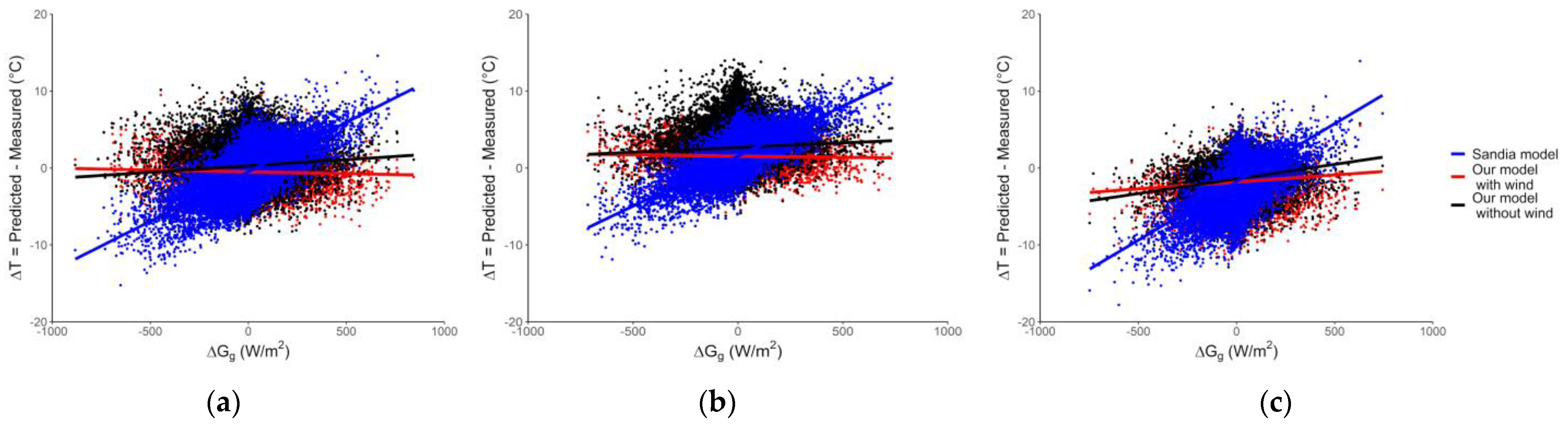
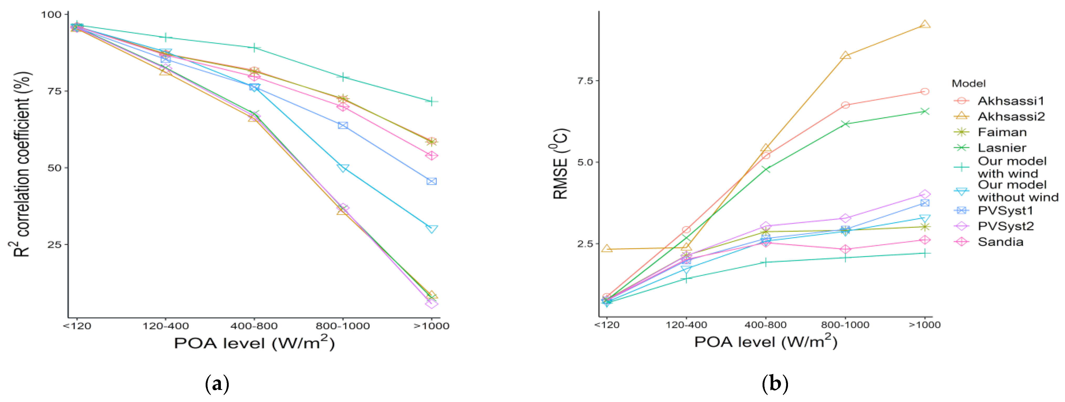
3.2. Models Comparison

At this stage, the recorded data in 2019 from three locations in Vietnam (Group 1 in Table 1) were taken out for evaluating the proposed models. After removing the samples which were recorded in the nighttime and all incorrect intervals, the total number of sampling points and corresponding time steps are presented in Table 5.
Besides comparing experimental measurements and model predictions, a comparison between proposed and literature models was also implemented and presented in Table A1 (see Appendix A). As was to be expected, our proposed model with wind presented the best correlation between calculations and measurements with R2 greater than 95% compared to other models, while the without-wind proposed model was the best in the group of models without wind speed. Moreover, the proposed model with wind illustrates that it has the most stable performance compared to all other models from the literature, as it is the only one that provided RMSE values less than 3   ° C for all regions. In contrast, the RMSE values for other models changed significantly between the three locations. Moreover, this method also obtained better results for both R 2 and R M S E coefficients at all time steps compared to the original Sandia model.
It was clear that the accuracy of all models was proportional to the interval time. As mentioned above, these models describe the temperature of PV modules under the assumption of their thermal equilibrium. Therefore, if this condition is not satisfied, then large differences can result. Moreover, it is known that the time response to changes in the temperature depends on the thermal mass of the module and the prevailing conditions [26], so that if the time resolution of the data is shorter than the typical thermal response times, the performance of the models will not be as good.
The difference between the predicted and measured values of the PV module back-surface temperature, Δ T , is illustrated in Figure 2. As we can see in the picture, the calculation for Sandia is proportional to the magnitude of fluctuating POA between two consecutive sampling points. The larger the variation, the greater the difference is. While the corresponding values for our proposed models tend to approach zero and are evenly distributed around zero across the range of Δ G g .
We also took into account the implementation of temperature models at different POA levels, which strongly affected the accuracy of the predicting process. The results displayed in Figure 3 demonstrate that the accuracy of the temperature models will decrease when the radiation intensity reaches the module surface increase. This circumstance occurred because the fluctuations among high POA values happen more frequently than those of low POA levels. Moreover, the greater POA the module gets, the higher the temperature of the module will be. Subsequently, the thermal inertia of the PV modules will have a stronger effect when POA increases, which explains why our proposed models perform better than literature models at high POA levels but remain equivalent when POA levels are low.
Figure 4 showed that the on-site wind speed of all regions remained stable during the observed period, while the average POA irradiance occurred in different ways. The POA irradiance in Tri An is distributed across the whole range of values, while the values of that parameter in Ha Noi are mainly concentrated below 500 W / m 2 . Moreover, Figure 4c illustrates that the distribution of the difference between two consecutive sampling points of wind is almost the same for all regions with variations between 0 and 3 m / s . While the largest fluctuation of POA irradiance occurred in Tri An, and the smallest fluctuation of that happened in Ha Noi. This means that the effect of thermal inertia on the thermal prediction in Tri An is greater than for the other regions due to its high intensity and frequent fluctuation of POA irradiance. Consequently, our proposed model with wind obtained the best result in Tri An where the on-site conditions fluctuated most significantly, while the proposed model without wind gained better performances in Tri An and Ha Noi, where the wind was less important than in Da Nang.
The back-surface temperature of the PV module that is calculated for three regions by our proposed model with wind effect (Equation (13)) using optimized values of Δ T r e f * and W r e f coefficients is presented in Table 6. By applying these best-fitted coefficients, the obtained R M S E values were decreased significantly to below 2 °C for all regions.

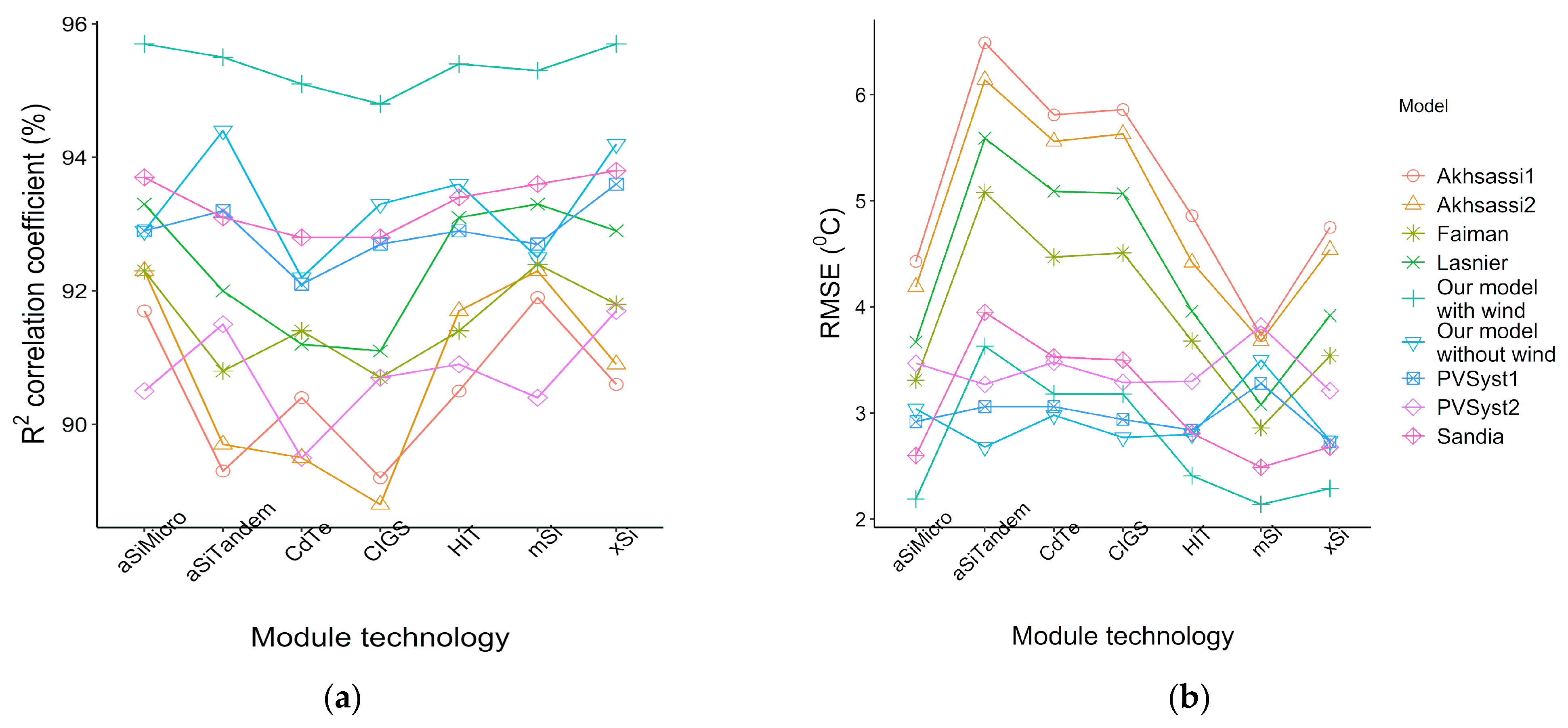
3.3. Comparison between Different PV Technologies

Our proposed models were examined afterwards with different module technologies, which were deployed in three locations in the USA. The obtained results for all regions are shown in Table A2 (see Appendix A), while a visual presentation for Cocoa is depicted in Figure 5. As we can see, our proposed model with wind obtained the best compatibility of predicting module temperature since it showed the highest correlation coefficient R2 and the lowest RMSE, whilst the other proposed model has the best performance among the models that ignore the influence of the wind, with highest R2 and lowest RMSE values calculated for all PV technologies and locations.
Previous studies have reported that it is difficult to apply a single model or a unique formula to precisely calculate the PV module/cell temperature [9,11,18,19]. Moreover, the thermal characteristics of PV modules are slightly different even if they are manufactured with the same technology and materials [12,13]. However, our proposed models have demonstrated that they can work well with different PV technologies and weather conditions without adjusting the empirical coefficients.
Table 7 shows the optimal coefficients, Δ T r e f * and W r e f in Equation (13), and corresponding implementing results which were calculated for various PV technologies in three different locations. As we can see, the operating temperature of CdTe and CIGS modules were least affected by on-site POA, with Δ T r e f * is 31.25 ± 0.45   ° C and 30.65 ± 0.75   ° C , respectively. Silicon PV module operating temperatures, on the other hand, were influenced significantly by local POA irradiance conditions, with Δ T r e f * equal to 28.6 ± 1.3   ° C and 27.65 ± 1.95   ° C , respectively, for xSi and mSi modules.

4. Conclusions

As the temperature has a significant effect on the electrical efficiency of solar cells, it is necessary to accurately estimate the photovoltaic module/cell temperature when predicting the energy yield. In this framework, we proposed two new models in order to calculate the PV module temperature. One model with the wind was developed based on the Sandia model by considering the effect of the thermal inertia of the module, whilst the other was determined without taking into account the wind speed. These proposed models have been compared to other models in the literature by using the statistical coefficients R 2 and R M S E . The results show that the inclusion of the thermal inertia of the PV module and the wind speed with the given models allow making a more accurate estimation of the module temperature, with R 2 correlation above 95% and the R M S E below 3 °C for most PV technologies.
As they do not need many input parameters and are simple to implement, these proposed models have demonstrated that they also work well under different environmental and operating conditions and PV technologies. The proposed model with wind, Equation (13), can be used to calculate PV module temperature with high precision for any location where wind data are available; otherwise, Equation (14) can be applied. These thermal models are useful for evaluating the thermal performance of a PV module under different environmental and operating conditions since they have proven their reliability when being examined in different locations and climates.
When climatological information such as wind speed and solar illumination are available in a time series for a certain location, our models make it possible to estimate the module temperature for different types of solar cells. The temperature information is essential in estimating the PV module efficiency and in deciding which kind of PV panel will be most economical for the given location.

Author Contributions

Conceptualization, D.P.N.N. and J.L.; Data curation, D.P.N.N.; Formal analysis, D.P.N.N.; Funding acquisition, J.L.; Investigation, D.P.N.N.; Methodology, D.P.N.N., K.N. and J.L.; Project administration, J.L.; Resources, K.N. and J.L.; Software, D.P.N.N.; Supervision, K.N. and J.L.; Validation, K.N. and J.L.; Writing—original draft, D.P.N.N.; Writing—review and editing, K.N. and J.L. All authors have read and agreed to the published version of the manuscript.

Funding

This research received no external funding.

Institutional Review Board Statement

Not applicable.

Informed Consent Statement

Not applicable.

Data availability Statement

Data available on request.

Conflicts of Interest

The authors declare no conflict of interest.

Nomenclature

T m Module temperature (°C)
T c Cell temperature (°C)
T a Ambient temperature (°C)
T 0 Reference temperature of 25 °C
η S T C Module efficiency coefficient (%)
β P m p Module temperature coefficient (%/°C)
G g Plane Of Array irradiance (POA) (W/m2)
G 0 Reference solar irradiance of 1000 W/m2
W s Wind speed (m/s)
U 0 The constant heat transfer component (W/m2K)
U 1 The convective heat transfer component (W/m3sK)
γ P m p Dimensionless coefficient between 0.03 and 0.12

Appendix A

Table A1. Results obtained for predicting module temperature with different time steps and models.
LocationModelR2 (%)RMSE (°C)
Time Step (Minutes)
151015151015
Tri AnSandia *94.396.197.097.52.452.061.841.72
Faiman *94.496.597.598.02.692.352.172.09
PVSyst1 *93.695.496.396.72.692.272.031.90
Akhsassi1 *94.596.597.497.84.554.464.424.41
Our model with wind *95.697.898.198.12.181.631.561.55
Lasnier92.593.894.494.74.194.084.034.01
PVSyst292.093.794.695.02.882.532.332.22
Akhsassi291.492.593.093.25.125.085.065.05
Our model without wind93.395.595.795.72.632.152.092.07
Da NangSandia *95.997.397.998.22.522.222.092.01
Faiman *95.296.997.698.02.201.821.641.55
PVSyst1 *95.496.797.397.63.633.413.313.26
Akhsassi1 *95.196.697.297.52.752.612.552.52
Our model with wind *96.798.598.798.82.351.951.881.87
Lasnier94.695.495.896.02.212.051.961.92
PVSyst294.195.395.896.13.823.633.543.50
Akhsassi293.694.294.594.63.213.143.103.07
Our model without wind95.096.496.596.53.723.493.463.46
Ha NoiSandia *96.397.297.797.93.062.892.802.75
Faiman *95.896.997.597.83.393.243.163.13
PVSyst1 *96.297.197.798.02.602.362.222.14
Akhsassi1 *94.995.896.396.54.914.894.874.87
Our model with wind *96.998.298.498.52.942.662.632.63
Lasnier93.794.294.594.74.844.804.784.77
PVSyst295.696.597.097.22.942.772.662.60
Akhsassi291.491.791.992.15.145.125.115.11
Our model without wind96.397.597.797.82.792.492.452.45
* Models with wind speed.
Table A2. The statistical coefficients (R2 and RMSE) for all models with and without wind speed vs. experimental measurement of module back-surface temperature calculated for different technologies.
CoefficientLocationModuleModel
With WindWithout Wind
SandiaFaimanPVSyst1Akhsassi1Our Model with WindLasnierPVSyst2Akhsassi2Our Model without Wind
R2
(%)
CocoaxSi93.891.893.690.695.792.991.790.994.2
mSi93.692.492.791.995.393.390.492.392.5
CdTe92.891.492.190.495.191.289.589.592.2
CIGS92.890.792.789.294.891.190.788.893.3
HIT93.491.492.990.595.493.190.991.793.6
aSiMicro93.792.392.991.795.793.390.592.392.9
aSiTandem93.190.893.289.395.592.091.589.794.4
GoldenxSi96.195.296.293.696.891.495.187.595.8
mSi95.994.596.392.896.891.795.687.796.5
CdTe95.494.595.692.896.590.994.787.195.7
CIGS95.094.594.893.196.190.393.486.894.4
HIT94.893.595.291.996.091.294.787.495.9
aSiMicro95.093.795.492.096.191.094.987.195.9
aSiTandem94.793.395.291.595.990.294.686.295.8
EugenexSi96.596.596.396.397.393.696.090.596.7
mSi96.896.696.596.897.695.596.593.097.3
CdTe95.995.895.695.896.893.695.490.896.3
CIGS95.595.595.295.496.492.995.090.195.8
HIT96.496.496.096.797.395.296.093.096.8
aSiMicro96.296.195.896.297.094.495.791.896.5
aSiTandem96.096.195.895.997.093.495.590.496.5
RMSE
(°C)
CocoaxSi2.683.542.734.752.293.923.214.542.74
mSi2.492.863.283.732.143.083.823.683.50
CdTe3.534.473.065.813.185.093.485.562.98
CIGS3.504.512.945.863.185.073.295.632.77
HIT2.813.682.844.862.413.963.304.422.80
aSiMicro2.603.312.924.432.193.673.474.193.04
aSiTandem3.955.083.066.493.635.593.276.142.68
GoldenxSi3.103.493.404.642.895.393.586.143.39
mSi3.233.992.945.432.956.143.126.702.80
CdTe3.574.323.075.883.286.873.427.173.08
CIGS3.333.633.634.773.015.693.906.253.63
HIT3.814.553.445.923.496.483.577.073.21
aSiMicro3.584.293.305.663.296.303.456.893.12
aSiTandem3.674.373.375.743.326.423.536.993.15
EugenexSi2.432.332.882.742.155.232.664.612.42
mSi2.422.353.072.322.174.572.613.922.40
CdTe2.702.692.943.342.415.882.875.012.60
CIGS2.732.683.093.132.475.592.944.842.70
HIT2.652.513.302.402.404.782.883.792.67
aSiMicro2.582.503.072.762.325.212.794.342.56
aSiTandem2.772.802.843.662.486.322.945.462.66

References

  1. IEA. Solar PV. IEA: Paris, France. Available online: https://www.iea.org/reports/solar-pv (accessed on 24 July 2021).
  2. Huld, T.; Gracia Amillo, A.M. Estimating PV module performance over large geographical regions: The role of irradiance, air temperature, wind speed and solar spectrum. Energies 2015, 8, 5159–5181. [Google Scholar] [CrossRef] [Green Version]
  3. Kratochvil, J.A.; Boyson, W.E.; King, D.L. Photovoltaic Array Performance Model; Albuquerque, N.M., Livermore, C.A., Eds.; MDPI: Basel, Switzerland, 2004; Volume 8. [Google Scholar]
  4. Cañete, C.; Carretero, J.; Sidrach-de-Cardona, M. Energy performance of different photovoltaic module technologies under outdoor conditions. Energy 2014, 65, 295–302. [Google Scholar] [CrossRef]
  5. Kurnik, J.; Jankovec, M.; Brecl, K.; Topic, M. Outdoor testing of PV module temperature and performance under different mounting and operational conditions. Sol. Energy Mater. Sol. Cells 2011, 95, 373–376. [Google Scholar] [CrossRef]
  6. Gaglia, A.G.; Lykoudis, S.; Argiriou, A.A.; Balaras, C.A.; Dialynas, E. Energy efficiency of PV panels under real outdoor conditions–An experimental assessment in Athens, Greece. Renew. Energy 2017, 101, 236–243. [Google Scholar] [CrossRef]
  7. Zsiborács, H.; Pintér, G.; Bai, A.; Popp, J.; Gabnai, Z.; Pályi, B.; Farkas, I.; Baranyai, N.H.; Gützer, C.; Trimmel, H.; et al. Comparison of thermal models for ground-mounted south-facing photovoltaic technologies: A practical case study. Energies 2018, 11, 1114. [Google Scholar] [CrossRef] [Green Version]
  8. Skoplaki, E.; Palyvos, J.A. Operating temperature of photovoltaic modules: A survey of pertinent correlations. Renew. Energy 2009, 34, 23–29. [Google Scholar] [CrossRef]
  9. Mora Segado, P.; Carretero, J.; Sidrach-de-Cardona, M. Models to predict the operating temperature of different photovoltaic modules in outdoor conditions. Prog. Photovolt. Res. Appl. 2015, 23, 1267–1282. [Google Scholar] [CrossRef]
  10. Mattei, M.; Notton, G.; Cristofari, C.; Muselli, M.; Poggi, P. Calculation of the polycrystalline PV module temperature using a simple method of energy balance. Renew. Energy 2006, 31, 553–567. [Google Scholar] [CrossRef]
  11. Akhsassi, M.; El Fathi, A.; Erraissi, N.; Aarich, N.; Bennouna, A.; Raoufi, M.; Outzourhit, A. Experimental investigation and modeling of the thermal behavior of a solar PV module. Sol. Energy Mater. Sol. Cells 2018, 180, 271–279. [Google Scholar] [CrossRef]
  12. Faiman, D. Assessing the outdoor operating temperature of photovoltaic modules. Prog. Photovolt. Res. Appl. 2008, 16, 307–315. [Google Scholar] [CrossRef]
  13. Koehl, M.; Heck, M.; Wiesmeier, S.; Wirth, J. Modeling of the nominal operating cell temperature based on outdoor weathering. Sol. Energy Mater. Sol. Cells 2011, 95, 1638–1646. [Google Scholar] [CrossRef]
  14. Soteris, A. Kalogirou Solar Energy Engineering: Processes and Systems; Elsevier Inc.: Amsterdam, The Netherlands, 2009; ISBN 9780123745019. [Google Scholar]
  15. PVsyst 7 Help, Array Thermal Losses. Available online: https://www.pvsyst.com/help/index.html (accessed on 18 March 2021).
  16. Skoplaki, E.; Boudouvis, A.G.; Palyvos, J.A. A simple correlation for the operating temperature of photovoltaic modules of arbitrary mounting. Sol. Energy Mater. Sol. Cells 2008, 92, 1393–1402. [Google Scholar] [CrossRef]
  17. Muller, M.; Marion, B.; Rodriguez, J. Evaluating the IEC 61215 Ed.3 NMOT procedure against the existing NOCT procedure with PV modules in a side-by-side configuration. In Proceedings of the 2012 38th IEEE Photovoltaic Specialists Conference, Austin, TX, USA, 3–8 June 2012; pp. 697–702. [Google Scholar] [CrossRef]
  18. Zouine, M.; Akhsassi, M.; Erraissi, N.; Aarich, N.; Bennouna, A.; Raoufi, M.; Outzourhit, A. Mathematical models calculating PV module temperature using weather data: Experimental study. Lect. Notes Electr. Eng. 2019, 519, 630–639. [Google Scholar] [CrossRef]
  19. Schwingshackl, C.; Petitta, M.; Wagner, J.E.; Belluardo, G.; Moser, D.; Castelli, M.; Zebisch, M.; Tetzlaff, A. Wind effect on PV module temperature: Analysis of different techniques for an accurate estimation. Energy Procedia 2013, 40, 77–86. [Google Scholar] [CrossRef] [Green Version]
  20. Vietnam—Solar Radiation Measurement Data obtained from World Bank via ENERGYDATA.info. Available online: https://energydata.info/dataset/vietnam-solar-radiation-measurement-data (accessed on 11 April 2021).
  21. Polo, J.; Gastón, M.; Vindel, J.M.; Pagola, I. Spatial variability and clustering of global solar irradiation in Vietnam from sunshine duration measurements. Renew. Sustain. Energy Rev. 2015, 42, 1326–1334. [Google Scholar] [CrossRef]
  22. Marion, B.; Anderberg, A.; Deline, C.; Del Cueto, J.; Muller, M.; Perrin, G.; Rodriguez, J.; Rummel, S.; Silverman, T.J.; Vignola, F.; et al. New data set for validating PV module performance models. In Proceedings of the 2014 IEEE 40th Photovoltaic Specialist Conference, Denver, CO, USA, 8–13 June 2014; pp. 1362–1366. [Google Scholar] [CrossRef]
  23. Lustbader, J.; Afshin, A. NREL Vehicle Testing and Integration Facility (VTIF): Rotating Shadowband Radiometer (RSR). Golden, Colorado (Data); NREL Report No. DA-5500-56490. Available online: https://midcdmz.nrel.gov/apps/sitehome.pl?site=VTIF (accessed on 26 April 2021).
  24. Global Modeling and Assimilation Office (GMAO). MERRA-2 tavg1_2d_slv_Nx: 2d,1-Hourly, Time-Averaged, Single-Level, Assimilation, Single-Level Diagnostics V5.12.4. Goddard Earth Sciences Data and Information Services Center (GES DISC): Greenbelt, MD, USA, 2015. Available online: https://goldsmr4.gesdisc.eosdis.nasa.gov/data/MERRA2/M2T1NXSLV.5.12.4/ (accessed on 27 January 2021).
  25. Evans, D.L. Simplified method for predicting photovoltaic array output. Sol. Energy 1981, 27, 555–560. [Google Scholar] [CrossRef]
  26. Armstrong, S.; Hurley, W.G. A thermal model for photovoltaic panels under varying atmospheric conditions. Appl. Therm. Eng. 2010, 30, 1488–1495. [Google Scholar] [CrossRef]
  27. Ross, R.G. Interface design considerations for terrestrial solar cell modules. In Proceedings of the 12th Photovoltaic Specialists Conference, Baton Rouge, LA, USA, 15–18 November 1976; pp. 801–806. [Google Scholar]
Figure 1. Plot of the values of y = Δ T r e f G 0 f ( Δ t ) in different time steps from Table 4 and exponential fitting curve for the mean value y ¯ . (a) Model with wind speed. (b) Model without wind speed.
Applsci 11 07064 g001
Figure 2. A comparison of the difference between predicted and measured temperature of PV module in three different locations, resulting in changing of incident POA with 5-min time steps: (a) Tri An; (b) Da Nang; and (c) Ha Noi.
Applsci 11 07064 g002
Figure 3. Correlation between measured and calculated module temperature for different POA levels obtained with the studied models for Tri An, Vietnam (time recording = 5 min): (a) correlation factor R 2 ; (b) R M S E .
Applsci 11 07064 g003
Figure 4. The distribution of POA irradiation and wind in three locations in Vietnam (1-min time step): (a) average monthly distribution of POA irradiation level; (b) average monthly distribution of wind speed; and (c) the variation of POA irradiance and wind speed between two consecutive sampling points.
Applsci 11 07064 g004aApplsci 11 07064 g004b
Figure 5. Correlation between measured and calculated module temperature for different module technologies obtained with the studied models for Cocoa, USA: (a) correlation factor R2; (b) RMSE.
Applsci 11 07064 g005
Table 1. Selected databases for training and validating models.
GroupLocationLatitude
N)
Interval Sampling
(Minute)
Observed Period
1Tri An 111.01101/2018–11/2019
Da Nang 116.01101/2018–11/2019
Ha Noi 121.20101/2018–09/2019
2Cocoa 228.39501/2011–03/2012
Golden 239.741508/2012–09/2013
Eugene 244.05510/2012–01/2014
1 Selected data from [20]. 2 Selected data from [22,23,24].
Table 2. Technologies and main characteristics of the different modules.
Module TechnologyCharacteristicsSampling Points
ηSTC (%) β P m p ( % ° C ) CocoaGoldenEugene
Single-crystalline silicon (xSi) 113.60−0.4229,63210,26637,820
Multi-crystalline silicon (mSi) 214.00−0.4128,24810,26838,016
Cadmium telluride (CdTe) 18.85−0.2129,73010,36237,062
Copper indium gallium selenide (CIGS) 111.2−0.3929,71410,40537,815
Amorphous silicon/crystalline silicon (HIT) 117.6−0.3529,11910,29237,985
Amorphous silicon/microcrystalline silicon (aSiMicro) 17.5−0.3629,70110,57838,022
Amorphous silicon tandem junction (aSiTandem) 14.47−0.2529,85310,41337,970
1 Deployed in Cocoa, Golden and Eugene. 2 Deployed in Cocoa, Golden, Eugene, Tri An, Da Nang and Ha Noi.
Table 3. Literature models for validating proposed models.
GroupsCorrelationsCommentsRef.Equation
With windSandia: T m = T a + G g exp ( a + b W s ) a = 3.56
b = 0.075   s / m
[3](2)
Faiman: T m = T a + G g U 0 + U 1 W s     U 0 = 30.2   W / m 2 / ° C
U 1 = 6.28   Ws / m 3 / ° C
[12,13](3)
PVSyst1: T c = T a + G g ( 1 η m ) U 0 + U 1 W s U 0 = 25   W / m 2 / ° C
U 1 = 1.2   Ws / m 3 / ° C
α = 0.9 ,   η m = 0.1
[15](4)
Akhsassi1:
T m = U L T a + [ ( τ α ) η S T C ( 1 β P m p T 0 ) ( 1 + γ P m p L n ( G g G 0 ) ) ] G g U L + η S T C β P m p ( 1 + γ P m p L n ( G g G 0 ) ) G g
U L = U 0 + U 1 W s
U 0 = 24.68   W / m 2 / ° C
U 1 = 6.13   Ws / m 3 / ° C
[11](5)
Without windLasnier: T m = 30   ° C + 0.0175   ° C m 2 W ( G g 300 W m 2 ) + 1.14 ( T a 25   ° C ) [14](6)
PVSyst2: T c = T a + G g ( 1 η m ) U 0 + U 1 W s    U 0 = 29   W / m 2 / ° C
   U 1 = 0   Ws / m 3 / ° C
α = 0.9 ,   η m = 0.1
[15](7)
Akhsassi2: T m = 25   ° C + 0.123   ° C m 2 W ( G g 200   W / m 2 ) + 1.04 ( T a 20   ° C ) [11](8)
Table 4. Calculated values of y = Δ T r e f G 0 f ( Δ t ) , correlation (R2), and error (RMSE) between measured and simulated temperature Tm for three cities and for different values of the time step Δt.
Time Step
(Min.)
LocationAverage
Tri AnDa NangHa Noi
y ( ° C   m 2 W )
R2
(%)
RMSE
(°C)
y ( ° C   m 2 W )
R2
(%)
RMSE
(°C)
y ( ° C   m 2 W )
R2
(%)
RMSE
(°C)
y ¯ ( ° C   m 2 W )
SD
10.015391.42.810.015093.62.730.016693.73.830.01560.00085
20.015193.52.570.014895.22.510.016595.13.660.01550.00091
30.014494.62.430.014396.22.370.016195.93.560.01490.00101
40.013395.22.350.013596.72.290.015596.43.500.01410.00122
50.012395.52.320.012996.72.240.014996.73.460.01340.00136
60.011495.72.300.012197.22.210.014296.93.450.01260.00146
70.010195.72.300.011097.22.200.012896.93.450.01130.00137
80.009395.72.300.010397.32.190.012197.03.440.01060.00142
90.008395.72.310.009397.32.190.011397.13.450.00960.00153
100.008495.82.290.009597.42.170.011397.23.440.00970.00146
Table 5. The sample size of measurements in different time steps for three regions in Vietnam.
Time Step
(Minute)
Sampling Point
Tri AnDa NangHa Noi
1246,982247,703198,476
549,40149,54239,703
1024,39524,46719,597
1516,13616,18712,975
Table 6. Correlation coefficients ( R 2 and R M S E ) for measured and calculated module temperatures for three regions in Vietnam using optimal coefficients (5-min time step).
CoefficientsImplementing Results
Tri AnDa NangHa Noi
Δ T r e f *
(°C)
31.424.734.7
Wref (m/s)11.111.812.8
R2 (%)98.098.498.4
RMSE (°C)1.431.401.55
Table 7. Correlation coefficient R 2 and R M S E between measured and calculated module temperatures for different PV technologies using optimal coefficients.
PV TechnologyImplementing Results
CocoaGoldenEugenea
Δ T r e f * ( ° C )
Wref
(m/s)
R2
(%)
RMSE
(°C)
Δ T r e f * ( ° C )
Wref
(m/s)
R2
(%)
RMSE
(°C)
Δ T r e f * ( ° C )
Wref
(m/s)
R2
(%)
RMSE
(°C)
xSi27.321.796.22.0029.912.297.02.8629.68.397.42.04
mSi25.718.595.52.0529.618.997.32.5427.39.797.71.86
CdTe30.817.594.92.4731.715.297.02.5430.88.596.92.37
CIGS29.920.895.22.3731.410.196.32.9330.28.396.42.41
HIT27.322.295.82.1029.621.396.53.0227.98.397.52.02
aSiMicro27.119.695.82.0629.618.996.62.9029.08.597.12.19
aSiTandem31.122.295.92.2729.619.296.52.9131.78.897.02.38
Publisher’s Note: MDPI stays neutral with regard to jurisdictional claims in published maps and institutional affiliations.

