Abstract
The paper deals with the reliability-centered maintenance (RCM) of a transmission substation. The process of the planning and actual performance of maintenance was carried out using an optimization algorithm. This maintenance procedure represents the maintenance management and included reliability of the power system operation, maintenance costs, and associated risks. The originality of the paper lies in the integrated treatment of all maintenance processes that are included in the pre-processing and used in the optimization process for reliability-centered maintenance. The optimization algorithm of transmission substation maintenance was tested in practice on the equipment and components of an existing 400/110–220/110 kV substation in the Slovenian electricity transmission system. A comparison analysis was also carried out of the past time-based maintenance (TBM) and the new reliability-centered maintenance (RCM), on the basis of the optimization algorithm.
1. Introduction
Maintenance is a combination of technical, administrative, and managerial actions during the lifetime of a device, the purpose of which is to keep it in, or bring it back to, the condition that enables performing of its functions. It is, therefore, a usual process needed by every device for normal operation. The maintenance in transmission substations (TS) is crucial for secure and reliable operation of the electric power system (EPS). The maintenance terminology covers two types of maintenance: preventive and corrective. In the field of electricity transmission devices, preventive maintenance still prevails [1]. This type of maintenance can be either time-based maintenance or related to the state of devices, condition-based maintenance (CBM) [2]. From 2009 onwards, the health index [3,4,5] has been used in the field of condition-based maintenance to evaluate indicators of maintenance.
However, new trends in the field of maintenance, i.e., reliability -centered maintenance (RCM), are being introduced in the wider area of engineering [6,7], as well as in the field of maintenance of devices in the electricity transmission system [1,8,9,10]. These trends are also accelerated by the standardization in the field of maintenance and asset management [11,12].
The reliability of operation and associated maintenance is, in the majority of cases, based on the reliability calculation using the Markov model [9,13,14,15]. An adequate efficiency of the determination of system criteria for maintenance can be achieved with the selection of various algorithms, such as the best–worst method (BWM) [16], where numerous possibilities are assessed on the basis of determination with regard to various attributes, and the best maintenance criteria are selected.
In the maintenance process, authors have also included optimization procedures dealing with economy and reliability [10,17,18,19]. The authors usually deal with individual elements, such as overhead lines [5,20] and transformers [21,22]. References [9,23] deal with maintenance of devices in a TS. The authors describe a maintenance method that is based on the technical condition of the devices. Certain authors have also investigated time scheduling of maintenance tasks [14,24] or determination of the optimal inspection interval of equipment in the TS, taking into account its age [25]. The authors of the presented paper, in [26], discussed the strategic maintenance of switching substations where reliability indices were not optimized.
The contribution of this paper is in the calculations of reliability indicators using the failure effect analysis (FEA) method, and not with the calculations of Markov chains for an individual device. In this method, any change in the state of an individual device affects the entire TS, which can, consequently, change the state of other devices as well. The maintenance processes of the devices in the substation are closely related to the reliability indicators (one of them is importance) for the entire TS, and, at the same time, to the condition of the individual devices, which is one of the article’s contributions.
The novelty presented in the present paper lies in the integrated treatment of TS maintenance based on the RCM concept, using an optimization algorithm. The modified differential evolution optimization algorithm with self-adaptation (SA) of the control parameters was used to select the optimal maintenance period of TS devices (revisions are carried out every year, every two years, or every three years), while the maintenance is carried out when the significant operational state of the EPS is the most suitable for it. This state is defined by generation, consumption, and power flows in the EPS. The method of EPS elements’ maintenance used until now is TBM, where their maintenance periods are defined by the TSO’s internal rules. The main objective of this approach is to reduce maintenance costs while keeping the operational reliability level and improving the maintenance system constantly. This procedure is possible only with the inclusion of optimization algorithms in the maintenance process. Devices that are less important in the system, however, affect maintenance processes with reduced intensity.
The maintenance processes can be influenced by computation of the importance and technical condition of EPS elements, which is based on historical data of operation, events, and monitoring of EPS elements’ technical condition. This represents the main hypothesis of this article. The inclusion of optimization processes in the analysis of maintenance procedures enables a reduction of maintenance costs, which represents the second hypothesis.
The methodology of computation of frequency of EPS elements’ maintenance influences the maintenance processes and is based on available historical operation data and statistics of events on EPS elements. For the entire EPS, we computed the availability of elements in connection with the transmissioned energy. The availability of elements and transmissioned energy to final customers are reliability indicators. The values of these indicators for individual elements were then compared with the reliability indicators of similar elements operated by other system operators. The importance of elements were computed on the basis of these data. In connection with the technical conditions of elements that are performed in practice through monitoring, it is possible to influence the maintenance processes on the basis of the RCM maintenance concept.
The optimization process that uses all possible data on historical events of operation and maintenance costs yields the results that can be used to manage the maintenance processes in the future. This represents the main originality of this paper. The existing method of assessing the technical condition of EPS elements was upgraded and included actively in the optimization process, where we predicted a dynamic changing of the technical condition of elements due to the interventions to the existing maintenance process.
The significant states in the system are determined on the basis of EPS operation data that include generation, nodal loads, and load flows between the nodes. Their inclusion in the optimization process enables that maintenance activities are performed in the most suitable significant state. Thus, the maintenance activities have the least impact on the EPS operation. Indirectly, this also influences operational reliability and maintenance costs. The optimization process in our article affects the frequency of transitions between maintenance processes.
The past data on the operation of transmission elements that are covered by statistics of events were the basis for calculation of reliability indicators of these elements and their unavailability. The values of these indicators for individual elements were compared with reliability indicators of similar elements operated by other system operators.
The paper consists of six sections. Section 2 presents the RCM concept-based maintenance model. A switching bay was represented with an index of technical condition and an index of importance. The costs of the existing maintenance concept were analyzed in detail. Section 3 provides the basic data for the optimization model. The key data in the RCM maintenance process were the values of technical condition and reliability indicators for every EPS element. The data are also given on the expected costs of outages and maintenance costs for the example presented in this article. Section 4 presents the link between the maintenance model and the optimization algorithm. Three objective functions and one penalty function were defined to reach the optimal RCM maintenance concept. The results of the optimization process are given in Section 5. The optimal method and period of maintenance were defined accurately for each EPS element. A comparison was also given of maintenance costs with the existing time-based maintenance and with the new RCM maintenance concept. Section 6 provides the discussion and outlines the future work.
2. Maintenance Model Based on the RCM Concept
RCM is a maintenance concept that, in addition to the basic maintenance methodologies, is focused on reliability. The objective of the RCM concept is management of maintenance costs and associated risks, having in mind the provision of adequate reliability of operation of the EPS. It is important not to treat reliability at the level of individual elements, but at the level of the entire system. Maintenance tasks carried out during maintenance are as follows: periodical inspection of elements performed on the energized state of the equipment; revision intended to retain elements’ functionality, performed on the de-energized state of equipment; and repair or replacement of elements. Elements with lower importance and good technical condition are maintained in the RCM concept using TBM in a longer time period. The main aim of RCM in this paper was to determine the maintenance periods of EPS elements with regard to their importance and condition, considering reliability and costs. This is the main change with regard to the TBM concept, where maintenance periods are determined in advance. The RCM concept in the paper is based on [1], while the basic concept uses the standard [11].
Section 2 is dedicated entirely to the RCM concept and consists of seven subsections. The elements are defined in Section 2.1 EPS. This includes a general set of elements and the term switching bay. The structure of the model of input data for optimization in the maintenance process is presented in Section 2.2. Since we wished to include ecology in the optimization process, Section 2.3 defines the characteristic variable of diagnostics of drops in pressure of the SF6 insulation gas. One of the key parameters in the RCM process is the index of technical condition. For each type of EPS element, there is a methodology for assessing their technical condition, which is described in Section 2.4. The next key parameter in the RCM concept is the index of importance of an EPS element, which is described in detail in Section 2.5. The cost-related part of our concept is dealt with in Section 2.6 and Section 2.7.
2.1. Definition of EPS Elements
The subject of our analyses is the EPS. It comprises generation units, lines, and substations. In substations, there are disconnectors, circuit breakers, power transformers, and other elements. The elements of the EPS represent a set of elements Sel = {elk; 1 ≤ k ≤ nel; k ∈ N}, where nel is the number of elements in the entire EPS, el is the element in the EPS, and k is the counter of the EPS elements. All these elements form a database with characteristic variables, such as estimation of technical condition, economic indicators, reliability indicators, and indicator of importance. A set of elements Skel = {kelr; 1 ≤ r ≤ nkel; r ∈ N} is created, where nkel is the number of kinds of elements used in the EPS, kel is the kind of elements used in the EPS, and r is the counter of kinds of elements used in the EPS. Data on the entire EPS are needed for the computation of the reliability indicators of the EPS, technical condition of elements, and maintenance costs. From the set of elements Sel, only those elements were observed that are a part of the TS.
The model enables scheduling of maintenance tasks with regard to the state of the system, taking into consideration economic effects and reliability of operation of individual switching bays in the TS.
The analysis includes only switching bays and transformers that are elements of the observed TS. A switching bay is a set of elements in the substation that belongs to the main element (transformer or transmission line). A switching bay is an assembly of switchgear elements (disconnectors, circuit breakers, etc.), and can be either line bay, transformer bay, or bus coupler bay [27]. Bays in the TS form a set of bays SSB = {SSB,l; SSB,l ⊂ Sel; 1 ≤ l ≤ nSB; l ∈ N}, where nSB is the number of switching bays. The lth bay in the TS comprises a certain number of elements and forms the set of elements of the lth bay SSB,l = {elSB,lm; 1 ≤ m ≤ nSB,l; m∈N}, being a subset of the set of elements Sel, where nSB,l is the number of elements in the lth bay of the TS and m is the counter of elements in the TS bay. A switching bay can be considered as a new EPS element. The reason for this is that, during revision, the entire bay is always in a de-energized state and is maintained as a whole. The analysis of a TS also includes power transformers. The set of bays in the TS is, thus, case extended to the number of transformers nT. It is defined as ST = {TRll; 1 ≤ ll ≤ nT; ll ∈ N}, where ll is the counter of transformers in the TS. The set of TS elements, therefore, consists of switching bays and transformers, and is defined as SSU = {SSU,q; SSU = SSB ∪ ST; 1 ≤ q ≤ nSU; q∈N; nSU = nSB + nT}, where q is the counter of switching bays and transformers and nSU is the number of observed switching bays and transformers of the TS.
2.2. The Structure of the Model
Figure 1 shows a block diagram of the preparation of input data for the optimization of maintenance tasks in transmission substations.
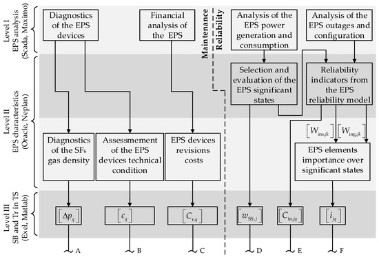
Figure 1.
Block diagram of the RCM concept-based maintenance model.
The following data are needed for this optimization: drop in pressure of SF6 in circuit breakers (CB), estimation of the technical condition of substation elements, financial data on switching bays’ maintenance, and reliability indicators for elements of switching bays and transformers.
2.3. Diagnostics of the Density of SF6 Gas
Diagnostics of the EPS devices is performed as a part of regular maintenance activities of EPS elements, and includes inspections, measurements, etc. One of the tasks of diagnostic activities are measurements of drops in pressure Δp of the SF6 insulation gas in circuit breakers. Circuit breakers in the switching bays are a part of the set of all SF6 circuit breakers in the EPS: SSF6 = {CBSF6,kk; CBSF6,kk ⊂ Sel; 1 ≤ kk ≤ nSF6; kk ∈ N}. The characteristic variable of the set of circuit breakers SSF6 is the vector of drop in pressure in the SF6 circuit breakers ΔpSF6 = [Δpkk], where kk is the counter of SF6 circuit breakers and nSF6 is the number of SF6 circuit breakers in the TS.
If there is an SF6 circuit breaker in the lth bay (e.g., the kkth element), the drop in pressure Δpkk can be considered as the characteristic variable of this element. In this case, we can write Δpl = Δpkk, otherwise Δpl = 0. All the bays in the TS form a vector of drops in pressure in circuit breakers ΔpSB = [ΔpSB,l]. The vector of drops in pressure of SF6 for all TS elements is, thus, defined as Δp = [Δpq], where Δpq = ΔpSB,l for 1 ≤ q ≤ nSB, l = q and Δpq = ΔpT,ll = 0 for nSB + 1 ≤ q ≤ nSB + nT and ll = q − nSB. These are the input data for the optimization procedure.
2.4. Index of Technical Condition c
Diagnostics of the EPS devices are also the basis for estimation of the technical condition of the EPS devices. For each kind of EPS element, there is an adopted methodology for estimation of the technical condition of devices ck [26]. The index of the technical condition is determined on the basis of the Slovenian transmission system operator internal application for determination of technical condition ck, which contains a set of 18 criteria with an adequate weighting factor (from 1 to 10), and each rating factor (from 1—good to 10—bad). The rating factor is determined by the engineer responsible for monitoring the switching substation for each corresponding criterion of the element.
The values of the technical condition of an element can lie in the range 0 ≤ ck ≤ 100. The higher the value is, the worse the technical condition of the EPS element. The technical condition of all EPS elements is evaluated in this way and is included in cs = [ck]. The lth switching bay of the TS contains a certain number of elements nSB,l and forms the set of elements of this bay. The characteristic variable of the set SSB,l is the vector of technical condition of the elements of this set, which is defined as cSB,l = [cSB,lm]. The technical condition cl of the lth bay can be defined as the maximum estimated value of technical condition of this bay’s elements, i.e., as cl = max(cSB,l). The vector cSB = [cl] can be defined for all the bays in the substation. The values of technical condition for power transformers are defined as cT = [cT,ll]. The vector of technical condition for the entire TS, including both bays and transformers, c = [cq], is obtained using the identical procedure, as described in Section 2.3.
2.5. Index of Importance i
To calculate the importance of the EPS elements, the reliability indicators need to be calculated first. The first step in this calculation is a detailed analysis of the EPS as a whole. For the calculation of reliability indicators, we used a powerful program tool for steady-state calculations in the EPS, Neplan [26]. The Neplan program tool for calculation of reliability indicators requires data on outages of all EPS elements, as well as hourly data on generation and consumption for all EPS nodes. The analysis begins with a statistical survey of hourly data on generation and consumption in all EPS nodes, as well as an analysis of power flows in certain parts of the EPS in a certain period (one year or more). A clustering approach is used on the basis of historical data. Average values of power (μP) and deviations from the average value (σP) are calculated for generation, consumption, and power flows. Combinations of strings of hourly data for the total power PSYS are selected, which is defined as the total power of generation, consumption, and power flows for the entire EPS. The nSS sets of significant states (SS) are selected for generation, consumption, and power flows for the combinations that appear most often. SS are states in the EPS with a certain quantity of generation, load flows, and consumption. Significant states are each a static snapshot that combines generation, consumption, and transmission. SS can be a variable (SS).
SSS = {hSS,j; 1 ≤ j ≤ nSS; j ∈ N}, where hSS,j is the characteristic hour from the selected jth set of states. Table 1 presents 9 selected SS for generation, consumption, and power flows that, to a certain extent, reflect the state of the EPS in the observed period. This is important in deciding when to implement maintenance of the TS elements.

Table 1.
Selected significant states for EPS.
It is also possible to calculate the shares of frequency of occurrence of SS that are characterized by generation and consumption in the selected hours of the observed period. Thus, the vector of shares of selected states in the EPS wSS = [wSS,j]; 0 < wSS,j < 1 is calculated (Table 1). The weight wSS,j depends on the share of hours in an individual set SSS,j of the whole set of hours.
For a certain past period, the data on outages of EPS elements are collected and modified in the reliability model of the Neplan program tool. In the model, it is also necessary to make possible changes of the EPS configuration. For each chosen jth SS reliability indicators are calculated in Neplan using the failure effect analysis (FEA) [28]. For the subsequent calculations, the costs are used of expected long duration outages of the EPS elements. The data on energy not supplied to the consumers Wins,jk in the case of an outage of a certain EPS element are included in the matrix wins = [wins,jk], while the matrix wing = [wing,jk] contains data on energy not produced in the generation units Wing,jk. Wins,jk and Wing,jk for every significant state and every certain element of EPS are calculated with FEA in the program tool Neplan. They are reliability indicators.
For each element r from the set of elements Sel, the subset Sel,jrv is created for each significant state j, kind of elements r, and a certain voltage level v Sel,jrv = {Wins,jkrv, Wing,jkrv; 1 ≤ k ≤ nkel; 1 ≤ v ≤ 3; k, v ∈ N}. For each significant state j and kind of elements r, Winmax,rv is determined, which is the maximum value from the set Sel,jrv, and for a certain voltage level v from the set SVL; SVL = {110 kV, 220 kV, 400 kV}. On the basis of these data, we are able to calculate the importance of the kth EPS element for the jth SS using kind of element r, and certain voltage level v is calculated as
which is based on experiences of the transmission system operator (TSO) ELES, and foresees that energy not supplied contributes 80% to the importance, while energy not produced contributes the remaining 20%, where v is a counter of voltage levels between 1 ≤ v ≤ 3. Thus, the matrix of importance ISSEPS = [ijk] is determined for all SS and the entire EPS.
The matrix of importance for the lth switching bay of the TS can be created for all significant states as ISB,l = [iSB,ljm]. From the matrix ISB,l for the jth SS, the vector iSB,jl = [iSB,jlm]; 1 ≤ m ≤ nSB,l is created, and, for the jth SS, the total importance of the lth bay is determined using the equation ijl = max(iSB,jl). From these vectors, the matrix of importance for all significant states ISB = [ijl] is created for all TS bays. In a similar way, the matrix of importance is created for power transformers in the TS IT = [iT,jll]. The total importance of all TS elements is obtained by joining the matrices ISB and IT to I = [ijq], where ijq = iSB,jl for 1 ≤ j ≤ nSS, 1 ≤ q ≤ nSB and l = q, and ijq = iT,jll for 1 ≤ j ≤ nSS and nSB + 1 ≤ q ≤ nSB + nT, and ll = q − nSB.
2.6. Past Maintenance Cost
It is necessary to perform a detailed financial analysis of the entire EPS for the determination of maintenance costs, which includes analysis of incomes, maintenance costs, and replacements of TS elements. This analysis is carried out by a unified information system (IBM Maximo). From the database, it is possible to obtain revision costs for all EPS elements CrEPS = [Cr,k] for the past period in EUR/year. For the lth bay of the TS, it is possible to create the vector of revision costs, defined as CrSB,l = [CrSB,lm]. The total annual revision costs for the lth bay are defined as the sum of costs for all its elements:
Using (2), the vector is obtained of all revision costs by switching bays CrSB = [Cr,l]. The vector of revision costs for power transformers CrT = [CrT,ll] is obtained in a similar way. The total revision costs for all TS elements Cr are obtained using the above-described procedure for determination of the vector Δp.
2.7. Expected Costs of Outages
The computation of the reliability model in the Neplan program tool yields as the final result FEA for each element k and each SS j the total anticipated costs of outage of all consumers by power CinP,jk in EUR/year, caused by an outage of the element k in SS j (which are affected by outage of the element k in SS j). The expected costs depend on individual contracts between the TSO and each consumer, the power of consumption, and the duration of each customer’s outage that is affected by an outage of element k in SS j. Following the FEA procedure, the maximum value of reliability indicators is obtained as a result. This method captures all possible changes in the state of devices in the TS.
The scaled costs of total energy not supplied due to an outage of the element k in SS j as CinWs,jk = cinWs⋅Wins,jk (EUR/year) are also computed, where cinWs are specific costs of energy not supplied, which are defined by the TSO (cinWs = 5000 EUR/MWh). The last scaled costs are the costs of energy not generated due to an outage of the element k in SS j as CinWg,jk = cinWg⋅Wing,jk (EUR/year), where cinWg are specific costs of generated energy, defined by the TSO (cinWg = 60 EUR/MWh). The total costs of expected outages due to an outage of the element k in SS j are calculated as the sum of costs Cin,jk = CinP,jk + CinWs,jk + CinWg,jk (EUR/year). They are, for all significant states, collected in the matrix Cins = [Cin,jk].
For the lth bay of the TS, the matrix of expected outage costs could be created for all significant states CinSB,l = [CinSB,ljm]. The total expected costs of outages are calculated using (3).
The matrix of costs of expected outages CinSB = [Cin,jl] could be created for all significant states and TS bays. The matrix of costs of expected outages for power transformers is CinT = [CinT,jll]. The matrix of costs of expected outages for all TS elements Cin = [Cin,jq] is obtained using the same procedure as described above for the calculation of importance I.
3. Data for the Maintenance Model of an Existing 400/110–220/110 kV Transmission Substation
The optimization of maintenance tasks is shown on a practical example of a Slovenian transmission substation. The analysis included all primary devices on 400, 220, and 110 kV levels in the substation. There were altogether nSB = 26 bays, 7 of them on 400 kV, 5 on 220 kV, and 14 on a 110 kV level. In addition to the bays, there were also nT = 5 power transformers, two of them 220/110 kV, one 400/110 kV, and two components of a 400/400 kV phase-shifting transformer. The TS model therefore comprised nSU = 31 elements.
3.1. Data on Technical Condition c and Importance i
Table 2 shows the calculated data on the importance of individual significant states of the RCM model of the TS ijq, average importance of bays by various significant states iq, technical condition (technical indicator) cq, and average deviation dq for all bays, calculated using (5).
Table 2.
TS elements technical and reliability indicators.
The average importance of TS bays by each SS is determined in a similar way with (4).
The common index d is defined on the basis of the index of technical condition c and index of importance iavg. It represents the uniform participation of technical condition and importance of c and iavg of the device. The index d encompasses the bays and power transformers of the TS and is defined by (5).
The average value of costs of expected outages by each SS for all TS bays is calculated using (6) as the vector of costs of expected outages Cin,avg.
All these values from Table 2 are input data of the optimization process, and the basis for the c − iavg diagram for all 31 bays (Figure 2b). In the c − iavg diagram, the x-axis represents the index of importance i, and the y-axis the index of technical condition c. For both indexes c and i to be considered equally, the line x needs to be rotated by the angle β = 45°. The point on the c − iavg diagram represents a couple c and iavg for the switching bay qs.
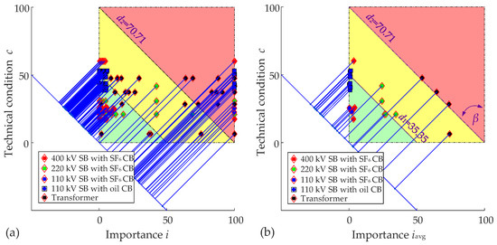
Figure 2.
(a) c − i diagram for all bays and transformers in all significant states; (b) c − iavg diagram for all bays and transformers with average value of importance.
The RCM diagram in Figure 2 represents a graphical representation of the main data, which are the importance and technical conditions of elements from Table 2. The importance of elements was averaged, due to the need for a better visualization and request for a uniform solution for the determination of maintenance frequency of elements.
The bay code in Table 2 consists of one letter and three digits. The letter represents the type of bay: line bay (L), transformer bay (T), or bus coupler bay (C).
The first digit indicates the voltage level of the bay (1–110 kV, 2–220 kV, and 4–400 kV). The last two digits represent the sequence number of the bay. The code for power transformers consists of two letters (Tr) and three digits. The first digit indicates the voltage level of the primary winding, the second is the secondary winding, and the third is the sequence number of the transformer.
Figure 2a shows the c − i diagram with the condition of all elements in all significant states of the index ijq, while Figure 2b shows the c − iavg diagram with the average index of the element iq. In comparison to the diagram in Figure 2a, the diagram in Figure 2b shows only one point on the c − i diagram for the TS elements. d1 and d2 are bounds between the areas of action and are defined by the TSO. These areas represent risk of failures on devices.
The colors in the c − i diagram describe the kind of maintenance tasks. In the green area, there are prescribed regular inspections of HV devices; in the yellow area, there are maintenance interventions that require equipment revision; and in the red area, there are the cases where the equipment needs to be replaced. The deviation dq defines as to which area an individual TS element belongs [1,26].
From the diagram (Figure 2b), it is evident that 110 kV bays were in the green-yellow border area (110 kV circuit breakers). The 220 kV bays were in the same area, only their importance was higher. The 400 kV bays were, due to their importance in the transmission system and recent replacement, in the green area. The transformers were in the yellow-red area, due mostly to their age and importance for the EPS. Their replacement was planned for the near future. Δp was negligible for all SF6 SB in TS. It was set to Δp = [Δpq = 0].
3.2. Costs
Table 3 contains the data on expected costs of outages and maintenance costs for the example presented in this paper. The nine columns for SSs present the costs Cin,jq of long duration outages for all significant states, defined in Section 2.7. The last two columns contain total costs Cin,q of outages for each element, calculated using (3), and revision costs Cr,q for each element defined in Section 2.6.
Table 3.
TS elements’ costs.
4. Optimization Process of Maintenance Activity
The concept of optimization is based upon seeking for the minimum maintenance costs in the observed period, which is usually one year with regard to the TSO, and taking into consideration the reliability of operation.
A block diagram of the optimization process and analysis of the optimal data is shown in Figure 3. The diagram is linked to the diagrams in Figure 1 through the connections A–F.
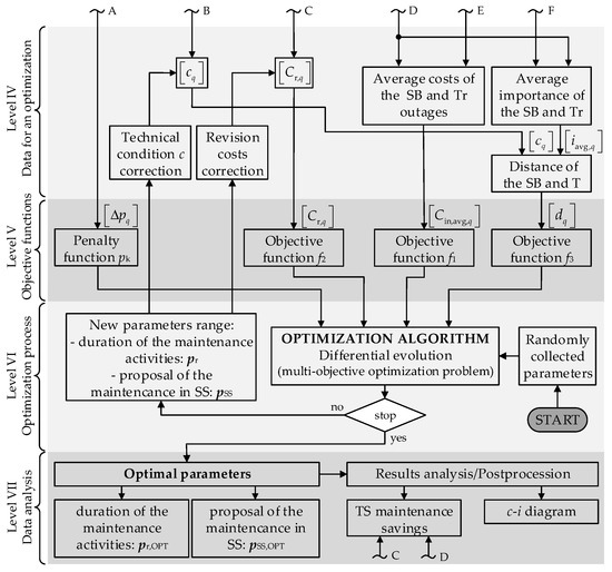
Figure 3.
Algorithm of the optimization process of maintenance.
4.1. Objective and Penalty Function
The maintenance model is linked to the optimization algorithm with objective and penalty functions. Three objective functions and one penalty function were defined to achieve the reliability-based maintenance concept. Since the objective functions are related to different quantities, they are normalized in the optimization process to enable merging of criteria.
The first objective function f1 is related to the expected costs of outage during the maintenance for all significant states. Figure 4a shows the fuzzy function (bell-shaped membership function) used to normalize the expected costs of non-transmitted energy Cin,q. The concept of normalizing is such that the costs of non-transmitted energy, which in “usual” significant states lie between xl = 5 and xu = 300 EUR/year, represent 90% variability of the normalized value. The costs of expected outages Cin,q that occur several times per year amount to approximately EUR 1,000,000 per year (Table 3) and have no more impact on the value of the objective function.
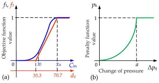
Figure 4.
(a) Presentation of normalization of the objective functions f1 (expected costs of outages) and f3 (c-i indices); (b) presentation of normalizing of the penalty function pk (leaking of SF6).
The second objective function f2 in the optimization process that represents the revision costs for a certain TS element Cr,q for all tasks that require de-energizing of an individual bay. Since the range of these costs is smaller than for the first objective function, there is no need for the use of fuzzy function-based normalization. The normalization is performed using (7)
The third objective function f3 is related to the indices of the RCM maintenance concept. In the block diagram of input data (Figure 3), the RCM indices c and i are included in the common index d. In the denotation of the vector, the weighting factor wSSj needs to be taken into consideration. For the determination of the objective function f3, the common part dq is used, which includes all the above-mentioned factors. An easier insight into the situation is enabled by the c − iavg diagram, shown in Figure 2b. If the value of dq is lower than 35.3 (green area), this objective function yields f3 = 0. If the value of dq lies between 35.3 and 70.7 (yellow area), the value of the objective function f3 is linear between 0 and 1. If the value exceeds 70.7 the value of the objective function is f3 = 1. The third objective function is illustrated graphically in Figure 4a.
Penalty function pk is related to the variations of pressure of the greenhouse SF6 gas in the circuit breakers. The penalty function describes that the leaking of SF6 in the period Δt is the reason for more frequent maintenance interventions. The higher the change of pressure in the period Δt, the steeper is the penalty function pk, i.e., the sooner it approaches the value of 1 (Figure 4b). If the pressure drops below the factory-set value a, the protection disables operation of the HV device, which requires a maintenance intervention—replacement of the element. The equation of the penalty function (8) can be derived from Figure 4b.
The optimization algorithm for maintenance of transmission substations, designed in the above-described way, is referred to as a multiobjective optimization algorithm. The most commonly used approach for solving the multiobjective optimization problem is the use of the weighted sum method f = γ1 ∙ f1 + γ2 ∙ f2 + γ3 ∙ f3 + pk, where the optimization algorithm finds an unambiguous solution with regard to the selected weights γ1, γ2, and γ3 of the objective function. Weights are chosen empirically: γ1 = 0.25, γ2 = 0.25, and γ3 = 0.5. The highest weight is assigned to the third objective function, due to the higher importance of the RCM concept. Equal weights are assigned to the first and the second objective functions that deal with maintenance and operation costs. The reason for this decision is in the final reduction of overall costs, since we believe that performing of maintenance activities based on the RCM concept contributes significantly to the reduction of associated risks and rational use of financial funds.
4.2. Optimization Parameters
In the optimization procedure, two optimization parameters are selected for each bay nSU. The first optimization parameter represents the periods of revision that are performed on every TS bay. Three periods were selected: every year, every two years, and every three years. The vector of revision pr, which is defined by pr = [pr,q]; pr,q ∈ {1,2,3}, can be created for all bays and transformers. The second parameter of the optimization procedure represents the SS-based maintenance (Table 1). This parameter defines for each TS bay and transformer the most suitable SS for performing of revision. The vector of maintenance by SS pSS is created for all TS bays and transformers. The codomain of this vector is the significant states themselves. The parameter is defined by pSS = [pSS,q]; pSS,q ∈{j; 1 ≤ j ≤ nSS}; 1 ≤ q ≤ nSU; j,q ∈ N.
4.3. Optimization Process with the Modified Differential Evolution Algorithm
The modified differential evolution algorithm, which belongs to the group of evolutionary computation methods, is used in the optimization process. In the process of seeking the optimal solution of the objective function, which represents the maintenance model of a substation on the basis of the RCM concept, we introduced a modification of the algorithm, representing self-adaptation (SA) of the control parameters CR in F [29,30]. The following three possibilities were analyzed: optimization without SA (basic DE algorithm), optimization with CR and F self-adapted for the entire population, and optimization with CR and F self-adapted for each individual in the population.
These improvements ensured adequate robustness of the algorithm since the optimization problem is extremely complex and comprehensive (62 optimization parameters).
To ensure successful operation of the DE optimization algorithm, we selected the control parameters of differential evolution that are presented in Table 4. The control parameters have a significant impact on performance of the search process in DE (convergence of the optimization process and accuracy of computation of the optimal solution).
Table 4.
Control parameters of DE.
5. Results of Optimal RCM Maintenance
The use of an adequate optimization tool can ensure preservation of the existing level of maintenance quality, despite the cost reduction achieved by the use of the modified differential evolution algorithm.
5.1. Optimization Process
The progress of optimization process versus iterations is shown in Figure 5. It can be seen that the optimization process converged to the optimal solution after approximately 700 iterations.
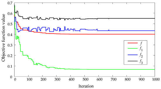
Figure 5.
Progress of the optimization process of common objective function and partial objective functions.
Seeking an optimal solution in the optimization process is conditioned by the values of individual objective functions and their weights. Individual objective functions, of course, cannot converge to their own optimums, since the optimization process is oriented to the common criterion that represents the correlation of individual criteria.
Ten independent calculations of optimization algorithm runs were performed for each SA variant. The average value and standard deviation of the objective function were computed on the basis of these runs (Table 5). The use of an optimization algorithm without SA indicates a dispersion of the results of 10 independent runs. The results of both other variants with the use of SA, on the other hand, indicate the reliability and robustness of the optimization algorithm, since there was no dispersion of the results of 10 independent optimization runs (standard deviation equals zero). All results are related to the optimization with SA.
Table 5.
Mean values and standard deviation of objective function for variants of SA.
5.2. Optimal Maintenance for the Observed TS
The optimization was performed to obtain optimal parameters representing the frequency of maintenance activities pr,OPT and the optimal SS pSS,OPT, in which the maintenance should be carried out. The maintenance of each TS bay is, therefore, conditioned by two optimization parameters.
Figure 6 shows the results of optimal maintenance for the observed TS, where Figure 6a shows the optimization parameters from the vector pr,OPT (in years) for the revision performed in each individual switching bay or power transformers (the existing TBM maintenance methodology—red line, proposed optimal methodology—blue histogram). Figure 6b shows the optimal data of the second set of optimization parameters pSS,OPT, which represents the proposal for maintenance. It provides the information about the selected SS of the EPS (possible future combination of generation, consumption, and power flows in the TS) when it would be most suitable to de-energize the TS elements and perform revision.
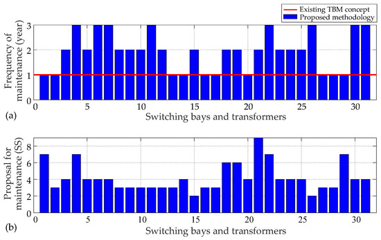
Figure 6.
Results of optimization. (a) Period of maintenance works (the existing TBM concept—red line, proposed optimal methodology—blue histogram); (b) proposal of maintenance in possible significant states.
The summaries of optimal parameters are in the form of histograms, shown in Figure 7. They show that it would be most suitable to perform revision on 10 elements every year, on 13 every two years, and on 8 every three years. With the proposed maintenance methodology, only approximately one-third of switchyard elements kept yearly frequency of maintenance activities. For the existing TBM concept, all 31 elements were found to have the frequency of maintenance activities every year. Despite the optimally selected maintenance periods, it would be necessary to perform revision on 10 elements every year. A comparison of the selected significant states in Table 1 and the histogram of the most suitable significant states led to the conclusion that the most suitable significant states for de-energizing state are the TS elements.
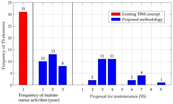
Figure 7.
Histogram of existing TBM concept and proposed optimal maintenance methodology.
The optimization results of RCM maintenance methodology are presented in the c − iavg diagrams in Figure 8. The c − iavg diagram after the optimization (Figure 8a) was compared with the c − iavg diagram before optimization (Figure 2b). The comparison of both c − iavg diagrams showed that the points only moved vertically. Differences between the values of technical condition index c before and after the optimization for individual switching bays ranged between 0 and 18.
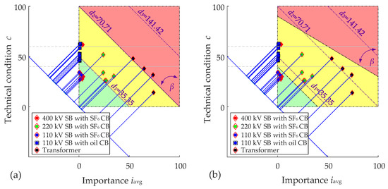
Figure 8.
(a) c − iavg diagram after optimization; (b) c − iavg diagram with changed maintenance areas.
In the optimization procedure, we also took into consideration the fact that the boundaries between maintenance areas of the bays on the c − iavg diagram could also be changed by varying the distances d1 and d2 or the angle β (Figure 8b). The determination of boundaries of individual areas in the c − iavg diagram depends on risks (outages of TS elements, financial risks) that the transmission system operator is willing to accept. Changing the boundaries and angle β in Figure 8b influences the maintenance concept. Any change of boundaries in the c − iavg diagram also influences boundary conditions of the optimization and requires a new run of the optimization tool.
The optimization process is performed with a feedback loop, which enables correction of new parameters of technical condition (index c) with regard to the period of the maintenance works, characteristic maintenance states, and performance of tasks. This ensures feedback to the input parameters through the index of technical condition c and a feedback loop to the optimization model.
The time window in the optimization model is three years, although the optimization is performed every year. This means that the time window is, every year, shifted by one year to the future. In the case of major investments to the TS the model is updated, and a new optimization run is performed. If there are no extraordinary events, the state of elements in principle does not change; otherwise, a correction is made that is considered in the optimization model for the time window of the next three years.
The purpose of introducing the optimization procedure in maintenance is not only to optimize costs by providing the highest reliability possible, but also in planning of maintenance tasks for the whole year.
5.3. Postprocessing of the Results
A comparison analysis of maintenance costs with the existing time-based maintenance and with the new RCM maintenance concept (Table 6) showed that the costs of the existing maintenance method amount to EUR 568,423, to which inspections contributed the main share. The optimization also influenced the revision activities in the three-year period.
Table 6.
Revision and total costs with and without optimization.
The savings were the highest in the first year, and amounted to 90.96% of the anticipated revision costs, or 25.53% of the total maintenance budget for the observed TS. In the second year, the savings were lower, and amounted to 66.83% of the anticipated revision costs, or 18.76% of the total maintenance budget for the observed TS. In the last year of the three-year period, the savings were the lowest, amounting to 24.13% of the anticipated revision costs, or 6.77% of the total maintenance budget for the observed TS.
The costs and savings shown above depend on the selection of weights γ1, γ2, and γ3 in the objective function. The selection of weights can provide more importance, either to the introduction of RCM maintenance or costs, i.e., reliability, or savings. The TSO needs to decide which aspect is more important. Table 6 shows the costs and savings for the selection of weights, described in Section 4.1 (γ1 = 0.25, γ2 = 0.25, and γ3 = 0.5), where higher importance is given to RCM maintenance, i.e., reliability. For comparison, Table 7 shows costs and savings for the following selection of weights: γ1 = 0.5, γ2 = 0.25, and γ3 = 0.25.
Table 7.
Revision and total costs with and without optimization for changed objective function weights in the optimization process.
The selection of weights in Table 7 brings in the first year a 95.50% saving of predicted revision costs and 26.78% of the total maintenance budget of the substation. In the second year, the savings were lower, amounting to 82.13% of the predicted revision costs and 23.06% of the total maintenance budget. In the third year, the savings were the lowest, amounting to 17.87% of the predicted revision costs and 5.02% of the total maintenance budget. The maximum difference between savings in the revision costs from Table 6 and Table 7 was 15.3%.
6. Discussion
In the field of maintenance of electric power system devices and networks, time-based maintenance (TBM) is still used widely. Nevertheless, a large number of companies are gradually introducing condition-based maintenance (CBM). An upgrade of such maintenance system is RCM, wherein the frequency of maintenance interventions is defined with regard to the state and importance of the EPS element. RCM maintenance methodology considers the reliability of the entire system and not only individual elements, which is the key advantage of this maintenance methodology.
An RCM model was developed and tested for transmission substations. For this purpose, in the first step, input data were defined for the indicators of operational reliability, technical condition of devices, and maintenance costs. These data were obtained on the basis of results of diagnostics and monitoring of elements, as well as from the calculations of parameters for the entire Slovenian EPS. The RCM model was upgraded with an optimization algorithm that enables it to find the optimal maintenance costs at the guaranteed reliability of operation and the most suitable combination of generation, consumption, and power flows (SS). Improper maintenance of the EPS elements causes various risks. These risks can be managed by the introduction of maintenance optimization. For the maintenance costs to be reduced, it is necessary to know the limit of acceptable risks. The maintenance optimization mode presented in this paper was tested practically in one of the Slovenian transmission substations. The developed algorithm is universal and can be used for any TS and included in the entire process of EPS maintenance, i.e., in the asset management of any transmission system operator.
A limitation of use of the proposed algorithm can, in the case of very large maintenance systems (e.g., a few thousands of elements), be problematic. In such a case, the use of conventional optimization algorithms, such as the one used in this paper, could jeopardize the stability of the optimization process and the accuracy of the obtained solutions.
With the proposed new algorithm for calculating maintenance periods using the optimization process, we confirmed the hypothesis that analyzing the past data of operation, events, and maintenance costs enables a direct impact on maintenance process for the future periods. With this maintenance concept, we maintain the reliability of operation of EPS elements and of their technical condition. At the same time, we reduce maintenance costs. A comparison of the existing (TBM) maintenance concept and the proposed one confirms savings. The proposed computations showed 25.53% saving in the first year, 18.76% in the second year, and 6.77% in the third year. This was the confirmation of the second hypothesis.
Further research work in the field of EPS elements’ maintenance enables extensions of the optimization model on all substations and all transmission lines in the transmission system. Testing with different maintenance periods could be performed for more extensive comparisons. It would also be possible to perform research of the use and testing of different optimization algorithms, as well as introduction of new approaches, such as the deep learning maintenance process.
Author Contributions
Conceptualization, P.K. and J.R.; methodology, P.K. and L.B.; software, P.K. and J.R.; validation, L.B., J.P., and J.R.; formal analysis, J.P.; investigation, L.B. and J.P.; resources, L.B. and J.P.; data curation, L.B.; writing—original draft preparation, P.K.; writing—review and editing, J.P. and J.R.; visualization, P.K.; supervision, J.P. and J.R.; project administration, J.P. All authors have read and agreed to the published version of the manuscript.
Funding
This research received no external funding.
Institutional Review Board Statement
Not applicable.
Informed Consent Statement
Not applicable.
Data Availability Statement
Not applicable.
Conflicts of Interest
The authors declare no conflict of interest.
References
- Balzer, G. Condition assessment and reliability centered maintenance of high voltage equipment. In Proceedings of the 2005 International Symposium on Electrical Insulating Materials (ISEIM 2005), Kitakyushu, Japan, 5–9 June 2005; pp. 259–264. [Google Scholar]
- Birkner, P. Field experience with a condition-based maintenance program of 20-kV XLPE distribution system using IRC-analysis. IEEE Trans. Power Deliv. 2004, 19, 3–8. [Google Scholar] [CrossRef]
- Bohatyrewicz, P.; Płowucha, J.; Subocz, J. Condition Assessment of Power Transformers Based on Health Index Value. Appl. Sci. 2019, 9, 4877. [Google Scholar] [CrossRef] [Green Version]
- Zhang, F.; Wen, Z.; Liu, D.; Jiao, J.; Wan, H.; Zeng, B. Calculation and Analysis of Wind Turbine Health Monitoring Indicators Based on the Relationships with SCADA Data. Appl. Sci. 2020, 10, 410. [Google Scholar] [CrossRef] [Green Version]
- Liu, Y.; Xv, J.; Yuan, H.; Lv, J.; Ma, Z. Health Assessment and Prediction of Overhead Line Based on Health Index. IEEE Trans. Ind. Electron. 2019, 66, 5546–5557. [Google Scholar] [CrossRef]
- Fang, F.; Zhao, Z.; Huang, C.; Zhang, X.; Wang, H.; Yang, Y. Application of Reliability-Centered Maintenance in Metro Door System. IEEE Access 2019, 7, 186167–186174. [Google Scholar] [CrossRef]
- Vera-García, F.; Pagán Rubio, J.A.; Hernández Grau, J.; Albaladejo Hernández, D. Improvements of a Failure Database for Marine Diesel Engines Using the RCM and Simulations. Energies 2020, 13, 104. [Google Scholar] [CrossRef] [Green Version]
- Zhang, X.; Zhang, J.; Gockenbach, E. Reliability Centered Asset Management for Medium-Voltage Deteriorating Electrical Equipment Based on Germany Failure Statistics. IEEE Trans. Power Syst. 2009, 24, 721–728. [Google Scholar] [CrossRef]
- Ge, H.; Asgarpoor, S. Reliability and Maintainability Improvement of Substations With Aging Infrastructure. IEEE Trans. Power Deliv. 2012, 27, 1868–1876. [Google Scholar] [CrossRef]
- de França Moraes, C.C.; Pinheiro, P.R.; Rolim, I.G.; da Silva Costa, J.L.; Junior, M.D.S.E.; Andrade, S.J.M.D. Using the Multi-Criteria Model for Optimization of Operational Routes of Thermal Power Plants. Energies 2021, 14, 3682. [Google Scholar] [CrossRef]
- IEC Standard 60300-3-11. In IEC Dependability Management-Part 3-11: Application Guide-Reliability Centred Maintenance; IEC: Geneva, Switzerland, 2009.
- IEC Standard TS 62775. In IEC Application Guidelines-Technical And Financial Processes for Implementing Asset Management Systems; IEC: Geneva, Switzerland, 2016.
- Mohd Selva, A.; Azis, N.; Yahaya, M.S.; Ab Kadir, M.Z.A.; Jasni, J.; Yang Ghazali, Y.Z.; Talib, M.A. Application of Markov Model to Estimate Individual Condition Parameters for Transformers. Energies 2018, 11, 2114. [Google Scholar] [CrossRef] [Green Version]
- Yang, F.; Chang, C.S. Multiobjective Evolutionary Optimization of Maintenance Schedules and Extents for Composite Power Systems. IEEE Trans. Power Syst. 2009, 24, 1694–1702. [Google Scholar] [CrossRef]
- Rafiei, M.; Khooban, M.-H.; Igder, M.A.; Boudjadar, J. A novel approach to overcome the limitations of reliability centered maintenance implementation on the smart grid distance protection system. IEEE Trans. Circuits Syst. II Express Briefs 2020, 67, 320–324. [Google Scholar] [CrossRef]
- Bahrami, S.; Rastegar, M.; Dehghanian, P. An FBWM-TOPSIS Approach to Identify Critical Feeders for Reliability Centered Maintenance in Power Distribution Systems. IEEE Syst. J. 2020, 15, 3893–3901. [Google Scholar] [CrossRef]
- Hilber, P.; Miranda, V.; Matos, M.A.; Bertling, L. Multiobjective Optimization Applied to Maintenance Policy for Electrical Networks. IEEE Trans. Power Syst. 2007, 22, 1675–1682. [Google Scholar] [CrossRef]
- Arno, R.; Dowling, N.; Schuerger, R. Equipment Failure Characteristics and RCM for Optimizing Maintenance Cost. IEEE Trans. Ind. Appl. 2016, 52, 1257–1264. [Google Scholar]
- Piasson, D.; Bíscaro, A.A.P.; Leao, F.B.; Mantovani, J.R.S. A new approach for reliability-centered maintenance programs in electric power distribution systems based on multiobjective genetic algorithm. Electr. Power Syst. Res. 2016, 137, 41–50. [Google Scholar] [CrossRef] [Green Version]
- Zhang, D.; Li, W.; Xiong, X. Overhead line preventive maintenance strategy based on condition monitoring and system reliability assessment. IEEE Trans. Power Syst. 2014, 29, 1839–1846. [Google Scholar] [CrossRef]
- Suwnansri, T. Asset management of power transformer: Optimization of operation and maintenance costs. In Proceedings of the 2014 International Electrical Engineering Congress (iEECON), Chonburi, Thailand, 19–21 March 2014; pp. 1–4. [Google Scholar]
- Dong, M.; Zheng, H.; Zhang, Y.; Shi, K.; Yao, S.; Kou, X.; Ding, G.; Guo, L. A Novel Maintenance Decision Making Model of Power Transformers Based on Reliability and Economy Assessment. IEEE Access 2019, 7, 28778–28790. [Google Scholar] [CrossRef]
- Hinow, M.; Mevissen, M. Substation Maintenance Strategy Adaptation for Life-Cycle Cost Reduction Using Genetic Algorithm. IEEE Trans. Power Deliv. 2011, 26, 197–204. [Google Scholar] [CrossRef]
- Pandzic, H.; Conejo, A.J.; Kuzle, I.; Caro, E. Yearly Maintenance Scheduling of Transmission Lines Within a Market Environment. IEEE Trans. Power Syst. 2012, 27, 407–415. [Google Scholar] [CrossRef]
- Zhong, J.; Li, W.; Wang, C.; Yu, J.; Xu, R. Determining Optimal Inspection Intervals in Maintenance Considering Equipment Aging Failures. IEEE Trans. Power Syst. 2017, 32, 1474–1482. [Google Scholar] [CrossRef]
- Belak, L.; Marusa, R.; Ferlic, R.; Pihler, J. Strategic Maintenance of 400-kV Switching Substations. IEEE Trans. Power Deliv. 2013, 28, 394–401. [Google Scholar] [CrossRef]
- McDonald, J.D. Electric Power Substations Engineering, 2nd ed.; CRC Press: Boca Raton, FL, USA, 2006. [Google Scholar]
- Wang, F.; Tuinema, B.W.; Gibescu, M.; Meijden, M.A.M.M. Reliability evaluation of substations subject to protection system failures. In Proceedings of the 2013 IEEE Grenoble Conference, Grenoble, France, 16–20 June 2013. [Google Scholar]
- Brest, J.; Greiner, S.; Boskovic, B.; Mernik, M.; Zumer, V. Self-adapting control parameters in differential evolution: A comparative study on numerical benchmark problems. IEEE Trans. Evol. Computat. 2006, 10, 646–657. [Google Scholar] [CrossRef]
- Glotić, A.; Glotić, A.; Kitak, P.; Pihler, J.; Tičar, I. Parallel Self-Adaptive Differential Evolution Algorithm for Solving Short-Term Hydro Scheduling Problem. IEEE Trans. Power Syst. 2014, 29, 2347–2358. [Google Scholar] [CrossRef]
Publisher’s Note: MDPI stays neutral with regard to jurisdictional claims in published maps and institutional affiliations. |
© 2021 by the authors. Licensee MDPI, Basel, Switzerland. This article is an open access article distributed under the terms and conditions of the Creative Commons Attribution (CC BY) license (https://creativecommons.org/licenses/by/4.0/).