Wall Structure Geometry Verification Using TLS Data and BIM Model

Abstract

Building information modeling (BIM) represents significant progress in the field of digitalization and informatization of the construction process. The virtual model (BIM model) is the source of graphic data among other information, which are applicable for geometry verification of the building’s structures. For this purpose, data and information about the building should be collected. Comparison of the BIM model (design) with as-built 3D models enables the evaluation of the quality of the as-built structures. The most effective methods for spatial data collection are terrestrial laser scanning (TLS) and close-range photogrammetry. Using both methods, measurement can result in a point cloud. The paper describes an approach for verifying the geometry of wall structures. The graphic data of designed structures are represented by the existing BIM model. The approach presented uses the Industry Foundation Classes (IFC) file format from which the designed geometry is derived. The as-built models of the structures are created from point clouds. Point cloud segmentation uses a combination of regression, filtering based on local normal vectors, and curve segmentation. Consequently, the designed and the as-built models (segmented from the point cloud) are compared.

1. Introduction

Building information modeling (BIM) enables digitalization of the whole life cycle of a building, from the design, through construction to operation. It is a process that uses a consistent and continuously updated model [1]. The use of BIM brings more simple and effective access to information, generates benefits for all partners (investor, designer, and constructor), and leads to possible reductions in the investment process [2,3,4,5]. Using a common data environment for information sharing improves the onsite collaboration and communication with such efficiency, which cannot be compared to drawing sets in a form of separate files. BIM enables model-based cost estimation in the planning stage of the construction, clash detection, and very effective coordination and collaboration with contractors. 5D planning enables not only construction scheduling, but also financial planning of the construction. Finally, well-coordinated and verified models lead to increasing the quality of the building. Several carried out analyses prove that most of the companies that have adopted BIM achieved an overall reduction of costs. Therefore, there is significant attention put into BIM worldwide, focusing on model creation and management of investment processes in the construction industry [6,7,8]. A BIM model is an object-oriented virtual model of the building, which consists of three parts in terms of data involved. The first part is graphic data defining the geometry and, in most cases, it is a 3D model. The second and third parts are non-graphic data, representing information and parameters, and documentation respectively. The detail of a BIM model is defined by the standard ISO 19650-1:2018 Organization and digitization of information about buildings and civil engineering works, including building information modelling (BIM)—Information management using building information modelling—Part 1: Concepts and principles.

Early identification of changes (deviation between the designed and built structures) in combination with high interoperability of partners using BIM enables to achieve savings during the construction project, thanks to good coordination of decisions about changes [2,9]. Therefore, the building industry needs timely and accurate information about these changes, which means measurement of the as-built geometry of the building. The verification often consists of a set of manual operations which require deep knowledge of the project, are time-consuming, and are costly. Graphic data of the BIM model are the source of information about the designed geometry of a building’s structure, and it is applicable for as-built verification of chosen parts or structural elements.

Currently, the most effective methods of spatial data collection are TLS and close-range photogrammetry resulting in point clouds. The use of information contained in detailed point clouds and information derived from a BIM model is a suitable tool for quality check of a given structure, often in real time. Combining the data from BIM with the data from TLS, the entire verification process, too, can be automated. TLS is available for a wide community of surveyors, structural engineers, and civil engineers thanks to the affordability and the fact that manufacturers of instruments make them easy to use with a high level of automation. This means, that during the scanning process, only some basic parameters (field of view and scan density) are needed to set up and the whole measurement is performed in an automated way. Therefore, TLS is used for different surveying jobs, e.g., [10,11,12,13,14,15,16,17,18,19]. Its main benefit is the efficiency of the 3D data collection (up to 2 million points per second), meaning less time spent on the construction site (needed for measurement) and often a huge amount of data defining the geometry of the surface of the measured structure [20]. The mentioned applies to TLS in general, the advantage or disadvantage of the chosen method depends on the specific scenario, instrument, and application.

The process of reconstruction of as-built BIM models from TLS data (scanned point clouds) is the so-called scan-to-BIM process [21,22,23]. As an analogy to this process, the comparison of the designed BIM model with the built structure from the TLS data is the scan-versus-BIM process. Several research efforts have been made in this area, which indicates the potential value of this process for progress monitoring and quality check of structural works. The scan-versus-BIM process is mostly divided into certain stages. To be able to compare the two models, in most cases this process starts with a transformation of the TLS data and the BIM model into the same coordinate system. This task can be executed in multiple ways, based on several survey points, or overlaps of surfaces (e.g., planar, spherical surfaces, etc.) between the two models. In addition, various techniques have been proposed for automated or semi-automated registration [24]. The second part of this process is deviation estimation, this part can also be done in various ways. Most frequently, it is realized by computing the minimum distances between the TLS data and the nearest surface from the BIM model for every point of the point cloud. Another frequently used way is to compute the distances in user-specified directions (e.g., in the direction of the common coordinate system axis, or the direction of the plane’s normal vector, etc.). Further, in some applications, the point cloud is divided into segments based on the BIM model objects, i.e., each point of the point cloud is paired with the closest 3D object from the designed BIM with some tolerance (the segments are created as subsets in the close surroundings of the given structure). Then, each geometrical surface from the BIM model is compared with the paired sub-sets of points (identified and generated in the previous step). Chen et al. in [25] converted the BIM model into a mesh model, from which point clouds were generated for each face of the building structure. The TLS point clouds were then downsampled to have the same density as the point clouds generated from the BIM model. Deviations were calculated as point-to-point distances between the closest points of the two point clouds. Segments with the highest deviations were highlighted to mark the areas that require additional inspections.

The existing approaches compare the BIM model with the scanned cloud without detailed segmentation. The corresponding point cloud of the inspected element often contains objects that are not directly related to the surface of the element, which may affect the result when relative verification, e.g., when inspection of the flatness is performed. Another limitation is that they only check the difference in position of the chosen structural part and do not deal with the inspection of the geometric parameters. The contribution of the paper is a proposal of a new approach for verification of the position and also flatness of wall structures.

The last part of the scan-versus-BIM process is the visualization of the computed deviations. There are also multiple possibilities, how to perform this task. The two most commonly used methodologies are color maps and contour lines. Individual setting of parameters for color maps can help to increase the lucidity of the results. Color maps can be divided into signed and unsigned. Unsigned color maps mean that the deviation values are visualized by their absolute value, so the points with the same absolute value will have the same color. On the other hand, in the case of signed color maps, the color for each value is visualized equivalently for positive and negative values. It is also possible to configure the range and the scale of the color map. Furthermore, for further processing and a better understanding of the results, a statistical analysis technique can be used to analyze the deviation patterns. For this issue, a deviation histogram for the individual segments can be generated to find the magnitude of the deviations between the two models. The histogram’s advantage against the color map is that it is easier to locate the magnitude of the deviations from the histogram [26,27,28,29].

The scan-versus-BIM process can be also performed with point clouds, which are generated from photogrammetric surveys. The advantage of cameras over laser scanners is, that they are more flexible to use, and they are financially more available. However, the final cost of using photogrammetry depends on the number of required images and the processing time. A disadvantage of using photogrammetry for data acquisition is that it is not as robust as TLS and the point cloud is the result of image processing (not raw result of measurement), which in some cases may lead to a lower geometric accuracy compared to TLS point clouds [30,31].

The paper describes an approach for verifying the geometry of wall structures using TLS data and BIM models. The advantages of the proposed approach over existing approaches are that it combines all the information that can be derived from a point cloud (3D geometry, RGB color, intensity of the reflected laser beam). An extended approach of evolving closed plane curve had been developed, which uses a fast and stable Lagrangean approach. The as-built models of structures are segmented from the measured point clouds. The designed and the as-built models are compared consequently. In addition, the flatness of the chosen structures is inspected and visualized.

2. Building Structures’ Geometry Verification

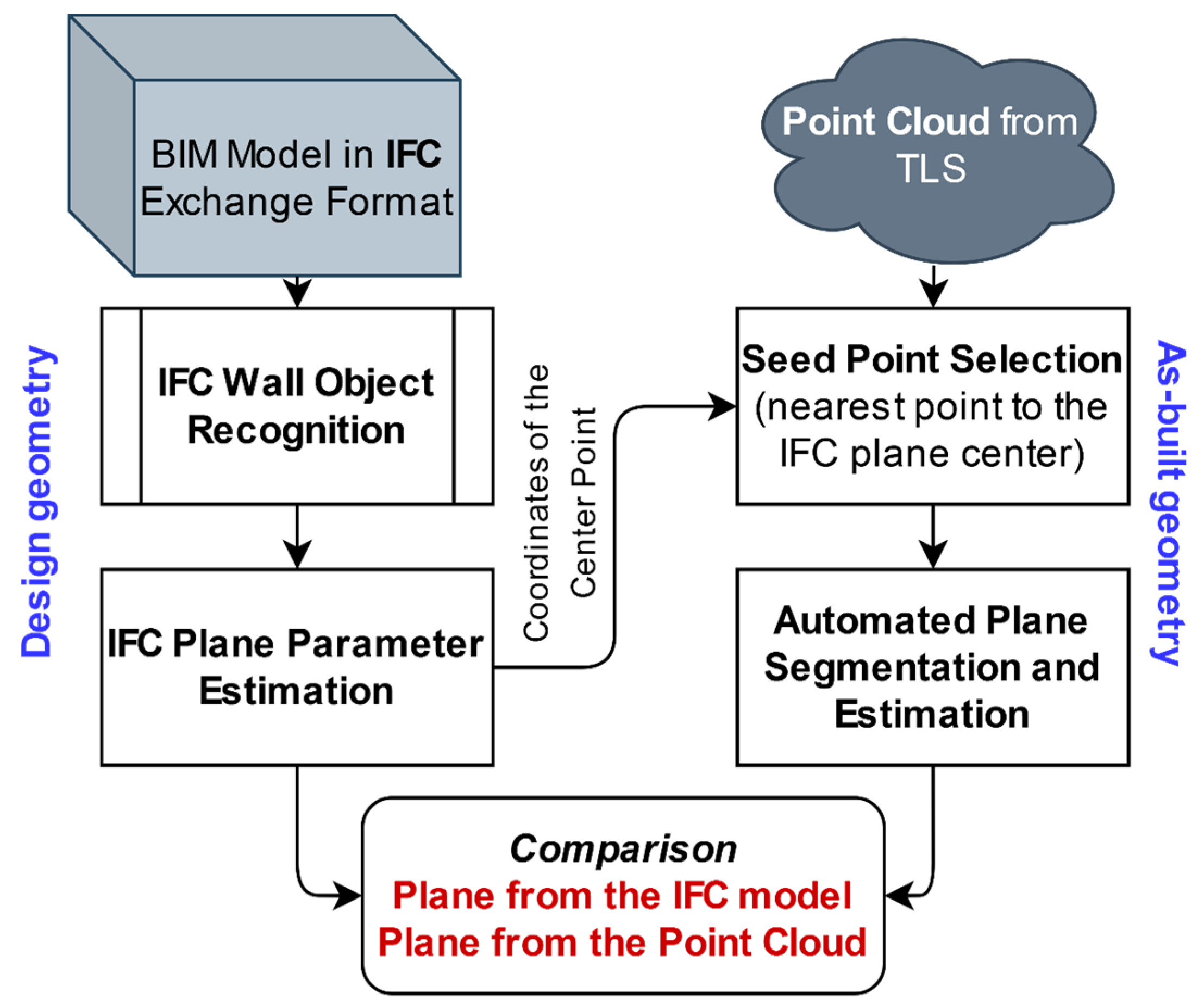
Verification of buildings’ structure means inspection (comparison to the design) the position, orientation (including verticality), dimensions, in case of planar surfaces (e.g., of walls) the flatness of a given structural element, and the relationship to other structures in terms of geometry. In the following, we describe the developed approach to enable verification of wall structures using point clouds and BIM models.

To ensure the highest possible level of automation, information about the planned geometry of buildings’ structural elements must be presented in digital form. This requirement is fulfilled using a BIM model, where data is stored in the graphic data of the information model. One of the key requirements of the entire BIM process is interoperability. The solution in this field is the use of a common data environment for sharing all the data related to the BIM process. In terms of geometry generation, it is also very important to use a “readable” data exchange format, which simplifies the procedure. Several file formats ensure appropriate storage of the model’s data, such as CAD formats, CIS/2, CityGML, etc. All of them are focusing on data for specific use. One of the most widespread data exchange formats worldwide is Industry Foundation Classes (IFC). IFC is an ASCII text file format that aims to provide open and neutral access to the storage and exchange of BIM models between different software. The format is developed by a non-profit organization buildingSMART, and it is defined by the standard ISO 16739-1:2018 Industry Foundation Classes (IFC) for data sharing in the construction and facility management industries—Part 1: Data schema.

The proposed and presented approach uses the data exchange format IFC and as-build data in form of a point cloud. The procedure can be divided into four main steps: identification and derivation of the geometry of building structures from the BIM model, segmentation of the point cloud (segmentation of the planes of walls’ surfaces), quantification of deviations, and creation of deviation maps (Figure 1). Each step is described in more detail in the following sections.

2.1. Geometry Identification from BIM Model

As mentioned above, the geometry of the verified structure is derived from the IFC file, which is a standardized (ISO 16739-1:2018) digital description of the building. It is a gradually evolving exchange format, and its current version is IFC4. Since IFC is formatted as a text file, it can be read using a text editor, which simplifies the procedure of the information derivation. For this purpose, it is necessary to know the structure of the data arrangement in IFC.

The IFC file consists of two main parts: the header and the data in the model. Within the data part are defined both the coordinate system and the system of units, which had been used. The coordinate system is a planar orthogonal, right-handed Cartesian coordinate system, which means that the coordinates X and Y are defined in the IFC but the Z coordinate, necessary for the definition of 3D space, is expressed by the height of the structural element. The form of coordinate definition does not correspond to the ones used in surveying, because it does not take into consideration map projection (Earth’s surface curvature, cartographic distortion) [32]. There is an IFC entity dealing with the map coordinate system called IfcMapConversion. However, its use only allows placement of the object at one point (easting, northing, orthogonal height) and orientation of the object towards the initial direction (north). For practical use, when modeling a larger area, it is necessary to divide it into parts (in local horizons) or apply coordinate corrections.

After defining the coordinate system and the units, the heights of individual floors of the building are defined and listed. The number of lines in this section depends on the total number of floors. The floors are defined by the IfcCartesianPoint and the IfcAxis2Placement3D entities. The first one defines the X, Y coordinates of the origin, which are in case of floors equal to 0, and the height of the floor. The IfcAxis2Placement3D entity defines the position in the coordinate system of the BIM model.

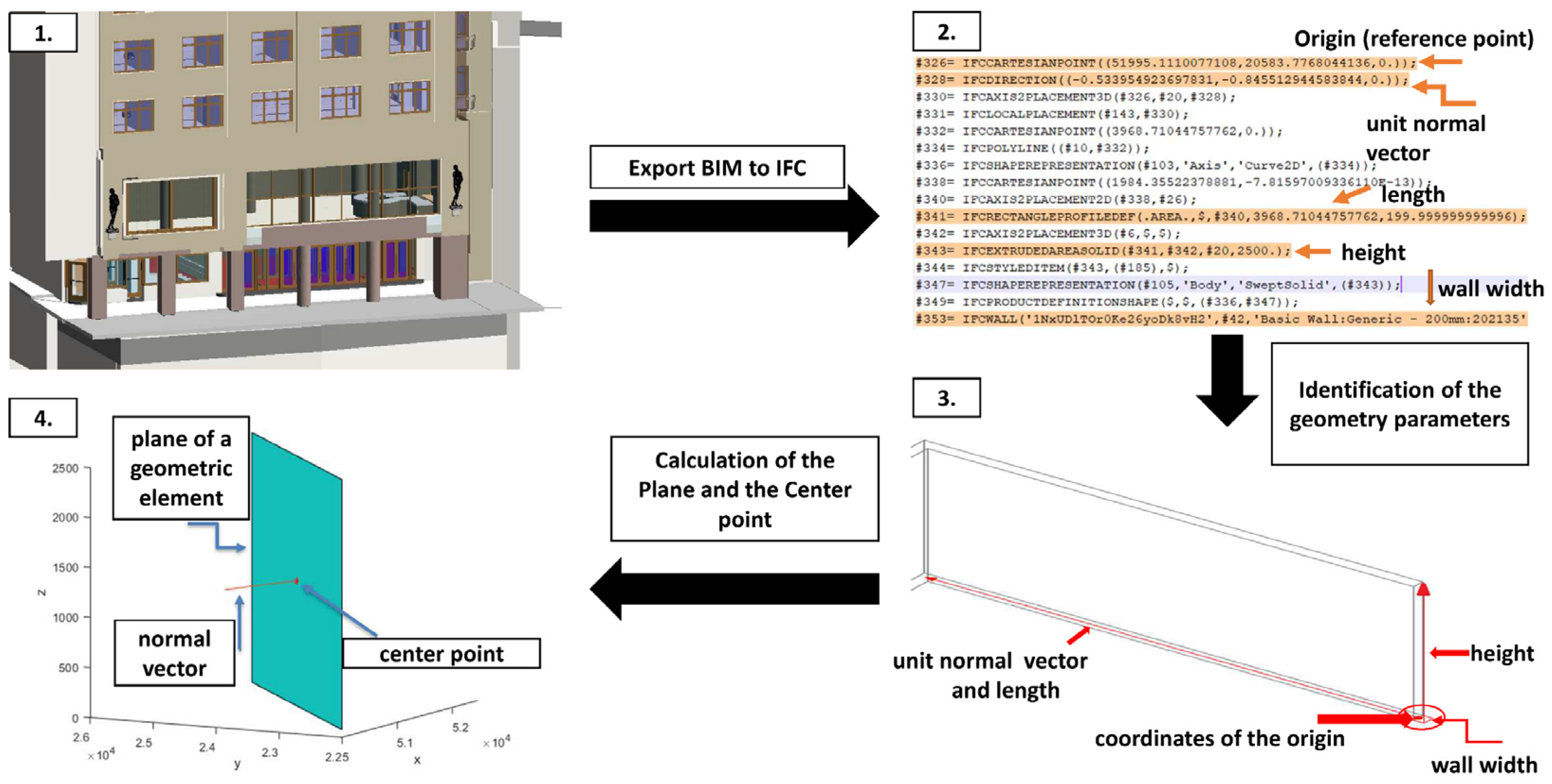
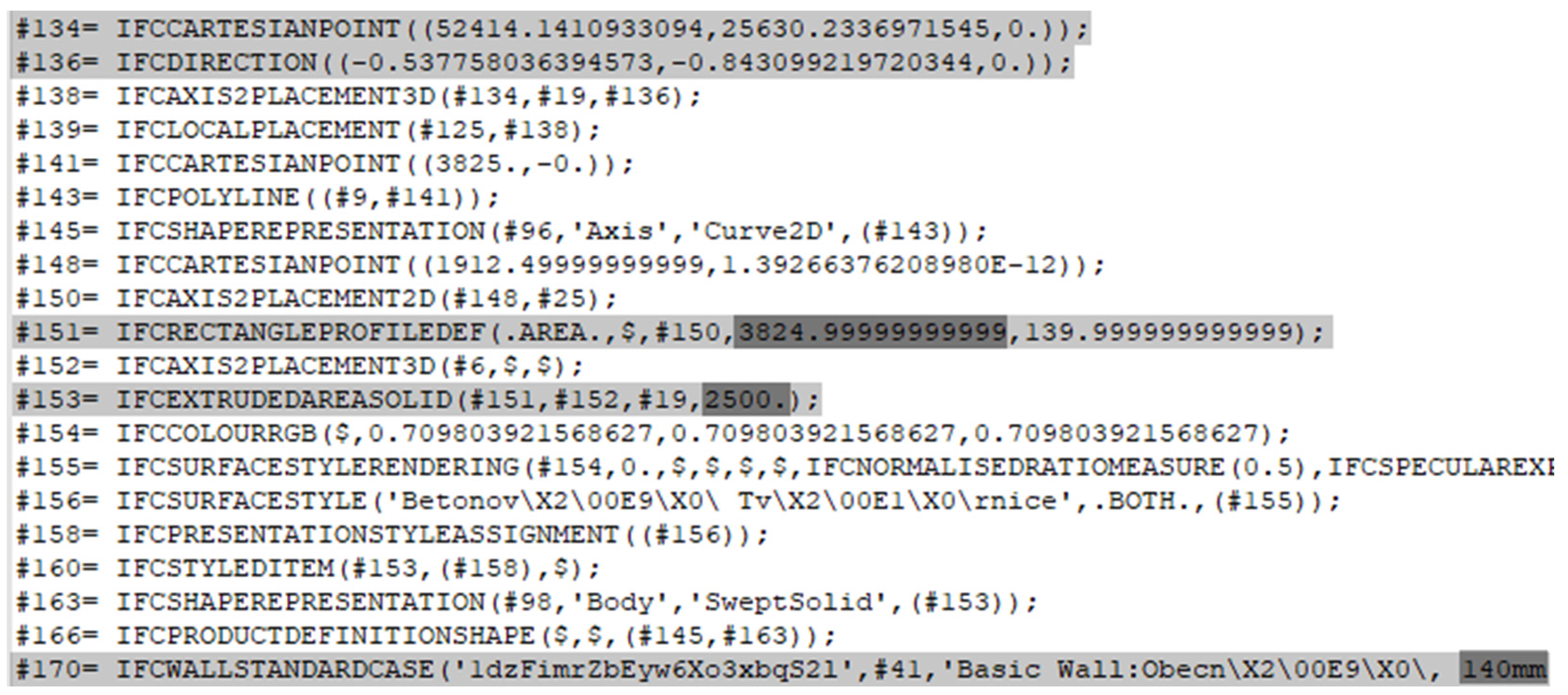
After this follows the definition of the building structures included in the given BIM model (Figure 2). Depending on the content of the model (e.g., foundations, walls, doors, windows, beams, columns, etc.), several sections are defining the structural parts, while the individual elements are defined in separate sections. It is not possible to directly estimate the length of the section, but the beginning and the end of each one can be identified. The section always starts with a coordinate of the origin of the geometric element, i.e., an IfcCartesianPoint line, and ends with the element name such as IfcWall, IfcDoor, IfcBeam, etc. Specific objects of interest of our approach are the walls, which in the IFC format are referred to as IfcWall. In the corresponding line, there is a specific wall number, which is a unique identifier. Subsequently, within the row, there is the thickness of the wall and the connection to the previous row, therefore, it is possible to identify where the wall is located and in which direction it is oriented. For each wall to be verified, it is necessary to obtain the coordinates of the reference point (origin), the direction vector of the wall, length, width, and height from the IFC file.

The coordinates of the reference point are obtained from the IfcCartesianPoint line (Figure 2). The direction is extracted from the line IfcDirection, which contains components of the unit direction vector. This line is missing in the case when the wall is oriented into the direction of the X or Y axis of the model’s coordinate system. This can be solved by comparison of the origin of two walls, where the direction can be derived from the changing X or Y coordinate of the origins. The height of the wall is in the IfcExtrudeAreaSolid line, while the length is defined by IfcRectangleProfileDef. In the case of a wall, we need an additional parameter which is thickness, defined in the IfcWall line.

From the five wall parameters directly derived from the IFC (coordinates of the reference point, direction, height, thickness, and length) the mathematical definition of the walls must be determined for verification of their geometry. Therefore, coordinates of the center point (center of gravity), and the coefficients of the general equation of the plane (wall surface) are estimated. The coefficients of the general equation include the components of the normal vector. Both planes of a wall are calculated, as both can be used in the further procedure. It depends on whether both planes were scanned and have to be verified or not. To calculate the center of gravity of a plane, first, we need to calculate the four boundary points (corners). The calculation is based on the well-known orthogonal surveying method using the coordinates of the reference point (origin) of the wall, from which we subtract or add the half of the wall’s thickness h recalculated to the direction of the coordinate system axis using the Equation (1):

$${\mathrm{X}}_1={\mathrm{X}}_{\mathrm{ref}}\pm \frac{\mathrm{h}}{2}\cdot {\mathrm{Y}}_{\mathrm{dir}},{\mathrm{Y}}_1={\mathrm{Y}}_{\mathrm{ref}}\pm \frac{\mathrm{h}}{2}\cdot {\mathrm{X}}_{\mathrm{dir}}$$

(1)

where X_ref, Y_ref are the coordinates of the reference point, h is thickness of the wall, and X_dir, Y_dir are the elements of the unit vector defining the direction of the wall. The plus or minus sign in the above equations is chosen according to whether we determine the inner or outer planes of the wall.

The remaining three boundary points (2, 3, 4) can be calculated similarly using Equation (1).

The center of gravity of the plane is calculated as the arithmetic mean of the four corners of the plane using the Equation (2):

$${\mathrm{X}}_{\mathrm{mean}}=\sqrt{\frac{1}{\mathrm{n}}}{\displaystyle \sum }_{\mathrm{i}=1}^{\mathrm{n}}{\mathrm{X}}_{\mathrm{i}},{\mathrm{Y}}_{\mathrm{mean}}=\sqrt{\frac{1}{\mathrm{n}}}{\displaystyle \sum }_{\mathrm{i}=1}^{\mathrm{n}}{\mathrm{Y}}_{\mathrm{i}},{\mathrm{Z}}_{\mathrm{mean}}=\sqrt{\frac{1}{\mathrm{n}}}{\displaystyle \sum }_{\mathrm{i}=1}^{\mathrm{n}}{\mathrm{Z}}_{\mathrm{i}}$$

(2)

where X, Y, and Z are the coordinates of the corners. Subsequently, two auxiliary vectors are calculated from three points of the plane according to (3):

$$u=\left[{\mathrm{X}}_4-{\mathrm{X}}_1,{\mathrm{Y}}_4-{\mathrm{Y}}_1,{\mathrm{Z}}_4-{\mathrm{Z}}_1\right],v=\left[{\mathrm{X}}_2-{\mathrm{X}}_1,{\mathrm{Y}}_2-{\mathrm{Y}}_1,{\mathrm{Z}}_2-{\mathrm{Z}}_1\right].$$

(3)

As the vector product of the vectors u and v, the normal vector n of the plane is calculated using Equation (4). Then, the general equation of the plane (5) can be defined from the calculated elements of the normal vector.

$$n=\left(\mathrm{a},\mathrm{b},\mathrm{c}\right)=\frac{u\times v}{\left|u\times v\right|}.$$

(4)

$$\mathrm{a}·\mathrm{X}+\mathrm{b}·\mathrm{Y}+\mathrm{c}·\mathrm{Z}+\mathrm{d}=0,$$

(5)

where d calculated by (6) is the scalar product of the normal vector of the plane and the position vector of the center of gravity.

$$\mathrm{d}=-\left(\mathrm{a}·{\mathrm{X}}_{\mathrm{mean}}+\mathrm{b}·{\mathrm{Y}}_{\mathrm{mean}}+\mathrm{c}·{\mathrm{Z}}_{\mathrm{mean}}\right).$$

(6)

The results of the algorithm for identification of the geometry of structural elements from IFC are the coordinates of the center points (centers of gravity) of individually verified walls, the unit normal vectors of walls’ planes, and the general equations of planes (Figure 3). After the wall plane segments are extracted from the as-planned IFC model, the corresponding planes are segmented from the as-built point cloud data. The procedure of this segmentation is described in the following section.

2.2. Plane Segmentation from Point Clouds

Segmentation is often the first step in gaining information from a point cloud. It means a division of a point cloud into several subsets of points based on predefined criteria. In most cases, the subsets contain points lying on the surface of the same geometric primitive (cylinder, sphere, plane, torus), lying on an irregular smooth surface, or forming edges of objects. The segmentation process, in this case, is the identification of geometric shapes in point clouds, and also the determination of their size, position, and orientation [33]. Based on the used algorithm, methods and approaches for point cloud segmentation can be divided into five groups [34,35,36,37]:

• Edge-based methods,
• Model-based methods,
• Surface-based methods, region-based methods,
• Clustering-based methods,
• Graph-based methods.

The algorithm for plane segmentation from point clouds, used in the presented approach, is partially inspired by the region-based segmentation method, while plane parameters are estimated by the least square method. The first step of the algorithm is the selection of a distance threshold. Points that are closer to the estimated plane than the selected threshold, are considered as inliers, and so points that are lying on the surface of the estimated plane. The segmentation process starts by selecting a small number of the nearest points (k-NN, e.g., 10 points, depending on the point cloud density) to a selected seed point. The seed point is the nearest point of the point cloud to the center point (center of gravity) of the extracted plane from the IFC model. Followingly, the parameters of a plane created by these points are estimated using orthogonal regression, which minimizes perpendicular distances to the estimated plane. The solution is based on the general equation of a plane [38].

The singular value decomposition (SVD) of the matrix of the reduced coordinates is used to calculate the components of the normal vector using (7):

$$A=U\Sigma V^{\mathrm{T}},$$

(7)

where A^n×3 is the matrix of reduced coordinates (reduced to the subsets centroid), n is the number of the selected number of neighboring points, the column vectors of U^n×n are normalized eigenvectors of the matrix AA^T, the column vectors of V^3×3 are normalized eigenvectors of the matrix A^TA. The matrix Σ^n×3 is a diagonal matrix with the first three singular numbers of the matrix A^TA on the main diagonal. Therefore, the normal vector of the regression plane is the column vector of V, which belongs to the smallest singular number of the matrix A^TA [38]. The components of the normal vector are the coefficients a, b, and c of the general equation of the estimated plane. The coefficient d is calculated by fitting the coordinates of the centroid point (X_mean, Y_mean, Z_mean), and the components of the normal vector to the Equation (8):

$$\mathrm{d}=-\left(\mathrm{a}·{\mathrm{X}}_{\mathrm{mean}}+\mathrm{b}·{\mathrm{Y}}_{\mathrm{mean}}+\mathrm{c}·{\mathrm{Z}}_{\mathrm{mean}}\right).$$

(8)

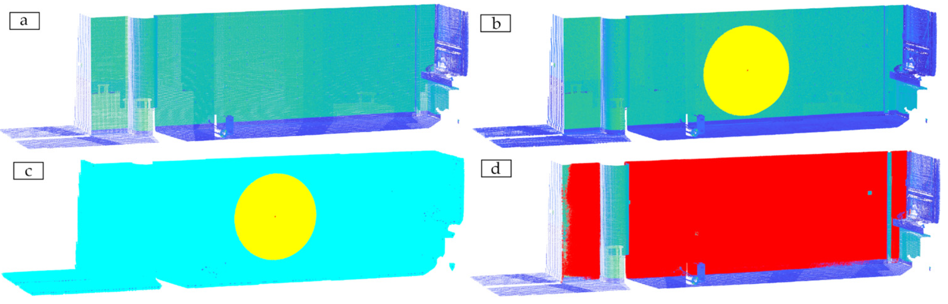
Then, the estimated plane model is tested against the selected neighbors, while points lying in this plane (volume defined by the plane and the distance threshold) are identified. This process is performed iteratively, with a gradual increase in the number of points tested. The gradual selection of the closest points for testing is illustrated in Figure 4. It shows the input point cloud (a), next to the 102,400 nearest neighbors (all the points inside the yellow circle) to the selected seed point (b), followed by the 1,638,400 nearest neighbors (colored by yellow and cyan) (c), and the inlier points (d) with red color for the chosen plane with the selected threshold value.

In every iteration, the inlier points are updated (from the nearest neighbors) based on distance criterion, and parameters of the plane are re-estimated using all the inlier points. The calculation (plane re-estimation) is repeated until the number of inliers stops increasing, so there are no more inliers for the selected plane.

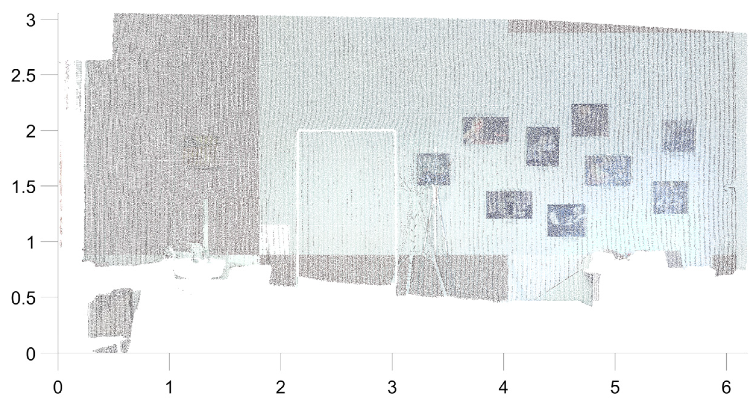
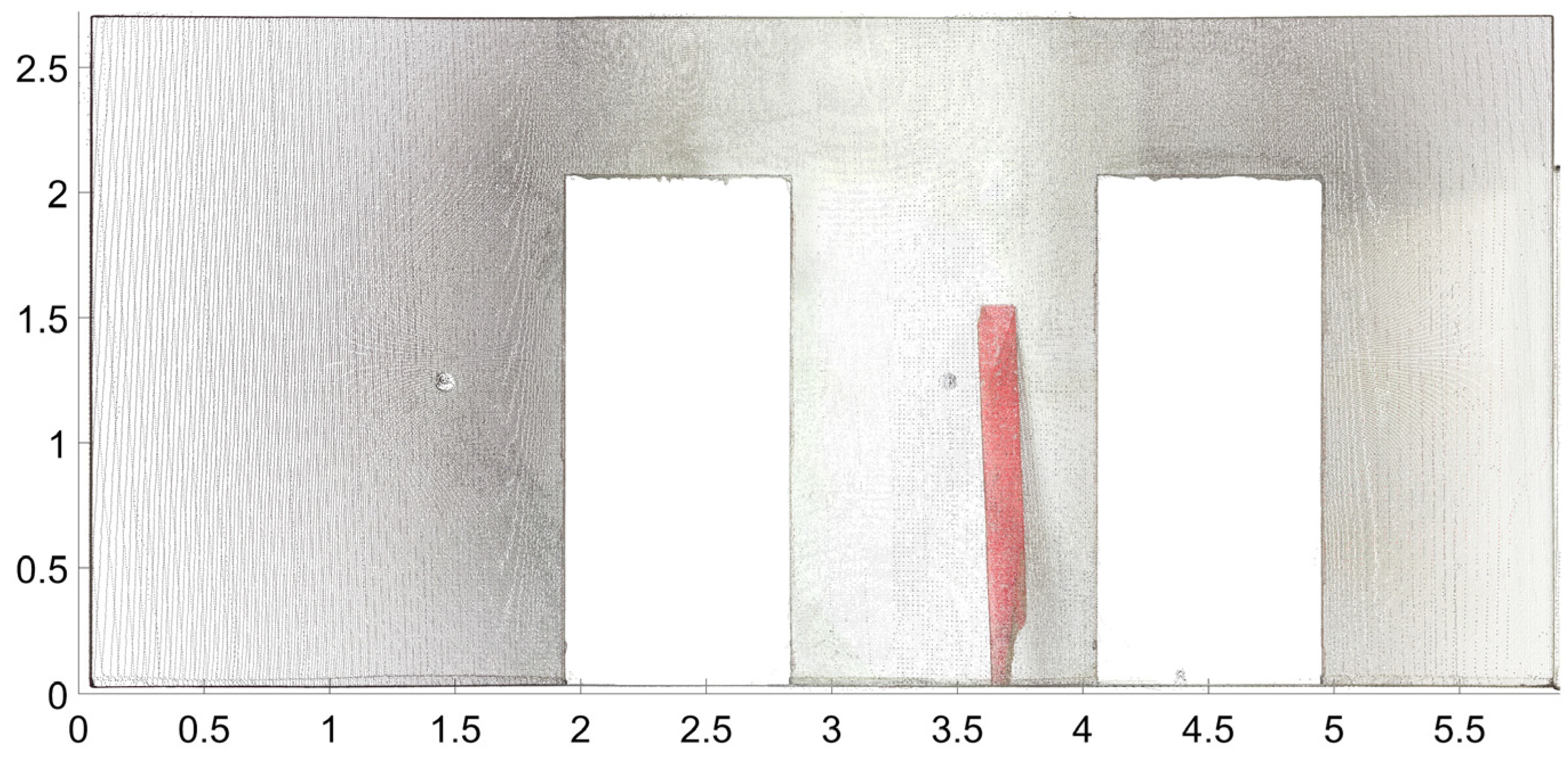
The steps described above automatically segment the point cloud to subsets containing points lying on the surface of the verified walls. Depending on the selected threshold value, also points in the close surroundings are segmented to the given subset. As Figure 5 shows, often there is a lot of other objects close to the scanned surface, especially when the building is in operation, but also on the construction site of a building under construction. The individual steps of our approach are demonstrated in an example of a studio in a theatre.

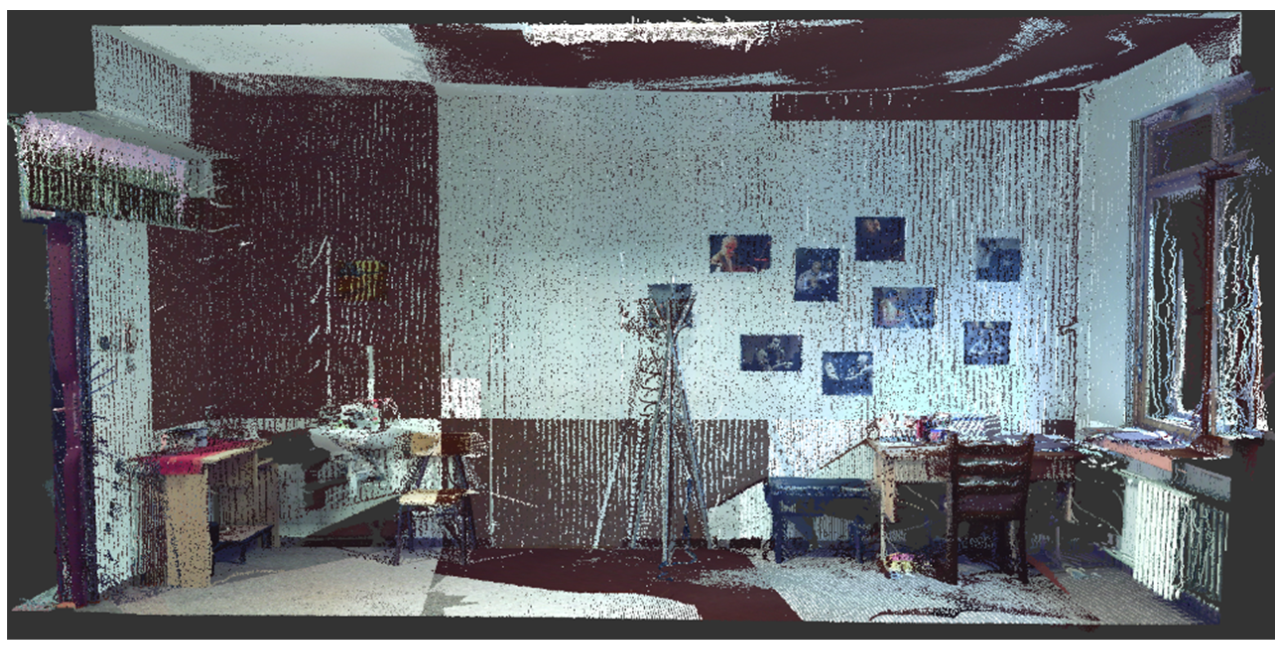
During the first step of the segmentation process, most of the furniture was removed, as these points do not meet the criterion defined by the distance threshold. The parts of the wall structure behind the removed objects (from the point of view of the laser scanner) are the empty areas in Figure 6. The points are colored, based on images taken by the instrument (RGB). The figure shows that the resulting subset of the point cloud also contains points not lying on the surface of the wall, e.g., posters, electrical sockets, and switches. The subset also contains doors. To solve the issue and to isolate points belonging to the surface of the walls, additional filtration procedures were created. These are based on local normal vectors and radiometric information (intensity, RGB) derived from the point cloud. The filtration can be divided into two main steps:

• Normal vector-based filtration,
• Curve segmentation.

Figure 6. Segmented point cloud—only distance-based filtering.

Figure 6. Segmented point cloud—only distance-based filtering.

2.2.1. Normal Vector-Based Filtration

The plane segmentation procedure, depicted in the previous section, uses distance-based filtering for inlier identification as the distance threshold is needed for the definition of the close surroundings of the wall. In practice, points of the objects close to the wall are also considered as inliers, if only the distance-based filtering is executed. However, these points are not lying on the surface of the verified wall (plane) as is shown in Figure 6.

After the initial plane segmentation, normal vectors at each point of the resulting subset of the point cloud are estimated using small local planes (calculated from the k-nearest neighbors). The selected number of k-nearest points depends on the point cloud density and noise. The value of k is set globally according to the average density of the point cloud. The calculated normal vectors are multiplied by the normal vector of the respective planes obtained after segmentation (9), and then the angle between them is quantified.

$$\cos \left(\mathsf{\alpha }\right)={∆}_{\mathrm{norm}}={\mathrm{n}}_{\mathrm{PoC}}·{\mathrm{n}}_{\mathrm{point}},$$

(9)

where n_point is the normal vector of the local plane calculated from k-nearest neighbors, n_PoC is the normal vector of the corresponding regression plane of the point cloud and α is the angle that the two vectors make at each other.

In order to perform the normal vector-based filtration, an angle threshold has to be defined. This threshold defines the maximum deviation of the local normal from the normal vector of the previously estimated regression plane. The recommended value of maximum deviation, based on our experience, is a small value between 2° and 4°. The choice of the threshold depends on the inspected wall. The proposed values mean deviations along 1 m of the structure 35 mm for 2° (in an extreme case it can be caused by nonflatness of the wall) and 70 mm for 4° (means that the subset of the point does not belong to a flat wall). This step removes the points from the segmented cloud that belong to the boundaries and curved parts of structural elements not directly related to the wall plane, e.g., the planes of the floor, ceiling, door frame, etc. (Figure 7).

However, after normal vector-based filtration, some points are still included in the inliers, while these are not belonging to the wall plane, e.g., points on doors, electrical sockets, paintings on the wall, etc. Therefore, a novel filtration approach based on evolving curves was proposed.

2.2.2. Curve Segmentation

The basic idea is to place a small segmentation curve (usually a circle) into the segmented region and expand the curve until it surrounds all points which belong to the surface of the wall. The evolution of the segmentation curves is driven by the properties of the points in the point cloud, e.g., color, intensity (of reflected laser beams), or distance from the regression plane.

The curve segmentation process consists of three main steps:

• Preprocessing: Creation of the input images from the planar point cloud.
• Evolution: Curve segmentation of the plane using images.
• Postprocessing: Creation of point cloud segments and selection of wall segment.

Preprocessing

To reduce the dimension of the problem, the almost planar point cloud is transformed (rotated and moved) to the new coordinate system in which the first two dimensions span the fitting plane. If we have a point with coordinates x = (x₁,x₂,x₃), the coordinates x₁ and x₂ describe the position of the point in the plane and the x₃ axis is orthogonal to the regression plane. 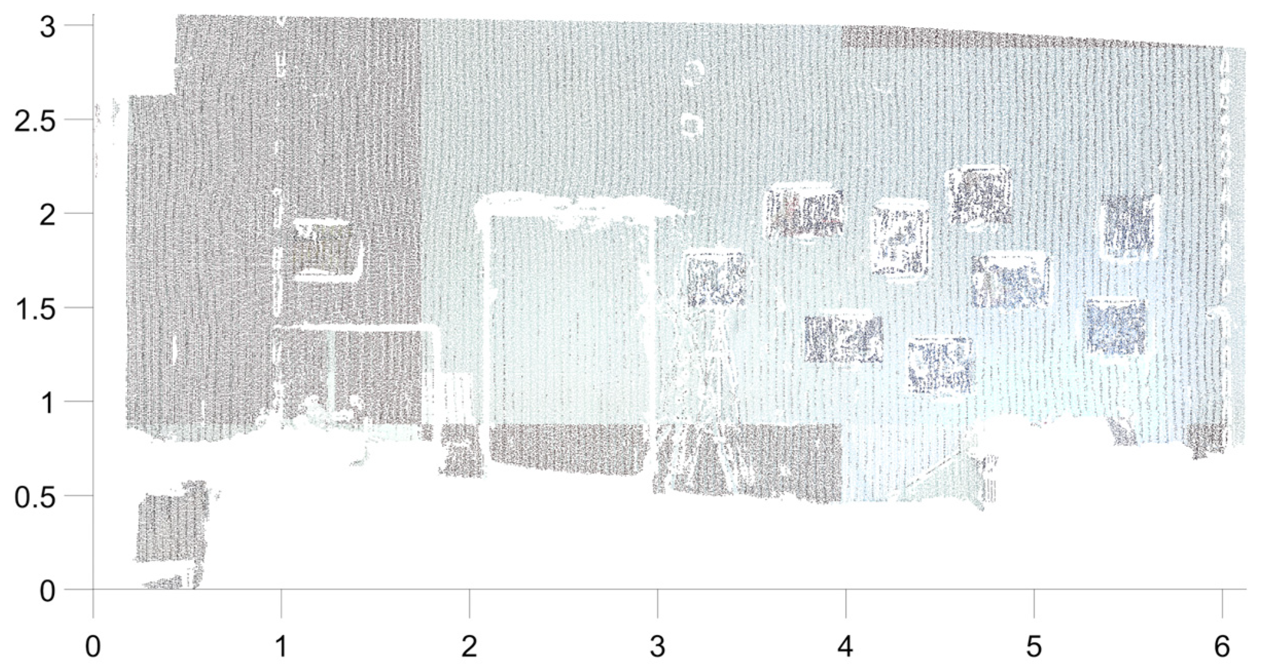First, we create a regular square mesh in the x₁, x₂ plane. Then, we represent the properties of the point cloud by a set of pixels (bitmap) images, one image for each property. For example, we take the R (red) channel of color and define the value of each pixel (square of the mesh) as the mean value of the R channel of all points which lie in the pixel. Finally, we rescale the values in each image to the interval [0,1]. Figure 8 shows the image for the intensity channel.

Evolution

The mathematical model is a modification and extension of the model described in more detail in [39]. The segmentation curve is an evolving closed planar curve with a position vector of its points denoted by x = (x₁,x₂). The evolution is driven by a suitably designed velocity field v, therefore, the basic evolution model is:

$$\frac{\partial x}{\partial \mathrm{t}}=v,$$

(10)

where ∂x/∂t denotes the time derivative of the position vector, i.e., the velocity of the point x. The equation is coupled with an initial condition—the initial curve is a small circle (or multiple circles) placed inside the segmented region.

The velocity v is considered in the form:

$$v=\left(1-\mathsf{\lambda }\left(\mathrm{t}\right)\right)B\left(x\right)N\left(x\right)+\mathsf{\lambda }\left(\mathrm{t}\right)\left(-\nabla E\left(x\right)\right)+\mathsf{\delta }\left(\mathrm{t}\right)k\left(x\right)N\left(x\right),$$

(11)

where N(x) denotes the positively oriented normal vector at point x of the curve, k(x) is the signed curvature at x, and ∇ is the gradient operator. The role of the first term BN is to expand the segmentation curve in the normal direction from its initial shape through the segmented region towards its border, the “blowing” function B controls the speed of the expansion and is defined using the bitmap images. The idea behind computing the value of B(x) for a point x on the curve is to compare the properties at point x to the average of the properties inside the evolving curve. If the properties are similar, the value of B(x) is large (the point x should move fast), if they differ a lot, B(x) is small (i.e., x should move slowly).

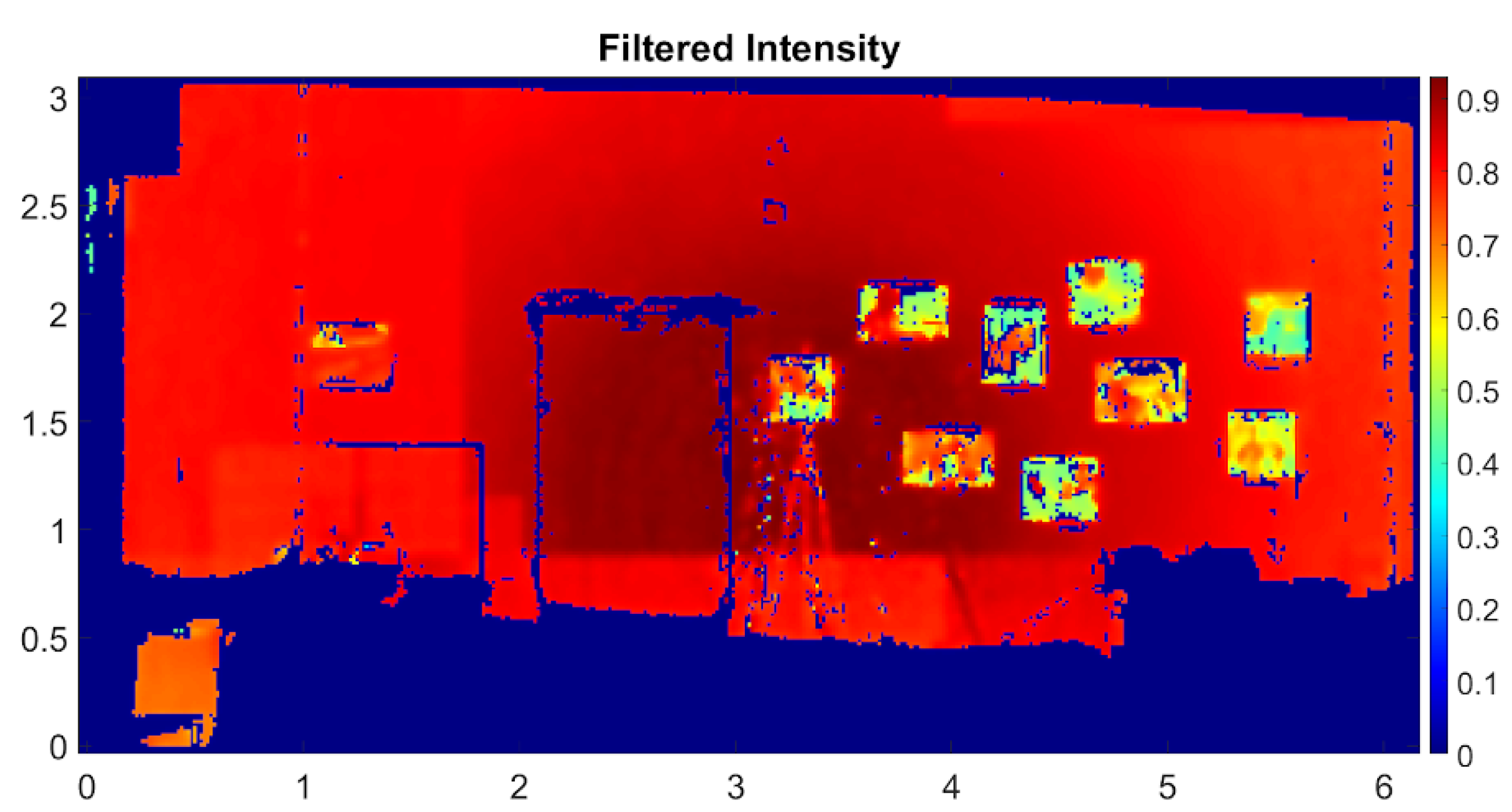
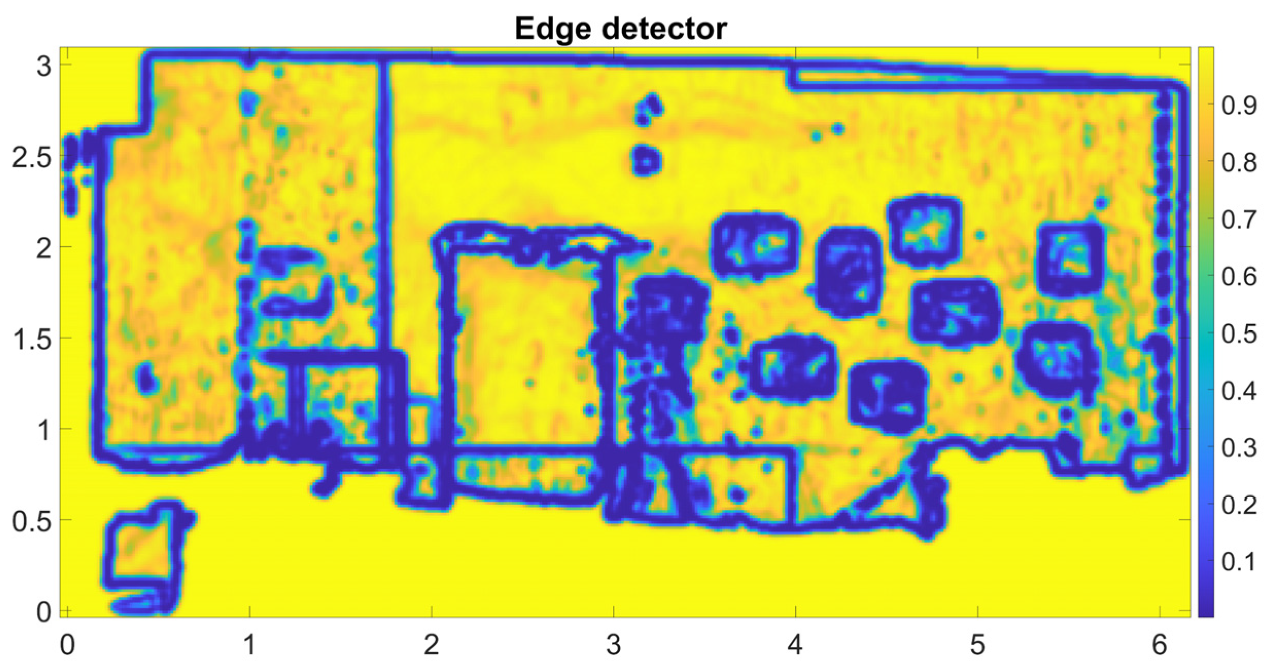
The second term attracts the points of the curve towards the borders of the segmented region. Information regarding borders is contained in the edge detector function E, which is computed using the gradients of the images (created in preprocessing step). The values of the edge detector E are close to 0 near edges and close to 1 in homogeneous regions (Figure 9). The negative gradient of E points towards the lower values (i.e., edges) and therefore is suitable to attract the segmentation curve towards the edges.

The time-dependent parameter λ(t) ∈ [0,1] serves as a weight between expansion and edge attraction term. The standard approach is to set λ(t) at the beginning of the evolution (t = 0) to a number 0 < λ₀ ≪ 1 (i.e., the edge attraction does not dominate), keep it unchanged until the curve is close to the border (moving very slowly) and then switch λ(t) to 1, which turns off the expansion and attracts the curve towards the edges.

The last term kN is called curvature regularization and has a smoothing effect. We use it to deal with the noise and to smooth sharp edges of the segmentation curve, mainly during the expansion phase. The parameter δ(t) weighs the influence of the term.

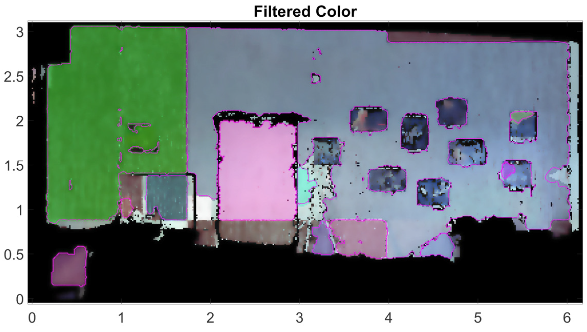
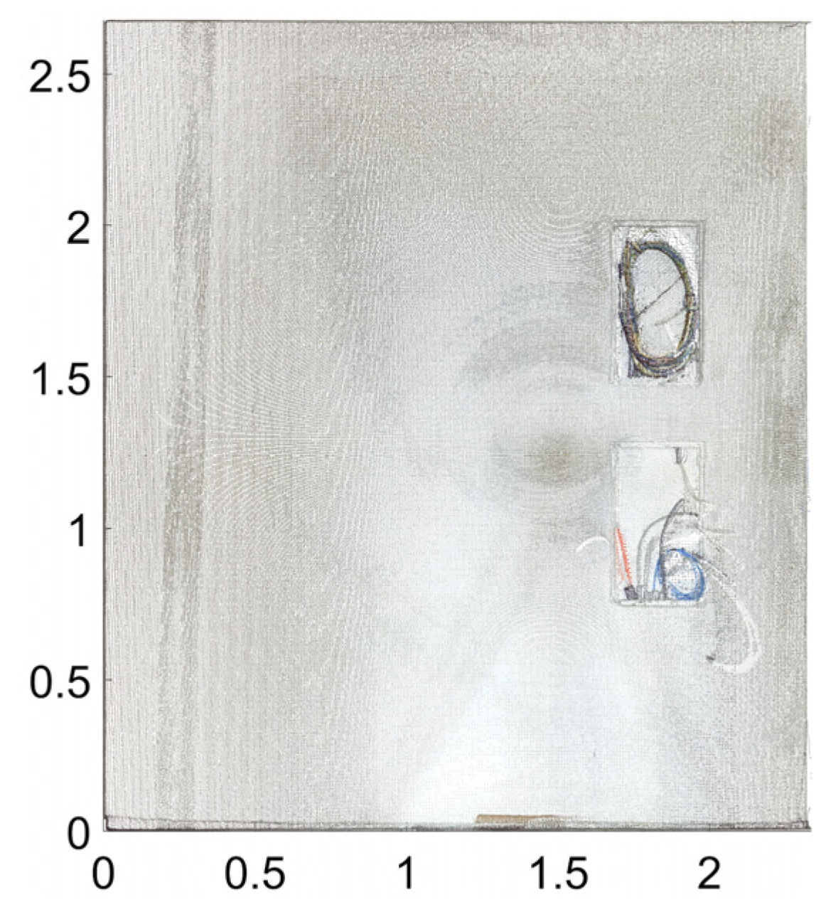
In practice, we can place many initial curves in the regression plane as well as create new initial curves during the segmentation. As the curves evolve, they can merge (if they have similar average properties inside) and split, too. Figure 10 shows the final segmentation curves.

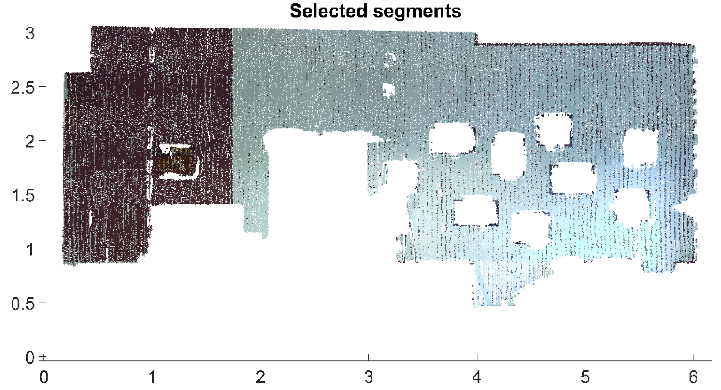
Postprocessing

After the evolution process is stopped, the subsets (segments) of the point cloud are created. For each final curve, the corresponding segment of the point cloud by selecting all points that lie in pixels inside the curve is created (in Figure 10 these pixels are colored by a specific color). As the last step, the segments that correspond to the segmented wall are chosen to obtain the result—the subset of the point cloud containing the points lying on the surface of the verified wall (Figure 11).

The parameters of the regression plane for wall flatness inspection are estimated from the subset of points after the above-described segmentation procedure. Orthogonal distances are calculated for each point of the segmented subset of points using (12). From the distances, a standard deviation is calculated which reflects the precision of the plane surface determination.

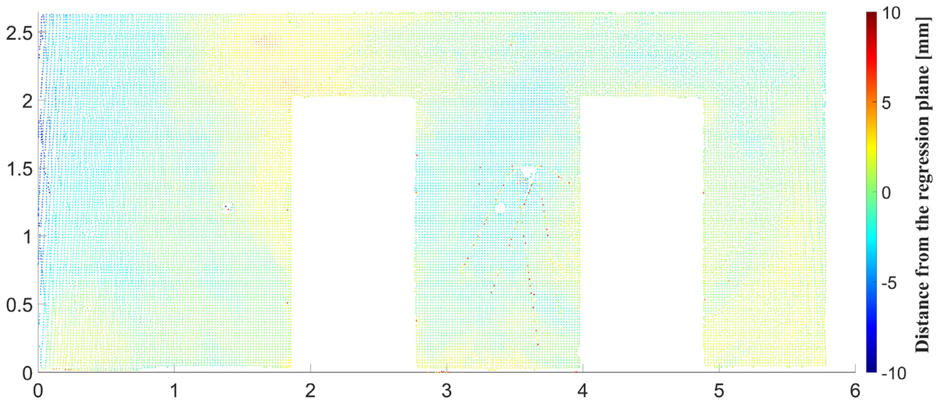
2.3. Creation of Deviation Maps

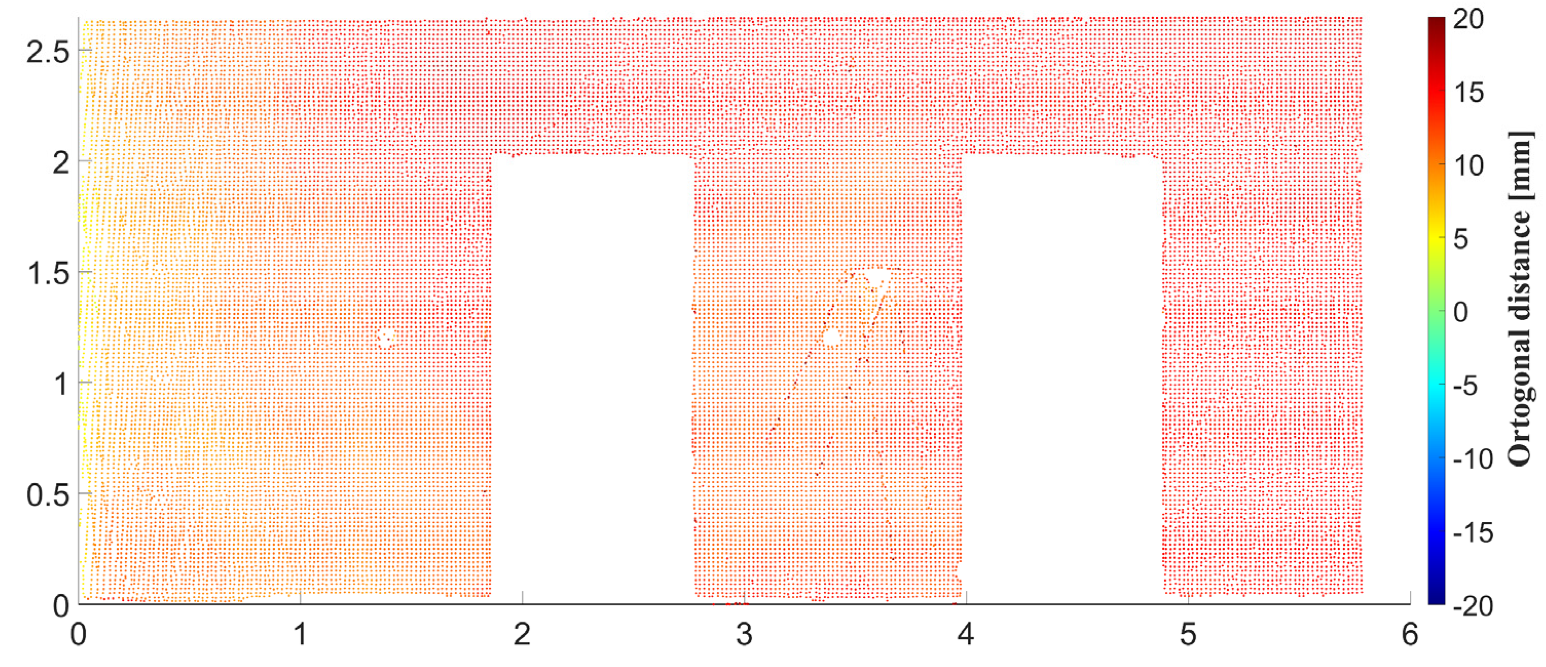
The last step of the approach for building structures’ geometry verification according to the flowchart in Figure 1 is the comparison of the as-planned data derived from the BIM model and the as-built data from the point cloud. The deviations are expressed in the form of tables and deviation maps. Two deviation maps are generated for each wall plane. The first deviation map is created by comparison of the plane determined from IFC and the corresponding segmented subset of the point cloud (Figure 12). The distance of each point from the as-planned plane is calculated in the direction of the plane’s normal vector. The distances are calculated as a dot product of vectors containing the coordinate differences between the given point and the centroid point and the normal vector of the plane. The distances are positive if the point is on the same side of the plane as the normal vector and negative if it is on the opposite side. Considering the general equation of the plane (5) and the fact that the normal vector of the plane is normalized (with length equal to 1), the distances are calculated using Equation (12):

$$\mathrm{a}·{\mathrm{X}}_{\mathrm{P}}+\mathrm{b}·{\mathrm{Y}}_{\mathrm{P}}+\mathrm{c}·{\mathrm{Z}}_{\mathrm{P}}+\mathrm{d}=\mathrm{dist}.$$

(12)

where X_P, Y_P, and Z_P are the coordinates of a given point of the subset.

Subsequently, the points are colored according to the signed distances of the points from the plane. For practical use, especially in case of dense point clouds, the deviation map can be downsampled (e.g., 20 mm × 20 mm) to present the deviation map in the form of more homogeneously distributed points. It can be performed using grid average method, which means that the points within the same grid box are merged to a single point.

In addition to the deviation map, the rotation (difference between the orientation of normal vectors) and the deviation between both planes’ coefficient d are calculated. The rotation of the planes is calculated according to Equation (13):

$$\mathsf{\alpha }=\mathrm{acos}\left({\mathrm{n}}_{\mathrm{IFC}}·{\mathrm{n}}_{\mathrm{PoC}}\right),$$

(13)

where n_IFC is the normal vector of the wall plane from the BIM model and n_PoC is the normal vector of the estimated regression plane from the segmented point cloud. The deviation between the two models’ coefficient d is calculated using Equation (14):

$$\mathsf{\delta }=\left(\left|{\mathrm{d}}_{\mathrm{IFC}}\right|-\left|{\mathrm{d}}_{\mathrm{PoC}}\right|\right),$$

(14)

where d_IFC is the distance of the IFC plane from the origin of the coordinate system and d_PoC is the distance of the estimated regression plane from the origin of the coordinate system.

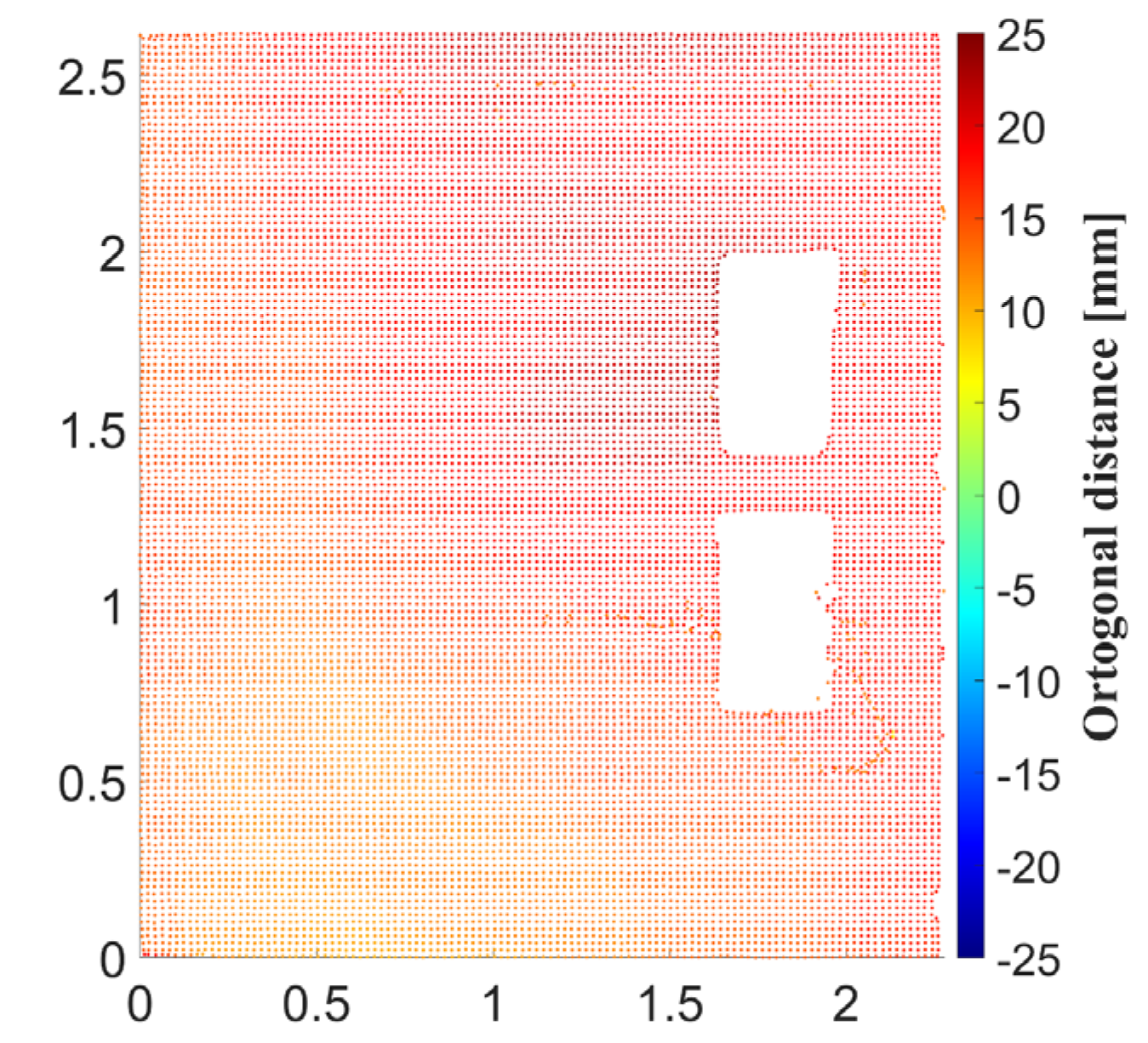
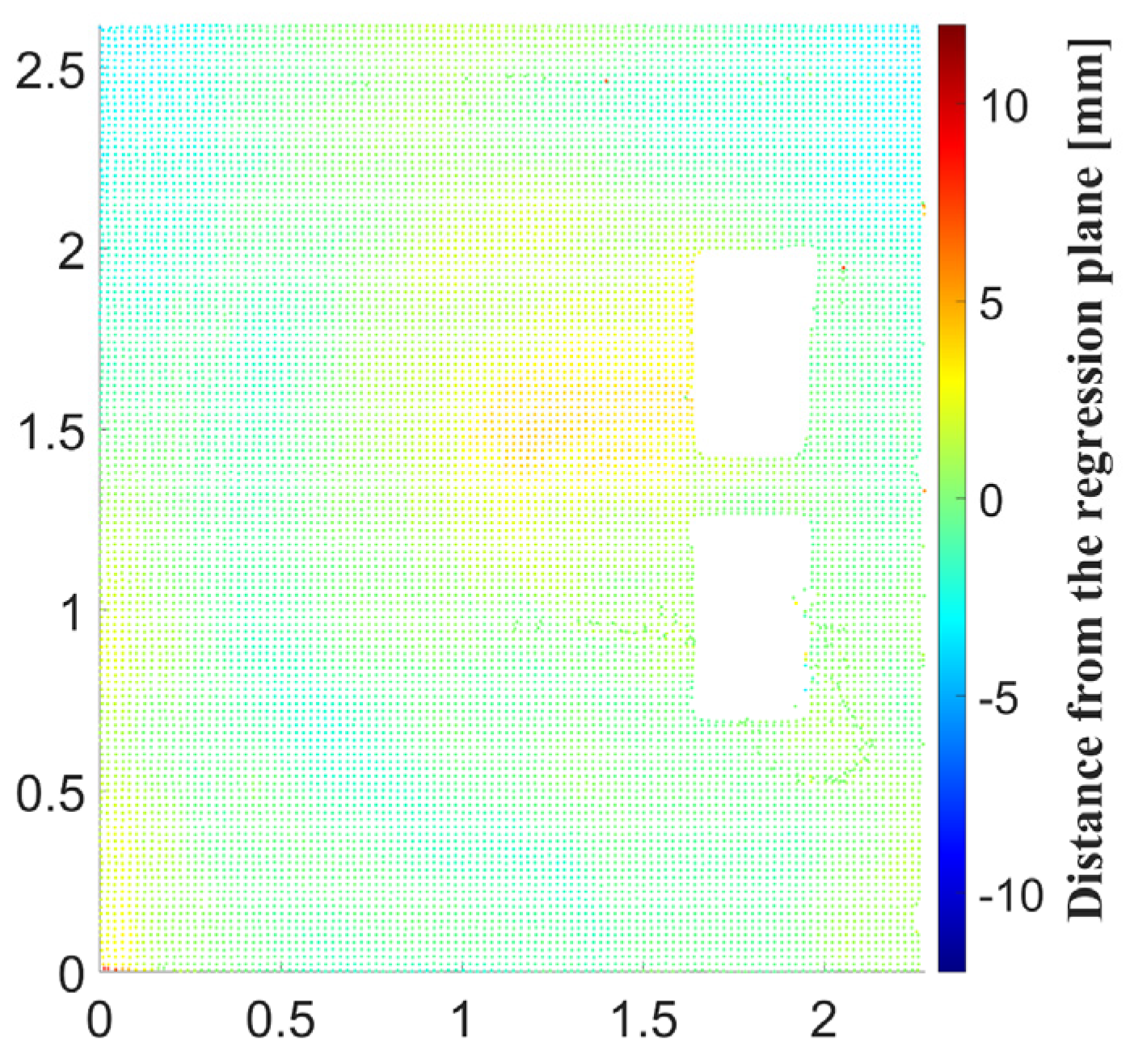
The second deviation map (generated for the same wall) quantifies the flatness of the wall (Figure 13). The flatness of the wall is calculated as the orthogonal distance of each point of the point cloud from the estimated regression plane using (12).

The advantage of the approach described above over existing methods is that a detailed segmentation and filtration of the point cloud is performed. Deleting points not directly related to the surface of the inspected wall increases the accuracy of the results. The biggest contribution of the paper in this field is the developed extended evolving plane curve segmentation, which identifies the openings and the objects not creating the surface of the wall. This is crucial in case of the flatness inspection of the walls, otherwise, the deviation maps will contain false information.

3. Case Study

In the case study, a three-room apartment was used (Figure 14). The apartment is part of a residential complex NUPPU in Bratislava with 800 apartments created by eight separate buildings. The BIM model of the apartment was provided by the contractor. The LOD of the model is 300, which means that the elements are graphically represented in the model as a separate system or object defined by quantity, size, shape, location, and orientation. The interior of the apartment was scanned using a terrestrial laser scanner Trimble TX5 with a scanning resolution of 1/16, which means 24.5 mm × 24.5 mm/10 m. The ranging error of the instrument defined by the producer is ±2 mm at 10 m. The whole interior was scanned from eight positions of the instrument. The scanned data were registered to the coordinate system of the design using surface-based registration (using overlapping areas) and target-based registration (using identical reference points) with a registration error of 3 mm. The described approach was performed on selected walls of the case study object. The numbering of the walls is shown in Figure 14.

The procedure described in Section 2 was used for this case study. The first step was the creation of wall segments from the derived corners from the IFC file. Segmentation of the corresponding subsets of point cloud was performed consequently. The threshold was set as 40 mm for distances and 4° for angles between normal vectors (for normal vector-based filtration).

Figure 15 and Figure 16 show the original point cloud (result of scanning) of selected walls colored in RGB. The walls are plastered with gray gypsum plaster. The color of the scanned surface in combination with the ambient light generates bright colors of points.

Results of the comparison of planes from the BIM model and planes estimated from the segmented subsets of points are listed in

Table 1. Comparison of the plane parameters.

n	aIFC	aPoC	bIFC	bPoC	cIFC	cPoC	dIFC [m]	dPoC [m]
1	1.0000	0.9999	0.0000	0.0023	0.0000	0.0006	−13.400	−13.444
2	−1.0000	−0.9999	0.0000	0.0022	0.0000	0.0005	16.235	16.252
3	1.0000	0.9999	0.0000	0.0013	0.0000	0.0004	−16.350	−16.378
4	−1.0000	−0.9999	0.0000	0.0005	0.0000	0.0014	19.250	19.240
5	0.0000	0.0021	−1.0000	−0.9999	0.0000	0.0010	−11.575	−11.552
6	0.0000	0.0030	−1.0000	−0.9999	0.0000	0.0019	−11.575	−11.524
7	0.0000	0.0006	1.0000	0.9999	0.0000	−0.0013	11.460	11.444
8	0.0000	−0.0022	−1.0000	−0.9999	0.0000	−0.0028	−9.760	−9.730
9	0.0000	−0.0013	−1.0000	−0.9999	0.0000	−0.0016	−10.060	−10.042
10	−1.0000	−0.9999	0.0000	0.0011	0.0000	0.0015	16.800	16.801
11	0.0000	0.0088	1.0000	0.9999	0.0000	0.0002	7.375	7.209
12	−1.0000	−0.9999	0.0000	0.0012	0.0000	0.0006	19.250	19.248
13	1.0000	0.9999	0.0000	0.0023	0.0000	0.0003	−15.700	−15.699

Where n is the number of the inspected wall, a_IFC, b_IFC, c_IFC, and d_IFC are the parameters of the plane from IFC, a_PoC, b_IPoC, c_PoC, and d_PoC are the parameters of the plane from IFC.

and

Table 2. Deviations between the BIM model and the as-built model.

n	$\mathsf{\alpha }$ [°]	$\mathsf{\delta }$ [mm]	max [mm]	min [mm]	avg [mm]	absmax [mm]
1	0.1346	−44	24	6	16	24
2	0.1279	−17	18	−9	11	18
3	0.0793	−28	20	4	11	20
4	0.0865	9	21	5	10	21
5	0.1338	23	23	6	14	23
6	0.2045	51	22	7	14	22
7	0.0815	16	20	2	12	20
8	0.2042	30	23	9	16	23
9	0.1192	18	21	7	13	21
10	0.1045	−1	26	7	16	26
11	0.5026	166	22	−4	9	22
12	0.0761	2	19	−1	9	19
13	0.1316	1	41	−3	14	41

Where n is the number of the inspected wall, $\mathsf{\alpha }$ is the difference between the orientation of normal vectors of IFC and regression plane, $\mathsf{\delta }$ is the deviation between the wall’s coefficient d, max and min are maximum and minimum deviations between the IFC plane and the segmented point cloud, avg is the average deviation between the IFC plane and the segmented point cloud, abs_max is the absolute maximum deviation between the IFC plane and the segmented point cloud.

. Table 1 contains parameters (a, b, c, and d) of the planes from IFC as well as the planes segmented and estimated from the point cloud. Table 2 shows the deviations in orientation and the deviation between the coefficients d (representing the distance of the plane from the origin of the coordinate system) of the corresponding planes and contains the maximum, minimum, and average deviations between the IFC plane and the segmented point cloud.

The maximal difference in orientation α between the planes is 0.5026° in the case of plane 11. The difference in orientation of 0.5° for a wall length of 2.45 m means a deviation of 21 mm. The absolute maximal difference of 41 mm between the IFC plane and the point cloud is in the case of wall no. 13. The average differences reached values from 9 mm to 16 mm. The standard deviation of the results of 4 mm is calculated applying uncertainty propagation law from the registration error and the uncertainty of the 3D position of a single measured point. It means that the deviations under the value of 4 mm are not significant. The deviations between the BIM model and the scanned surfaces, listed in Table 2, are caused by the uncertainty of the measurement (4 mm) and the construction deviation. The construction deviation can be characterized as a sum of the assembly deviation and setting-out deviation of the structures during the construction. Furthermore, the deviations may be caused by the fact that although the LOD of the model is 300, the plasters with a thickness of 10 mm were not modeled.

Figure 17 and Figure 18 show the deviation maps between the BIM model and the segmented point cloud for selected walls. The colors from green to red represents positive values in the color bars.

In

Table 3. Quantification of flatness of the walls.

n	max [mm]	min [mm]	absmax [mm]	std [mm]
1	5	−9	9	2
2	4	−16	16	2
3	7	−9	9	1
4	10	−15	15	2
5	7	−6	7	2
6	7	−5	7	2
7	10	−9	10	2
8	11	−5	11	2
9	5	−6	6	1
10	11	−9	11	1
11	10	−4	10	1
12	14	−5	14	2
13	19	−24	24	2

Where n is the number of the inspected wall, max and min are maximum and minimum deviations between the regression plane and the segmented point cloud, avg is the average deviation between the regression plane and the segmented point cloud, abs_max is the absolute maximum deviation between the regression plane and the segmented point cloud, std is the standard deviation calculated from the orthogonal distances of the segmented points from the regression plane.

, the results of the wall flatness quantification are listed, where are shown maximal and minimal distances between the regression plane and the segmented points. The deviations reached values from a maximum of 19 to a minimum of −24 mm. The standard deviations (std), calculated from the orthogonal distances of the segmented points from the regression plane, reached a maximum of 2 mm. The measurement of the flatness is an integral part of the inspections carried out. By classical measurement methods, this is measured as a deviation from a straight edge (usually 2 m long) using a measuring wedge. The inspected parts are chosen randomly, therefore, the result does not give a complex picture of the entire wall surface. The advantage of laser scanning is that the flatness is inspected on the whole surface of the wall. The tolerance defined by the standard EN 13914-2 Design, preparation and application of external rendering and internal plastering Internal plastering for the inspected walls is 5 mm along 2 m of the inspected structure. The deviation maps show the parts where the criterion was exceeded. In the case of flatness inspection, the accuracy of the results is affected by the dispersion of the points around the regression plane reflecting the random error (noise) of the measurement by TLS (coordinate determination) mainly. It is expressed by the standard deviation calculated from the orthogonal distances and listed in Table 3. In practice, it means that the values under the value of standard deviation are not significant, which in our case study means 2 mm.

Figure 19 and Figure 20 express the flatness of wall no. 7 and no. 8 which is represented by differences between the estimated regression plane and the corresponding points of the point cloud downsampled to 20 mm × 20 mm.

4. Conclusions

Conventional methods for inspection of the execution of buildings’ structural parts often consist of a set of manual operations which require deep knowledge of the project, it is time-consuming and costly, therefore ineffective in the case of large buildings. Building information modeling represents significant progress in the field of digitalization of the construction process. The virtual model can be used for geometry verification of the building’s structures. For that process, spatial data can be collected by state-of-art surveying techniques, e.g., by TLS. Comparison of the as-planned BIM model with the as-built data enables evaluating the quality of the execution of the structures.

The paper describes an approach for verifying the geometry of wall structures. The presented approach uses the data exchange format Industry Foundation Classes, from which the as-planned geometry is derived. The as-built models of structures are segmented and modeled using regression models. The designed and as-built models were compared consequently, and the results were visualized in form of color maps and listed in tables. The procedure was tested using several sets of data. A case study demonstrating the function of the proposed algorithms is described in Section 3. The presented approach can be used for fast and complex inspection of the construction of building structures. The main advantage of the use of laser scanning is that the results provide a complex picture of the entire wall surface not just the randomly selected parts. In addition, the part of the approach can be used in all applications where detailed segmentation is needed.

The described procedure of the wall’s geometry verification was developed in the MATLAB^® software. In the future, approaches for the verification of other structural parts (with cylindrical or spherical geometry) will be proposed and added. We also plan to incorporate the identification of holes in the walls, which need to be identified in the BIM model, while finding the same holes in the point cloud. The approach will be programmed and fully automated.

References

1. Wunderlich, T. Misalignment—Can 3D BIM Overrule Professional Setting-Out According to Plane and Height? In Contributions to International Conferences on Engineering Surveying: Springer Proceedings in Earth and Environmental Sciences; Kopáčik, A., Kyrinovič, P., Erdélyi, J., Paar, R., Marendić, A., Eds.; Springer: Cham, Switzerland, 2020; Volume 13, pp. 3–12. [Google Scholar]
2. Barlish, K.; Sulivan, K. How to measure the benefits of BIM—A case study approach. Autom. Constr. 2012, 24, 149–159. [Google Scholar] [CrossRef] [Green Version]
3. Eastman, C. BIM Handbook; John Wiley & Sons: Hoboken, NJ, USA, 2009; 648p. [Google Scholar]
4. Gu, N.; London, K. Understanding and facilitating BIM adoption in the AEC industry. Autom. Constr. 2010, 19, 988–999. [Google Scholar] [CrossRef]
5. Smith, D.K.; Tardif, M. Building Information Modeling: A Strategic Implementation Guide for Architects, Engineers, Constructors, and Real Estate Asset Managers; John Wiley & Sons: Hoboken, NJ, USA, 2009; 216p. [Google Scholar]
6. Bui, N.; Merschbrock, C.; Munkvold, B.E. A Review of Building Information Modelling for Construction in Developing Countries. Procedia Eng. 2016, 164, 487–494. [Google Scholar] [CrossRef]
7. Charef, R.; Emmitt, S.; Alak, H.; Fouchal, F. Building Information Modelling adoption in the European Union: An overview. J. Build. Eng. 2019, 25, 100777. [Google Scholar] [CrossRef]
8. Azhar, S. Building Information Modeling (BIM): Trends, Benefits, Risks, and Challenges for the AEC Industry. Leadersh. Manag. Eng. 2011, 11, 241–252. [Google Scholar] [CrossRef]
9. Mayer, P.; Funtík, T.; Gašparík, J.; Makýš, P. Analysis of the Current State of Automation of Hazard Detection Processes in BIM in Slovakia. Appl. Sci. 2021, 11, 8130. [Google Scholar] [CrossRef]
10. Holst, C.; Nothnagel, A.; Blome, M.; Becker, P.; Eichborn, M.; Kuhlmann, H. Improved area-based deformation analysis of a radio telescope’s main reflector based on terrestrial laser scanning. J. Appl. Geod. 2015, 9, 1–14. [Google Scholar] [CrossRef]
11. Previtali, M.; Barazzetti, L.; Brumana, R.; Cuca, B.; Orieni, D.; Roncoroni, F.; Scaioni, M. Automatic façade modelling using point cloud data for energy-efficient retrofitting. Appl. Geomat. 2014, 6, 95–113. [Google Scholar] [CrossRef]
12. Remondinno, F.; Rizzi, A. Reality-based 3D documentation of natural and cultural heritage sites—Techniques, problems, and examples. Appl. Geomat. 2010, 2, 85–100. [Google Scholar] [CrossRef] [Green Version]
13. Qiu, Q.; Wang, M.; Tang, X.; Wang, Q. Scan planning for existing buildings without BIM based on user-defined data quality requirements and genetic algorithm. Autom. Constr. 2021, 130, 103841. [Google Scholar] [CrossRef]
14. Sanhudo, L.; Ramos, N.M.; Martins, J.P.; Almeida, R.M.; Barreira, E.; Simões, M.L.; Cardoso, V. A framework for in-situ geometric data acquisition using laser scanning for BIM modelling. J. Build. Eng. 2020, 28, 101073. [Google Scholar] [CrossRef]
15. Adamopoulos, E.; Rinaudo, F. Close-Range Sensing and Data Fusion for Built Heritage Inspection and Monitoring—A Review. Remote Sens. 2021, 13, 3936. [Google Scholar] [CrossRef]
16. Kovanič, Ľ.; Blistan, P.; Urban, R.; Štroner, M.; Pukanská, K.; Bartoš, K.; Palková, J. Analytical Determination of Geometric Parameters of the Rotary Kiln by Novel Approach of TLS Point Cloud Segmentation. Appl. Sci. 2020, 10, 7652. [Google Scholar] [CrossRef]
17. Štroner, M.; Křemen, T.; Braun, J.; Urban, R.; Blistan, P.; Kovanič, L. Comparison of 2.5D volume calculation methods and software solutions using point clouds scanned before and after mining. Acta Montan. Slovaca 2019, 24, 296–306. [Google Scholar]
18. Pavelka, K.; Michalík, B. Laser scanning for BIM and results visualization using VR. Int. Arch. Photogramm. Remote Sens. Spat. Inf. Sci. ISPRS Arch. 2019, 42, 49–52. [Google Scholar] [CrossRef] [Green Version]
19. Harmening, C.; Neuner, H. A spatio-temporal deformation model for laser scanning point clouds. J. Geod. 2020, 94, 1–25. [Google Scholar] [CrossRef] [Green Version]
20. Kopáčik, A.; Erdélyi, J.; Kyrinovič, P.; Lipták, I.; Lukáč, Š. Engineering Surveys for Industry; STU in Bratislava: Bratislava, Slovakia, 2016. [Google Scholar]
21. Rodríguez-Moreno, C.; Reinoso-Gordo, J.F.; Rivas-López, E.; Gómez-Blanco, A.; Ariza-López, F.J.; Ariza-López, I. From Point Cloud to BIM: An Integrated Workflow for Documentation, Research and Modelling of Architectural Heritage. Surv. Rev. 2018, 50, 212–231. [Google Scholar] [CrossRef]
22. Capone, M.; Lanzara, E. Scan-to-BIM vs. 3D Ideal Modela HBIM: Parametric Tools to Study Domes Geometry. Int. Arch. Photogramm. Remote Sens. Spat. Inf. Sci. 2019, XLII-2/W9, 219–226. [Google Scholar] [CrossRef] [Green Version]
23. Pepe, M.; Costantino, D.; Restuccia Garofalo, A. An Efficient Pipeline to Obtain 3D Model for HBIM and Structural Analysis Purposes from 3D Point Clouds. Appl. Sci. 2020, 10, 1235. [Google Scholar] [CrossRef] [Green Version]
24. Kim, C.; Son, H.; Kim, C. Fully automated registration of 3D data to a 3D CAD model for project progress monitoring. Autom. Constr. 2013, 35, 587–594. [Google Scholar] [CrossRef]
25. Chen, J.; Cho, Y.K. Point-to-Point Comparison Method for Automated Scan-vs-BIM Deviation Detection. In Proceedings of the 17th International Conference on Computing in Civil and Building Engineering, Tampere, Finland, 4–7 June 2018. [Google Scholar]
26. Bosché, F.; Guenet, E. Automating surface flatness control using terrestrial laser scanning and building information models. Autom. Constr. 2014, 44, 212–226. [Google Scholar] [CrossRef]
27. Turkan, Y.; Bosche, F.; Haas, C.T.; Haas, R. Automated progress tracking using 4D schedule and 3D sensing technologies. Autom. Constr. 2012, 22, 414–421. [Google Scholar] [CrossRef]
28. Bosché, F.; Ahmed, M.; Turkan, Y.; Haas, C.T.; Haas, R. The value of integrating Scan-to-BIM and Scan-vs-BIM techniques for construction monitoring using laser scanning and BIM: The case of cylindrical MEP com-ponents. Autom. Constr. 2015, 49, 201–213. [Google Scholar] [CrossRef]
29. Anil, E.B.; Tang, P.; Akinci, B.; Huber, D. Assessment of Quality of As-Is Building Information Models Generated from Point Clouds Using Deviation Analysis. Proc. SPIE Int. Soc. Opt. Eng. 2011, 7864, 78640F. [Google Scholar] [CrossRef] [Green Version]
30. Borrmann, A.; Stilla, U. Automated Progress Monitoring Based on Photogrammetric Point Clouds and Precedence Relationship Graphs. In Proceedings of the 32nd ISARC, Oulu, Finland, 15–18 June 2015; pp. 1–7. [Google Scholar] [CrossRef] [Green Version]
31. Tuttas, S.; Braun, A.; Borrmann, A.; Stilla, U. Comparison of photogrammetric point clouds with BIM building elements for construction progress monitoring. Int. Arch. Photogramm. Remote Sens. Spat. Inf. Sci. ISPRS Arch. 2014, XL-3, 341–345. [Google Scholar] [CrossRef] [Green Version]
32. IFC. Industry Foundation Classes. Building SMART. Available online: https://standards.buildingsmart.org/IFC/RELEASE/IFC4/FINAL/HTML/ (accessed on 2 November 2021).
33. Vosselman, G.; Gorte, B.G.H.; Sithole, G.; Rabbani, T. Recognizing structure in laser scanner point clouds. Int. Arch. Photogramm. Remote Sens. Spat. Inf. Sci. 2004, 46, 33–38. Available online: https://www.researchgate.net/publication/228875768_Recognising_structure_in_laser_scanner_point_clouds (accessed on 2 November 2021).
34. Vosselman, G.; Klein, R. Visualization and Structuring of Point Clouds. In Airborne and Terrestrial Laser Scanning; Vosselman, M.G., Maas, H.G., Eds.; Whittles Publishing: Dunbeath, Scotland, 2010; pp. 45–81. Available online: https://research.utwente.nl/en/publications/visualisation-and-structuring-of-point-clouds (accessed on 2 November 2021).
35. Nguyen, A.; Le, B. 3D Point Cloud Segmentation: A survey. In Proceedings of the 6th IEEE Conference on Robotics, Automation and Mechatronics (RAM), Manila, Philippines, 12–15 November 2013; pp. 225–230. [Google Scholar] [CrossRef]
36. Grilli, E.; Menna, F.; Remondino, F. A review of point clouds segmentation and classification algorithms. Int. Arch. Photogramm. Remote Sens. Spat. Inf. Sci. ISPRS Arch. 2017, 42, 339–344. [Google Scholar] [CrossRef] [Green Version]
37. Xu, Y.; Tuttas, S.; Hoegner, L.; Stilla, U. Voxel-based segmentation of 3D point clouds from construction sites using a probabilistic connectivity model. Pattern Recognit. Lett. 2012, 102, 67–74. [Google Scholar] [CrossRef]
38. Honti, R.; Erdélyi, J.; Kopáčik, A. Plane segmentation from point clouds. Pollack Period. 2018, 13, 159–171. [Google Scholar] [CrossRef]
39. Mikula, K.; Urbán, J.; Ambroz, M.; Jarolímek, I.; Šibík, J.; Šibíková, M. An automated segmentation of NATURA 2000 habitats from Sentinel-2 optical data. Discret. Contin. Dyn. Syst. 2021, 14, 1017–1032. [Google Scholar] [CrossRef]
Figure 1. Flow chart of wall structure verification.
Applsci 11 11804 g001
Figure 2. Identification of wall geometry in IFC.
Applsci 11 11804 g002
Figure 3. Identification of geometry from BIM model—(1) BIM model, (2) IFC file (3) derivation of the wall’s geometry, (4) estimation of the parameters of the wall’s surface.
Applsci 11 11804 g003
Figure 4. Plane segmentation procedure: (a) imput point cloud, (b) seed point and the 102,400 nearest neighbors, (c) 1,638,400 nearest neighbors, (d) inlier points.
Applsci 11 11804 g004
Figure 5. Original point cloud.
Applsci 11 11804 g005
Figure 7. Segmented point cloud—after the normal-based filtration.
Applsci 11 11804 g007
Figure 8. Image of intensity (of reflected laser beams).
Applsci 11 11804 g008
Figure 9. The edge detector function E x .
Applsci 11 11804 g009
Figure 10. Final segmentation curves. Transparent colors represent the segments of the image.
Applsci 11 11804 g010
Figure 11. Segmented point cloud—additional curve segmentation used.
Applsci 11 11804 g011
Figure 12. Deviation map—comparison of the IFC plane and the segmented point cloud.
Applsci 11 11804 g012
Figure 13. Deviation map—quantification of flatness of the wall.
Applsci 11 11804 g013
Figure 14. Case study object—BIM model with scanned point cloud and numbers of walls.
Applsci 11 11804 g014
Figure 15. Scanned point cloud—wall no. 7.
Applsci 11 11804 g015
Figure 16. Scanned point cloud—wall no. 8.
Applsci 11 11804 g016
Figure 17. Deviation map, the wall no. 7—comparison of the IFC plane and the segmented point cloud.
Applsci 11 11804 g017
Figure 18. Deviation map, the wall no. 8—comparison of the IFC plane and the segmented point cloud.
Applsci 11 11804 g018
Figure 19. Deviation map, the wall no. 7—quantification of flatness of the wall.
Applsci 11 11804 g019
Figure 20. Deviation map, the wall no. 8—quantification of flatness of the wall.
Applsci 11 11804 g020