Article

Accurate Measurements of Forest Soil Water Content Using FDR Sensors Require Empirical In Situ (Re)Calibration

Environment and Climate Unit, Research Institute for Nature and Forest, Gaverstraat 4, 9500 Geraardsbergen, Belgium
*
Author to whom correspondence should be addressed.
Appl. Sci. 2021, 11(24), 11620; https://doi.org/10.3390/app112411620
Submission received: 2 September 2021 / Revised: 27 November 2021 / Accepted: 1 December 2021 / Published: 7 December 2021
(This article belongs to the Special Issue Forest Soil Monitoring)

Abstract

:
Monitoring volumetric soil water content (θv) is the key for assessing water availability and nutrient fluxes. This study evaluated the empirical accuracy of θv measurements using standard and in situ calibrated frequency domain reflectometers (FDR) with gravimetric water content and bulk density measurements of 1512 samples gathered from 15 profiles across 5 ICP Forests level II intensive monitoring plots. The predicted θv, calibrated with standard functions, predominantly underestimated the real water content. The measurement error exceeded the threshold of 0.03 m3 m−3 in 93% of all soil layers. Layer specific calibration removed bias and reduced the overall prediction error with a factor up to 2.8. A simple linear regression often provided the best calibration model; temperature correction was helpful in specific cases. To adequately remove bias in our study plots, a calibration dataset of up to 24 monthly observations was required for topsoils (whereas 12 observations sufficed for subsoils). Based on estimated precision errors, 3 sensors per soil layer proved to be sufficient, while up to 16 sensors are needed to meet the required accuracy in organic topsoils. Validating FDR sensor outputs using in situ gravimetric measurements is essential for quality control and assurance of long term θv monitoring and for improving site specific instrumentalization.

1. Introduction

Volumetric soil water content (θv) is a key variable in hydrological, climatological, and environmental studies and its monitoring is essential to investigate soil-water-plant relationships and nutrient fluxes. Under a changing climate, the need for accurate spatio-temporal soil moisture data in all types of soils and land-use is even increasing.
Inaccurate soil moisture data has several potential implications: it may lead to the development of unreliable indicators for soil water availability or drought, it will introduce noise and systematic errors in water balance models at various spatial scales; and it could lead to incorrect nutrient budget calculations. Hence, there is a great need for affordable, highly accurate soil water measurement systems operating at a low cost for a long time.
For decades, soil moisture sensors have been widely used for their ability to provide nondestructive continuous data [1] and their predictive performance has been evaluated in many studies [1,2,3,4,5,6,7,8,9,10]. Sensors are often grouped in electromagnetic (EM) methods, such as time domain reflectometry (TDR) and frequency domain reflectometry (FDR), time domain transmission (TDT), capacitance and impedance sensors [6], and also neutron moisture meters (NMN) [11] and heat-pulse probes (thermal sensors) [12] have been applied for soil water content measurements at the point scale. The conventional reference method both in the field and in the lab is destructive gravimetric sampling, preferably in steel cylinders in order to determine gravimetric water content and bulk density on the same undisturbed soil sample. The Campbell CS616 sensor, we evaluated in this study, is an FDR type sensor widely recognized as a robust probe suitable for long-term monitoring, less accurate than TDR but more cost-effective [13]. FDR differs from conventional TDR in that it uses a specific voltage level of the signal reflected from the end of the waveguide to trigger the next pulse instead of analyzing the entire waveform as in TDR. Its installation, operation and performance are well described by Ruelle and Laurent [13]. The rise time of the reflected pulse of FDR sensors changes with the soil bulk electrical conductivity, clay type (mineralogy and specific surface area) and content, soil temperature, and organic matter content [10,11]. This limitation makes site-specific calibrations of such sensors necessary [14]. Therefore, efforts have been made for soil specific calibration of CS616 sensors: from coarse textured soils [1], clay-loam soils [5], silty clays [15] to soils with high-charge clays [3,7] or a range of soil textures [10] including saline soils [14].
Various ways of sensor calibrations are performed. The most straightforward one-step comparison is relating the FDR output period as an indirect method with a direct measure of θv (standard gravimetric method). FDR response may also be compared with the response of other indirect methods assumed to be more accurate and precise, for instance NMN [3] or TDR [10]. Alternatively, a two-step calibration procedure can be used. In a first step, the relationship between sensor response and permittivity is determined for each sensor (i.e., a sensor-specific calibration). In a second step, site-specific relationships between permittivity and soil water content can be established using empirical or semi-empirical models [16] with a limited number of measurements on soil samples, preferably using the highly accurate TDR method (soil specific calibration) [6]. Lab calibration is often carried out on artificial or real volumetric soil samples in order to control most factors affecting the readings. Only few calibration studies are conducted directly in the field, since taking field samples is destructive, labor intensive, slow, not timely, and costly [11,17]. Most published calibration studies are performed on arable soils [1,4,17], which are generally more homogenous due to cultivation compared to forest soils characterized by greater and more variable organic matter contents, bulk densities and stoniness. For forestry, soil water is of primary concern as an essential medium enabling movement of nutrients towards and within trees, strongly impacting their growth, yield and vitality over decades. Therefore, research sites in forests are often equipped with TDR or FDR soil moisture sensors for continuous water budget monitoring [18], although few calibration studies evaluated the trueness and precision of these sensors. Findings in forest soils were reported by Czarnomski et al. [9] using a CS615 sensor, a former version of CS616, and Udawatta et al. [15] tested the water dynamics with the CS616 for an agroforestry practice. To our knowledge, this study is the first attempt to systematically perform in situ recalibration and validation of FDR sensors in European forest soils, and at various depths.
Direct measurement of reference gravimetric θv, with good practice, can be accurate to less than 0.01 m3 m−3 [11]. For most agricultural applications, Hignett et al. [11] recommended the sensor measurement accuracy for measuring θv to be less than 0.02 m3 m−3, while Varble and Chávez [4] applied an acceptable mean bias less than 0.02 m3 m−3 and RMSE < 0.035 m3 m−3. The latter performance criteria were copied by Dong et al. [1] to evaluate their CS616 FDR sensors in agricultural fields.
For forest soils, the Expert Panel on Meteorology operating under the International Cooperative Program (ICP) Forests (Working Group on Effects, UNECE AIR convention) is recommending in its current manual [19] a minimum acceptable accuracy for θv measurements of 0.03 m3 m−3. In this study, we evaluated whether this accuracy level is achievable at single FDR sensor level using the standard calibration functions proposed by the manufacturer [20] or by recalibration functions using the direct field approach.
Hence, the research questions of this study are: (1) Does in situ recalibration substantially improve the accuracy of soil moisture measurements compared to standard calibration? (2) Is calibration required for each sampling location and depth to achieve the given data quality objectives? (3) Which soil characteristics have the largest impact on the bias and precision error? (4) How many reference measurements over which period are needed for adequate calibration of the FDR sensors? The practical outcome of this study is a calibration dataset for each plot and adequate layer specific calibration functions for our long-term monitoring plots.

2. Materials and Methods

2.1. Study Sites and Soil Characteristics

All measurements were conducted on five intensive monitoring plots of the International Co-operative Programme on Assessment and Monitoring of Air Pollution Effects on Forests (ICP Forests), in Flanders (North of Belgium) and monitored since the beginning of the 90s (Table A1). Flanders has a moderate Atlantic climate with a mean annual precipitation (MAP) of 837 mm and a mean temperature (MAT) of 11 °C (Reference period 1991–2020). Soil climate is classified as Mesic for soil temperature and Udic for soil moisture regime [21]. Two plots are installed in evergreen coniferous forest: Pinus nigra subsp. laricio (Poiret) Maire as an introduced species in Ravels (RAV), and Pinus sylvestris L. in Brasschaat (BRA). These even-aged Pinus stands (both around 91 years old) are typically growing on the predominantly sandy soils (Arenosols and Podzols) of the Campine region. The soil profile in RAV is well-drained, while in BRA the infiltration of water is locally slowed down by clay lenses at 100–190 cm depth. Three other plots are installed in deciduous broadleaved forest: Fagus sylvatica L. in Wijnendale (WIJ) and Hoeilaart (HOE) and a mixture of Quercus robur L. and F. sylvatica L. in Gontrode (GON). According to the World Reference Base for Soil Resources [22,23,24], the soil of WIJ is classified as an Umbrisol, GON as a Planosol and HOE as a Retisol, formerly classified as Albeluvisol. The associated qualifiers are listed in Table A1, as well as the parent material of the soils. Moder humus systems [25] were found in GON and HOE, whereas the other sites qualified as Mor systems (Table A1). All sites encompass circular plots with an area of 0.25 ha.
Average physico-chemical soil characteristics of the fixed depth soil layers are provided in Table 1. Soil textural fractions (clay, silt, and sand), acidity (pH-H2O), electrical conductivity (EC), total organic carbon (TOC), total nitrogen (TN) and cation exchang capacity (CEC) are determined on a sample composite of 24 sampling points, while bulk density (ρb) is the average of 5 undisturbed samples of each layer and the mass of the organic layer (OLM) based on at least 3 replicate measurements. These analytical results are stored in the ICP Forests Level II aggregated soil database [26]. For all soil variables methods were applied according to the ICP Forests soil manual [27].
For the distinct soil layers of the three profiles (A, B, C) per site, soil water retention curves (SWRCs) were fitted according to the Van Genuchten model [28] based on water retention measurements (Sand/Kaolin box and membrane pressure plates from Eijkelkamp equipment, The Netherlands) of undisturbed samples taken at the time of FDR sensor installation in each layer. Table 2 lists the parameters residual water content (θr), saturated water content (θs), air entry (α) and pore size distribution (n). From these SWRCs we derived field capacity (θfc) for sandy soils (WIJ, RAV and BRA) at a potential of −10 kPa and for the silt loam to clay soils (GON and HOE) at −31.6 kPa. Permanent wilting point θpwp was determined at −1584 kPa. The difference between both predicts available water capacity.

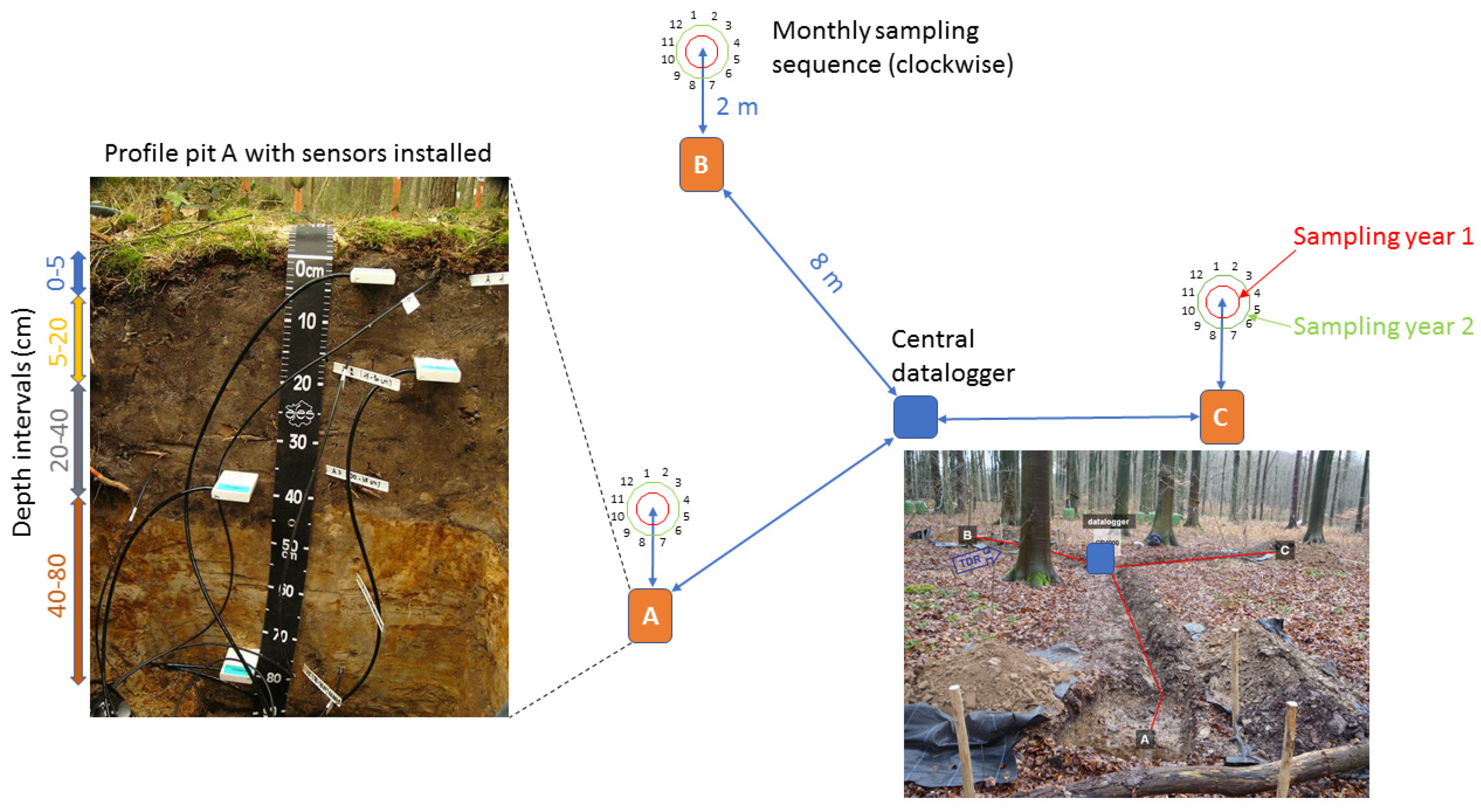
2.2. Monitoring Equipment: Soil Moisture and Temperature Sensors

The volumetric soil water content is measured at four depths using Campbell CS616 soil water reflectometers (FDRs). Each FDR sensor consists of two stainless steel rods (300 mm long, 3.2 mm diameter, 32 mm spacing) connected to a printed circuit board. A shielded four-conductor cable is connected to the circuit board to supply power, enable the probe, and monitor the pulse output. The circuit board is encapsulated in epoxy. High-speed electronic components on the circuit board are configured as a bistable multivibrator. The output of the multivibrator is connected to the probe rods which act as a wave guide. The travel time of the signal on the probe rods depends on the dielectric permittivity of the material surrounding the rods and the dielectric permittivity depends on the water content [20]. Digital circuitry scales the multivibrator output to an appropriate frequency for measurement with a datalogger (in our case a Campbell Scientific CR1000). The sensor output is essentially a 0.7 V square wave with frequency dependent on water content. The probe output period average (PA) ranges from about 14 microseconds with rods in air to about 42 μs with the rods completely immersed in tap water. A calibration function, which needs to be monotonically increasing, converts output period (PA) to volumetric water content (θFDR) predicted by the sensor. The probe output period (PA) was measured by a special CS616 data logger instruction and stored in the loggers’ memory as raw data.
Campbell Ltd. [20] provides standard manufacturers’ calibration functions, valid for all soils with a bulk electrical conductivity < 500 µS/cm and a soil bulk density < 1550 kg m−3:
Linear model θFDR = −0.4677 + 0.0283PA
Quadratic model θFDR = −0.0663 − 0.0063PA + 0.0007PA2
where θFDR being the measured volumetric water content expressed as a fraction (m3 m−3), PA the period average (in µs) as uncorrected sensor output.
The manufacturer reports an error in measured θFDR caused by the temperature dependency of the CS616 sensor, and provides the following correction equation to be applied to the uncorrected sensor output:
PAc = PA + (20 − ST) ∗ (0.526 − (0.052PA) + (0.00136PA2))
where PAc is the temperature corrected period (in µs), ST the soil temperature (°C) at the time and depth of the PA measurement. The coefficients of the standard linear (LM) and quadratic model (QM) given in (1) and (2) are also applied when using PAc instead of PA.
Soil temperature was measured using BetaTherm 100K6A Thermistor (model T107, Campbell) with a measurement range between −35 °C and +50 °C and with an interchangeability error of <±0.2 °C within the 0–60 °C range. According to the manufacturer and in a “worst case” situation, all errors add to an accuracy of ±0.4 °C within the range −24 °C to 48 °C and maximally ±0.9 °C within the range −38 °C to 53 °C.
Three dedicated profile pits were dug in spring 2010 and soil material was layerwise temporarily on-site stored till the pit was ready to be closed again, layerwise with exactly the same soil material. Prior to installation of the sensors, a soil profile description of the pedogenetic horizons was performed and soil core samples were taken at the fixed depth intervals 0–10, 10–20, 20–40 and 40–80 cm, yielding the data in Table 2.
CS616 sensors were carefully introduced horizontally in the wall of these soil pits (Figure 1). A fork hole with a dummy and level was applied to assure good contact of the rods with the soil following the guidelines of [13]. Through the horizontal installation of the 30 cm rods in order to determine vertical water fluxes, soil water content is ‘averaged’ over at least this length at the specific depth reducing small scale soil variation and capturing possible vertical preferential flow. Ruelle et al. [13] state that a horizontal buried probe at a particular depth will give the mean soil water content at that depth ± approximately 1.5 cm. Sensors were inserted at 4 depth intervals: 0–5 cm, 5–20 cm, 20–40 cm and 40–80 cm maximally overlapping the sampling depths of the long-term Level II soil monitoring program (Table 2) in order to relate physico-chemical data with time series of soil water dynamics for each layer.
At each site, the CR1000 datalogger was situated in the middle of the triangle formed by the profile pits A, B, and C (Figure 1), limiting the cable length between CS616 probe and logger to maximum 10 m. The T107 temperature sensors were installed at Pit A only (at all four depths) and at least laterally 10 cm away from the CS616 probe to avoid interference. The soil temperature readings of pit A were applied for possible temperature correction in the other pits. After installation of all sensors, the wiring holes were carefully covered with soil and the profile refilled layerwise. All sensors have continued operation since 2010, whereas some of the central CR1000 data loggers required periodical revision or replacement.
The accuracy specifications mentioned by the manufacturer for the θFDR measurement using the CS616 probes is based on laboratory measurements in a variety of soils and over the water content range air-dry to saturated. The soils were typically sandy loam and coarser. The CS616 accuracy is ±0.025 m3 m−3 using standard calibration with bulk electrical conductivity ≤ 500 µS cm−1 and soil bulk density ≤ 1550 kg m−3 in a measurement range from 0 to 0.50 m3 m−3. Resolution (i.e., the minimum change in the dielectric permittivity that is reliably detectable) is better than 0.001 m3 m−3. Precision or repeatability of the θFDR measurements in the same soil material is also better than 0.001 m3 m−3. Probe-to-probe variability ranges from ±0.005 m3 m−3 in dry soil to ±0.015 m3 m−3 in a typical saturated soil [20].

2.3. Soil Sampling and Analysis

For in situ calibration of the FDR sensors, monthly sampling during the period March 2015–March 2017 for bulk density and gravimetric soil moisture was performed using an Edelman- and Riverside auger and Kopecky steel cylinders of 100 cc (5.3 cm diameter; 5 cm of height). Since none of the soils are stony nor contain coarse fragments, this method is adequate for both the assessment of bulk density, gravimetric and volumetric water content. These core samples were taken using a closed ring holder (Eijkelkamp, Giesbeek, The Netherlands) loaded with the steel cylinder. The exact sampling depths are listed in Table A2. On the WIJ and GON plots the forest floor was >5 cm thick and FDR sensors were installed in the forest floor (OFH layer) of the B and C profiles. Hence, volumetric sampling was carried out in OFH layers as well.
Immediately after sampling and recording of the ring ID, the Kopecky cylinders were sealed with plastic covers (top and bottom) to prevent moisture loss, stored in an extra plastic bag and transported in a cooled box to the lab. Monthly sampling of the three soil profiles per site (4 sampling depths) was performed clockwise in a circle with a radius of 0.5 m from the reference point located 2 m north of the sensors (Figure 1). The sampled vertical profiles were about 25 cm apart from each-other. So, all core samples were taken between 1 and 3 m from the FDR sensors. This distance was required in order to avoid direct damage or interference with the active FDR and soil temperature sensors (and cabling), or indirectly by disturbing the local soil water distribution or preferential flow over the profile by monthly coring and sample extraction. We hereby assumed that the soil water content in the same soil layer was similar ~2 m away from the FDR sensor.
Following sampling, the borehole was carefully refilled and a bamboo stick was left in the last sampled borehole as an indicator for the next sampling. Care was taken not to disturb (compact) the soil too much when sampling the soil, especially on the future sampling locations. The second-year sampling was carried out in a circle with a radius of 1 m from the reference point (Figure 1, green circle).
The core samples were processed in the laboratory. Their wet/moist mass was determined prior to drying in a ventilated oven at 105 °C until constant mass, which was maximally one week for all soils. Then dry bulk density (ρbKop) was determined as oven dry mass per unit volume and gravimetric moisture content quantified. Volumetric water content was computed by multiplying gravimetric moisture content with the ρbKop of the sample. Sampling characteristics for all 5 sites are listed in Table 3. Overall, 1512 cores were processed to compile ρbKop and θv values for the calibration dataset.

2.4. Calibration Dataset

For all five sites, a calibration dataset was assembled with the attributes listed in Table 4.
After final calibration we added the corresponding recalibrated FDR measurements to the datasets (Downloadable from Supplementary material).

2.5. Statistical Evaluation

All statistical processing, evaluations and graphics were performed in the R environment, using R version 4.1.0 [29,30] in R Studio v1.3.1073. For time series manipulation and analysis, we used package xts v0.12.1. Evaluation of models was performed both for their relative and absolute quality. Relative model selection among candidate models was evaluated using the Akaike Information Criterion (AIC) corrected for small sample sizes (AICc) using the AICcmodavg package v. 2.3-1 [31]. The AICc weights for each model are given and the evidence ratios (ER) quantifying the amount of support in favor of a model relative to a competing model. Absolute quality of models was judged using a set of complementary validation indices of their predictive quality by comparing their predicted Pi with observed (reference) values Oi (Equations (4)–(8)). R2p is the prediction coefficient of determination informing the explained variance of the model (4), MPE is the mean prediction error or bias (5), SDPE is the standard deviation of the prediction error or noise (precision) (6), RMPSE is the overall model prediction error or model accuracy (7) and is the general closeness of agreement between the FDR output measurement (θFDR) and the reference observations (θv). RMSPE is the square root of the mean square prediction error (MSPE). For large n, MSPE equals the sum of MPE2 (bias) and SDPE2 (noise) as shown in Equation (8). With effective calibration the MPE (bias) is removed and the precision component of accuracy dominates.
R p 2 = [ cov ( P i , O i ) ] 2 var ( O i ) var ( P i )
MPE = 1 n i = 1 n ( P i O i )
SDPE = 1 n 1 i = 1 n ( ( P i O i ) MPE ) 2
RMSPE = 1 n i = 1 n ( P i O i ) 2
MSPE = 1 n i = 1 n ( P i O i ) 2 = MPE 2 + n 1 n SDPE 2
The revised index of agreement (dr) is dimensionless and bounded by [−1, 1] with 1 indicating perfect agreement [32]. Principal component analysis was applied using the R prcomp function, with data centered and scaled. The ggbiplot v.0.55 package was used to generate biplots using ggplot2 in order to plot both the position of each sample in terms of the principal components together with the initial variables mapped as vectors. In order to evaluate the importance of soil variables on the RMSPE, a generalized boosted regression tree model was built using the R package gbm v.2.1.8 with a gaussian distribution and following parameters: n.trees = 10,000, shrinkage = 0.01 and an interaction.depth = 4. The relative influence of each predictor, i.e., the reduction of squared error attributable to each variable, was used to select the most important ones for explaining RMSPE. Possible interaction was evaluated using the Friedman’s H-statistic which is on the scale of [0, 1] with higher values indicating larger interaction effects.

3. Results

3.1. Validation of FDR Measurements

3.1.1. Reference Dataset

The summary statistics of the reference dataset used for calibration are presented in Table A3. On the plots WIJ and GON, the upper FDR sensors were located in the forest floor layers (OFH) of B and C profiles, while in mineral topsoil (Ah layer) for the A profile. Hence, bulk samples for reference θv were taken in the same OFH layers (n = 47 in WIJ and n = 50 in GON) and the remaining in M01 layer of the A profiles. Local spatial variation in OFH thickness caused some reference samples to be more mineral than organic and vice versa. Therefore, we considered reference samples having a ρbKop < 850 kg m−3 (threshold derived from [29]) as part of OFH layers, and above this threshold as M01. On RAV and HOE, two reference Kopecky samples qualified as OFH samples, whereas none in BRA topsoil samples.
Over the total calibration period raw FDR sensor output ranges from 20.5 to 34.1 µs in the OFH layers, and from 17 to 41.9 µs in mineral layers, covering the full range reported by the manufacturer [20]. Note that on the plots WIJ and GON, neither significant differences in period means nor ranges were found between the FDRs in the OFH and those in the mineral layer (M01) for the same site. However, the observed mean period was lower on the sandy site WIJ compared to the heavier textured GON site (Table 1). Overall, the PA values are lower in the sandy soils (WIJ, RAV and BRA) than in the silty and clayey soils of GON and HOE. Within sites, the mean PA values differ significantly among depth layers as shown by the 95% confidence interval of the means, which can be attributed both to specific soil layer properties and a possible sensor effect.
Each sites’ soil temperature was sensed in the A profile only. Mean annual soil temperature was roughly above 10 °C on the sandy sites, and slightly lower on the heavier textured soils, but this difference is neither significant between sites nor between soil layers within the sites for the reference dataset. However, the range is wider in the topsoil layers, especially in the forest floor (OFH) which may warm up to 25 °C. In subsoil layers, the amplitude of the temperature fluctuations is reduced due to the well-known damping effect. Soil bulk density, known for its significant effect on dielectric permittivity, is significantly smaller in the OFH layers compared to the mineral layers (M01–M48). In the mineral soil profile of each site, ρb generally increases with depth. Lowest ρb values are found in GON and highest in HOE (Retisol), but also elevated values in the Arenosols (RAV and BRA).
At the WIJ and GON sites, the mean gravimetric soil water content (θm) in the OFH layers is more than three times θm in the mineral soil, clearly showing that forest floor layers can hold more water than their dry mass compared to mineral layers generally storing less than 50% of their mass. On all sites, mean θm significantly differs by layer with higher mean moisture contents in the 0–10 cm topsoil (M01) due to elevated contents of organic matter. Depending on the depth of the groundwater, perched water table or subsurface flows, mean θm can rise again in the M48 layer. Volumetric soil water content (θv) is greatest in the OFH up to 0.62 m3 m−3 while maximally 0.52 m3 m−3 in M01 layers. Again, significant differences in means are found by mineral layers within sites and between sites, justifying the need for multiple moisture sensors. The observed means and ranges of θv indicate clearly that RAV and BRA are the driest plots (0.05–0.06 m3 m−3 in dry periods), WIJ can store more soil water in its organic-rich sandy soil compared to HOE in the silt-loam soil, while highest mean θv values are observed in GON (0.38–0.47 m3 m−3) due to the perched water table above the clayey substrate (Table 1).
For all plots, layer specific graphs are presented in S1 to S5 showing the temporal variation of sampled soil water content in the three profiles, the corresponding FDR response (Period) and their linear relationships. These graphs clearly show variable types of relationships among layers, and within layers (especially topsoil layers) distinct linear relationships between the profiles. For WIJ (Figure A1 and Figure S1) calibration will be difficult in the topsoil due to high scatter of calibration data (mix of M01 and OFH layers) and limited slope of the linear models. For deeper mineral layers of the WIJ plot with a more limited range in water content, adequate calibration is more feasible, and similar slopes indicate higher correlation between profiles even suggesting that one single calibration function per layer would be feasible. Other hard to calibrate profiles are profile A of layer 1 in RAV and profiles B and C in GON layer 4. Overall, these graphs indicate that layer and profile specific calibration is preferred using reference measurements taken close to the sensors.

3.1.2. Calibration Testing

Based on the calibration dataset, a two-step testing approach was adopted. First, we validated the standard models suggested by the manufacturer by simply relating the measured θv at a specific moment with the observed output period of the FDR sensor at that moment, for each of the 60 soil layers. In Figure 2a these observed data-pairs are plotted along with the standard function for the M12 layer of profile B on the HOE site. Clearly the standard function underestimates the measured θv (negative bias of −0.0534 m3 m−3, data in Table S5). In the second step, we recalibrated the model in order to remove the bias, and used this recalibrated model for predicting θFDR using the continuous FDR output period values. Note that with calibration the accuracy improved (RMSPE decreased from 0.057 to 0.019 m3 m−3) and the index of agreement substantially increased from 0.67 to 0.91. Figure 2b illustrates that the monthly measured real soil water content is much better predicted when the recalibrated function is applied.
The standard response remains permanently below field capacity whereas the recalibrated response during winter is situated between θs and θfc as expected. In summertime standard response drops below θpwp in contrast to recalibrated response and the calibration measurements.
Note that the calibration measurements on the HOE plot started in February when soils were above field capacity, then followed a drying phase until September and a fast-rewetting phase in October/November. To improve calibration for the HOE plot, more calibration pairs would be beneficial for θv between 0.25 and 0.35 m3 m−3, roughly situated between May and the end of November.
For each plot, layer and profile, graphs as in Figure 2b were produced to illustrate all calibration results of this study (Figure A1, Figure A2, Figure A3, Figure A4 and Figure A5), with indication of measured θfc and θpwp.

3.1.3. Validation of Standard Functions

For all plots, profiles and layers, standard calibration functions (Equations (1) and (2)) were applied and the coefficients of determination (R2) and predictive quality indices are listed in Tables S1–S5.
The standard linear (LM) and quadratic models (QM) generally explained the measured topsoil water content rather poorly, indicated by R2 as low as 0.005 in OFH layers of the WIJ site and explaining just 10 to 50% of the variance in mineral soil layers. With increasing depth, the standard calibration functions approximate the measured water contents slightly better. Figure 3 displays the positive or negative bias (MPE) and total prediction error (RMSPE) of the standard linear and quadratic functions when predicting the measured θv.
In general, the quadratic standard model generates a greater bias and total prediction error compared to the linear model. A paired t-test of all profiles and layers reveals that when the standard LM is used the bias is 0.015–0.019 m3 m−3 smaller compared to the QM for all plots but GON (Table 5). On the latter plot a positive bias (i.e., overestimation of θv) was observed attributed to the clayey subsoil layers (Figure 3). As expected, the random error (SDPE) does not differ significantly between standard LM and QM. The resulting overall prediction error is significantly smaller when using the standard LM, and its index of agreement is significantly greater.
On the WIJ, RAV, BRA, and HOE plots a predominantly negative bias was found, especially in the topsoil: up to 0.16 m3 m−3 in mineral (M01) and up to 0.32 m3 m−3 of θv in OFH layers was underestimated (Tables S1–S5).
For almost all layers the allowable measurement error threshold for θv of 0.03 m3 m−3 is exceeded except for two M48 layers in RAV, and two M48 layers in HOE. So, for only 4 out of 60 layers the (linear) standard function predicts θv according to the required level of accuracy.
The mean total prediction error is greatest for the GON plot (RMSPE = 0.17 m3 m−3) and smallest for the RAV plot (0.07 m3 m−3). The RMSPE is similar for BRA and HOE. The greater overall prediction error on the sites WIJ and GON is mainly due to the large prediction errors of the OFH layers (Figure 3). If we omit the values for OFH, the mean RMSPE for WIJ becomes 0.09 m3 m−3 whereas it remains high (0.17 m3 m−3) for GON here due to the high estimation errors in the clayey substrates.

Temperature Correction

Prior to the use of the standard LM and QM, a temperature correction (TC) of the PA signal was performed using Equation (3), and compared to the same model without TC (Table 6). Results show that TC reduces the MPE (bias) significantly for both model types, but has a small to insignificant impact on the precision error, except for WIJ.
For the WIJ plot, overall accuracy as indicated by RMSPE and index of agreement improved significantly, but for the other plots the improvement was negligible. Hence, temperature correction for the standard functions may help in reducing prediction bias.
When evaluating the overall RMSPE of standard models with temperature correction, only the predicted θv of the M48 layers in RAV was not exceeding the allowable error of 0.03 m3 m−3, so for only 2 out of 60 layers water content was predicted accurately.

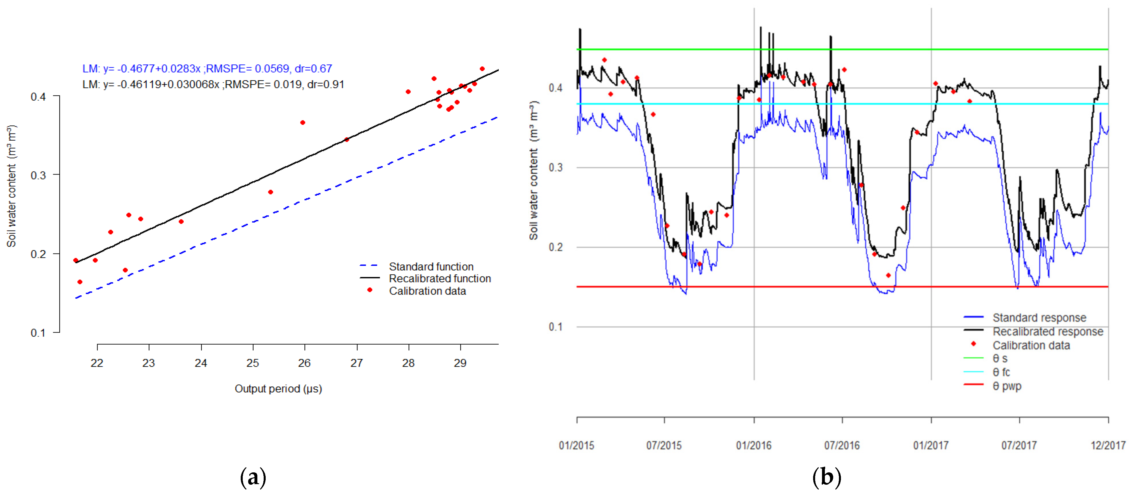
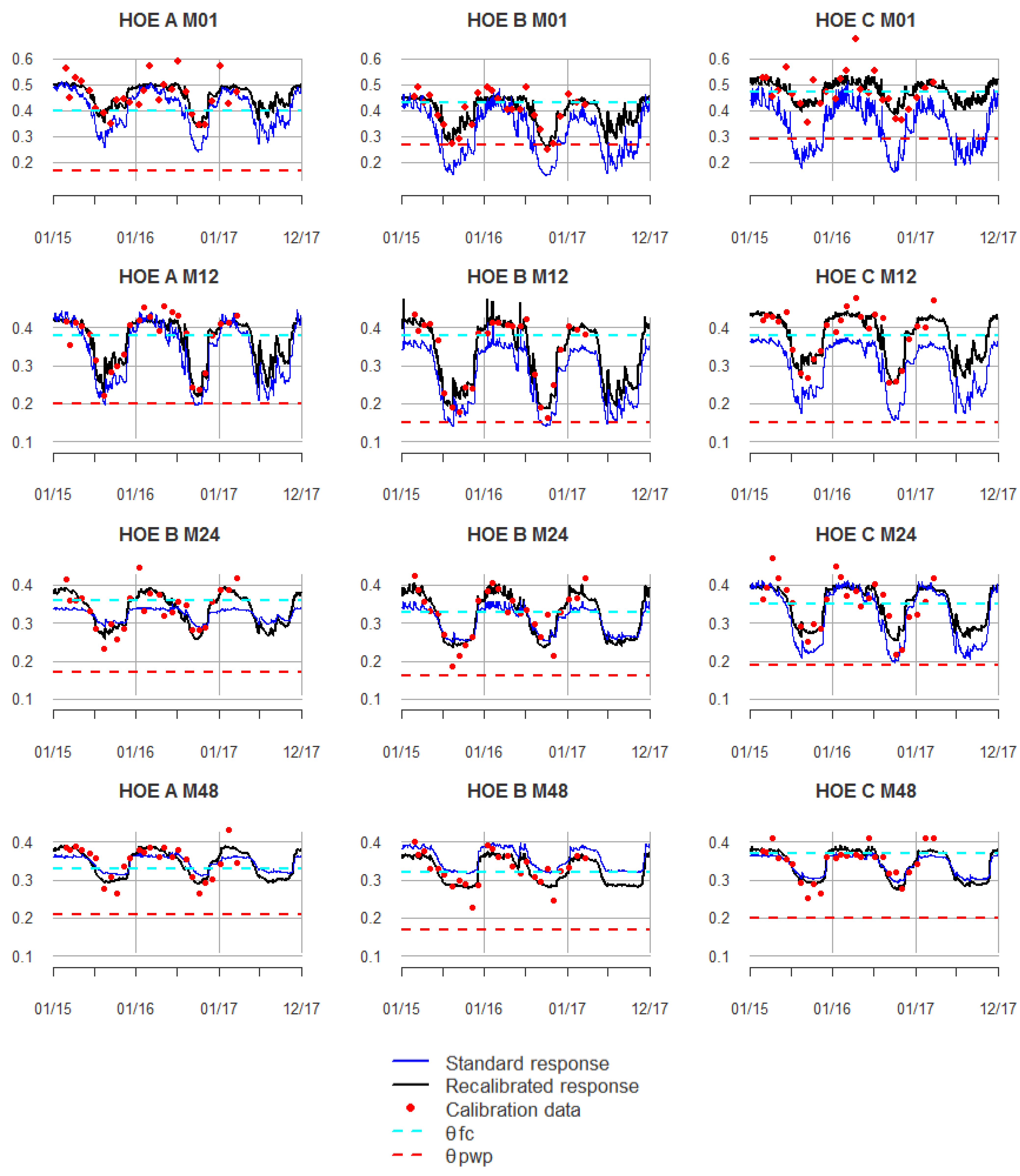
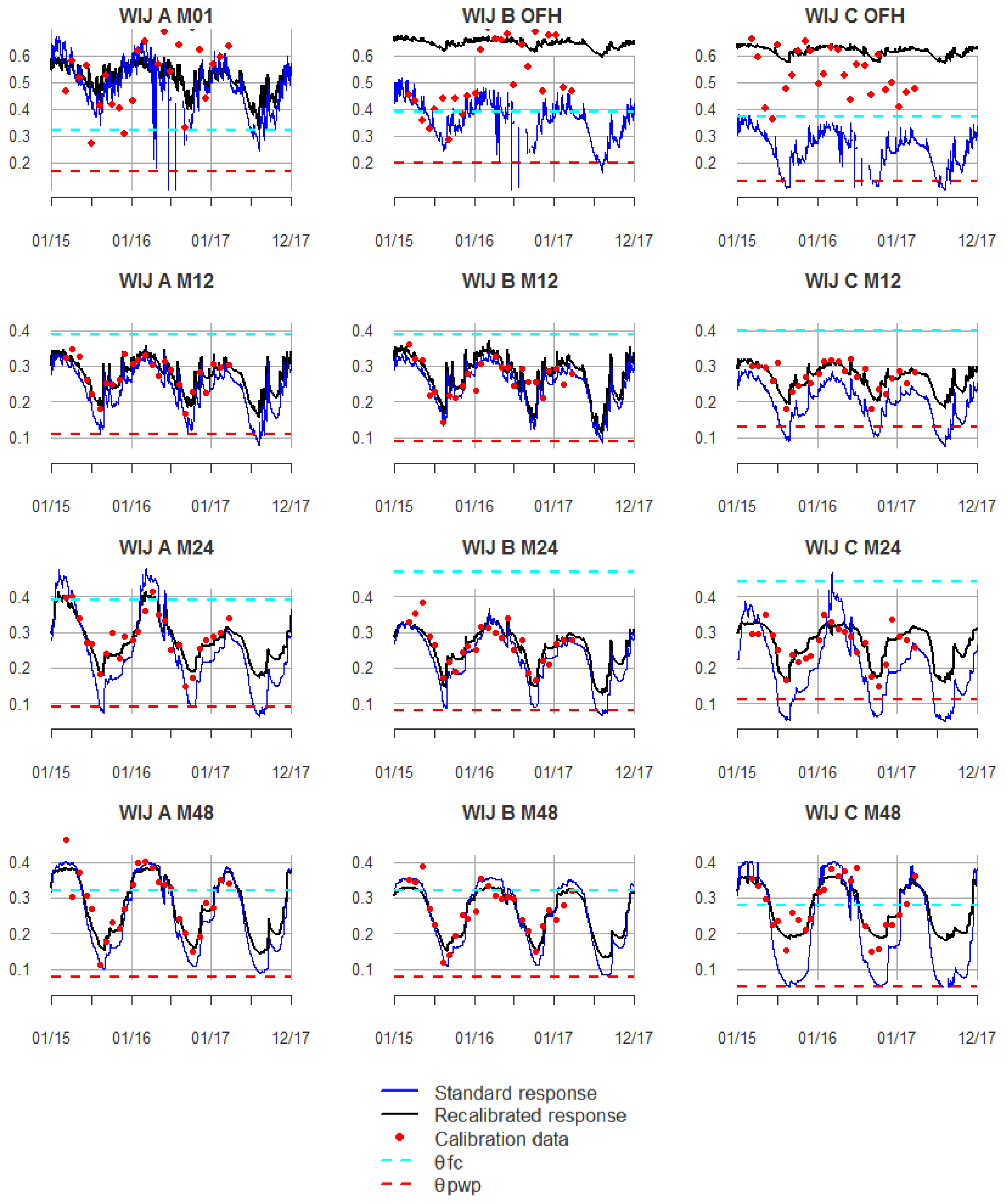
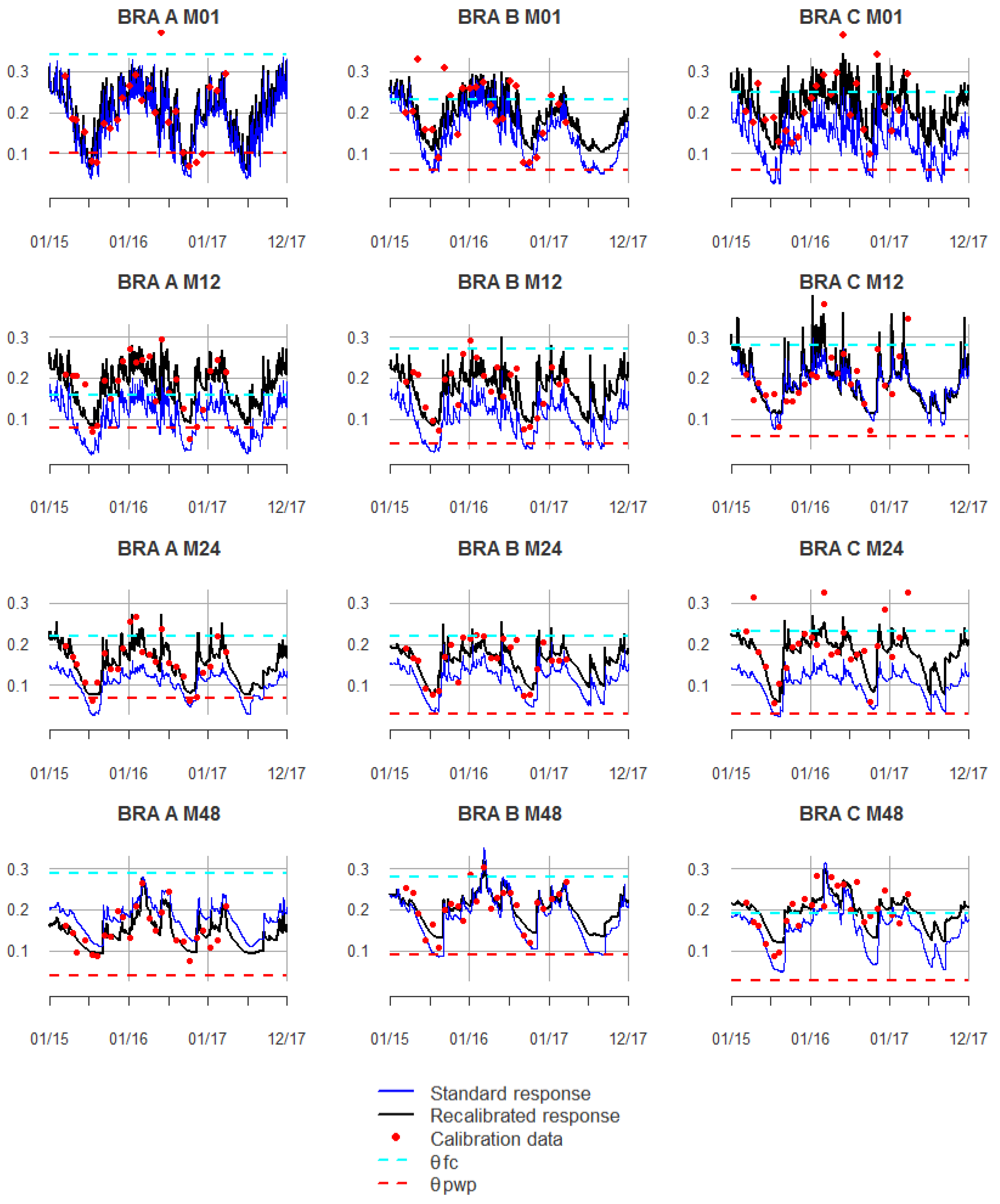
3.1.4. Validation of In Situ Recalibrated Functions

For each layer four candidate recalibration models (LM and QM, with and without temperature correction, denoted LMTC and QMTC), are compared relatively to one another and the best and second-best models were selected based on lowest AICc value (Table A4). For 32 out of 60 layers, the simple LM proved to be the most parsimonious model and was supported over the LMTC or QM. Using the AICc, a LMTC was selected as the best model for 23% of all layers, more frequently than the QM (13% of all layers) and QMTC (10% of all layers). Evidence ratio’s (ER) between the best and second-best model ranged from 1.01 (equally well) to 22.8 times better. Generally, the best model in the topsoil had no temperature correction which is remarkable for the layer where variation in soil temperature is greatest.
By definition, recalibration of the standard functions eliminates bias so that overall prediction error is mainly determined by the SDPE (precision) composed of errors attributed to (short distance) spatial variation, sampling errors and random measurement error. Figure 4 shows the calibration gain of the overall prediction error for the best standard (i.e., with highest dr) and recalibrated functions for all plots.
Hence, compared to the standard functions, recalibration lowered the overall prediction error with a factor 1.8 (RAV) to 2.8 (GON). When comparing plots, the mean RMSPE is greatest at the GON plot, still double the allowable error of 0.03 m3 m−3 while on HOE the mean RMSPE equals the threshold while the means of the other plots are in between. For GON, not a single layer meets the threshold, whereas in HOE only three layers are exceeding the threshold when using the best recalibrated model.
Apparently, accurate prediction of θv is most challenging for topsoil layers, whether they are organic (OFH) or mineral (M01) or most likely organo-mineral, with organic contents and bulk densities in between pure organic and mineral materials (Figure A1). However, some subsoil layers, such as M48 in GON show high prediction errors. From Figure A4 it is clear that the recalibrated response for the B and C profiles in the M48 layer shows almost no variation in contrast to highly variable gravimetric measurements.
We carefully checked whether all quadratic calibration models (QM and QMTC) selected as best models based on AICc (Table A4) were monotonically increasing functions (i.e., increasing output period should physically relate to higher soil water content). Five functions (WIJ-B-M12, RAV-C-M12, GON-B-M12, GON-C-M12, and GON-C-M48) did not meet this requirement. For example, in the GON-C-M12 layer, the QMTC calibration function increased until a temperature corrected period of 31 µs and decreased afterwards (Figure 5). We replaced this function by the LM (selected as second best by AICc in Table A4), hereby explaining even less variance (27% to 12%) but with a more plausible calibration function, though a greater prediction error.
For the heavy-clay subsoil M48 layer in GON C profile, no adequate monotonic function could be constructed, meaning that no calibration of that FDR sensor in a layer with ~47% clay was feasible with the given calibration dataset (Figure A4).

3.2. Explaining the Prediction Errors at the Plot Scale

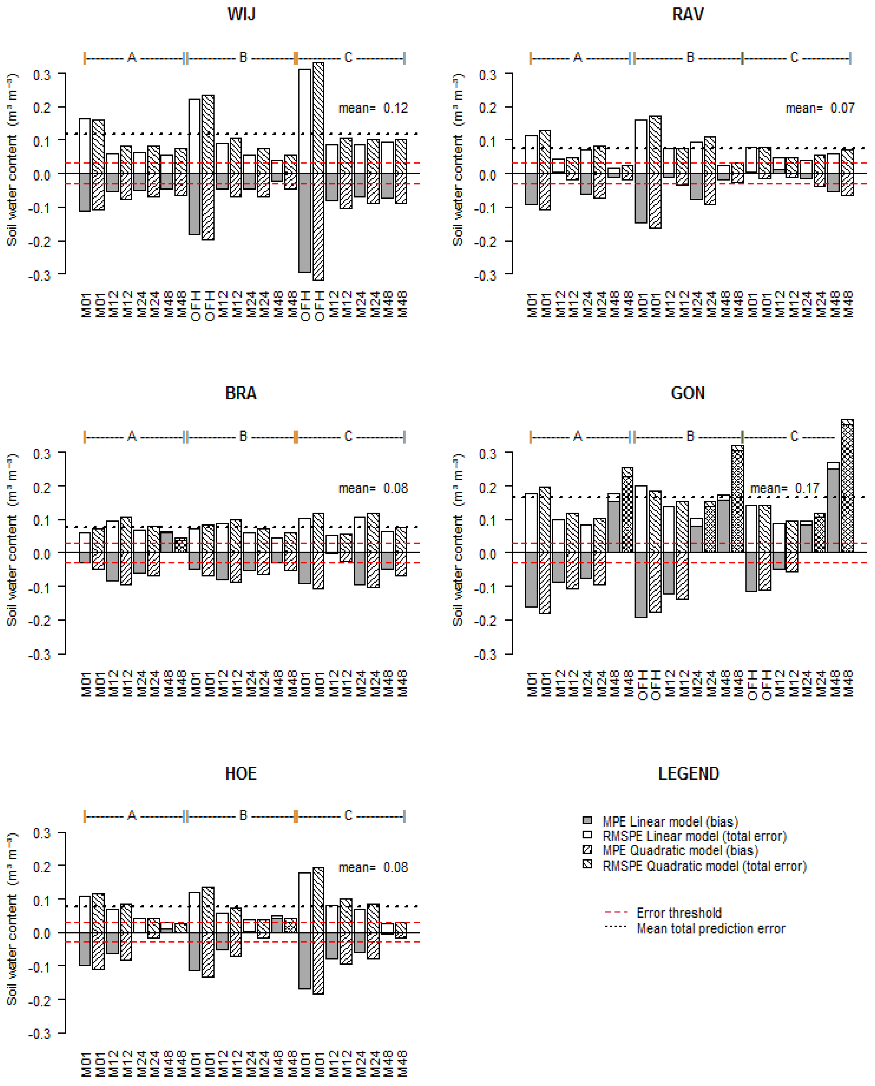
3.2.1. Contributors to Bias

The principal component analysis (PCA) biplot in Figure 6 is based on the estimated bias (MPE) of the standard LM along with the soil properties of each layer of the 5 sites (Table 1 and Table 2). The first 2 principal components (PC1 and PC2) explain 65% of the variance, PC3 and PC4 add 12 and 9% and these are mainly determined by EC and pH-H2O, respectively. The factor loadings of PC1 are dominated positively by ρbKop, and negatively by CEC, θs, TOC and TN. Bias is mainly contributing to PC2, strongly associated with Clay content and soil depth, all having negative factor loadings. Indeed, in topsoils (M01 and OFH) we mostly found a negative bias (underestimation of real θv) while a positive bias was generally found in subsoils, especially when they are clay rich. The impact of depth justifies separated calibration by depth layer.

3.2.2. Contributors to Overall Error

When the bias is eliminated by in situ calibration the overall prediction error (RMSPE) is dominated by the precision error. In Figure 7 the PCA clearly indicates that on PC1 the RMSPE is closely and positively associated with TOC and TN and negatively correlated with ρbKop and Depth. The lower the ρbKop, the higher RMSPE, and this is extremely visible in the OFH layers, which obviously have a high TOC and TN content. PC2, explaining still 22% of the variation, is mainly determined by texture fractions Clay, Silt and Sand, but is rather uncorrelated with RMSPE. Conversely, Clay and Silt are associated with greater values for Ɵfc and Ɵpwp.
The PCA clearly shows that BRA and HOE are more homogenous sites in terms of soil properties as indicated by smaller ellipses, and independently from the fact that they are texturally very different from each-other, have low overall prediction errors. Conversely, WIJ and GON have high variation in soil properties and thick OFH layers leading to high overall RMSPE especially for the organic layers low in ρb.
When we build a generalized boosted regression tree model to predict RMSPE based on the layer specific soil properties (Table 1 and Table 2), the relative influence of the predictors is given in Table 7. Two predictor sets were applied, Set 1 using ρbKop (Table A3), and Set 2 using ρb as listed in Table 1.
Upon using the first set, bulk density in the sampling rings is clearly the major predictor and has higher influence than depth, θs, clay fraction, and all other soil variables. When replacing ρbKop by ρb, relative influence decreases and the saturated soil water content takes over as the major predictor. Since θs is inversely correlated with ρbKop (Figure 7) this is no surprise. Samples with greater θs and consequently lower ρb have more macropores, allowing air to enter and influencing the dielectric permittivity and PA output. Two-way interactions between predictors as indicated by Friedman’s H-statistic are all below H = 0.11 (between depth and θr) and therefore negligible.

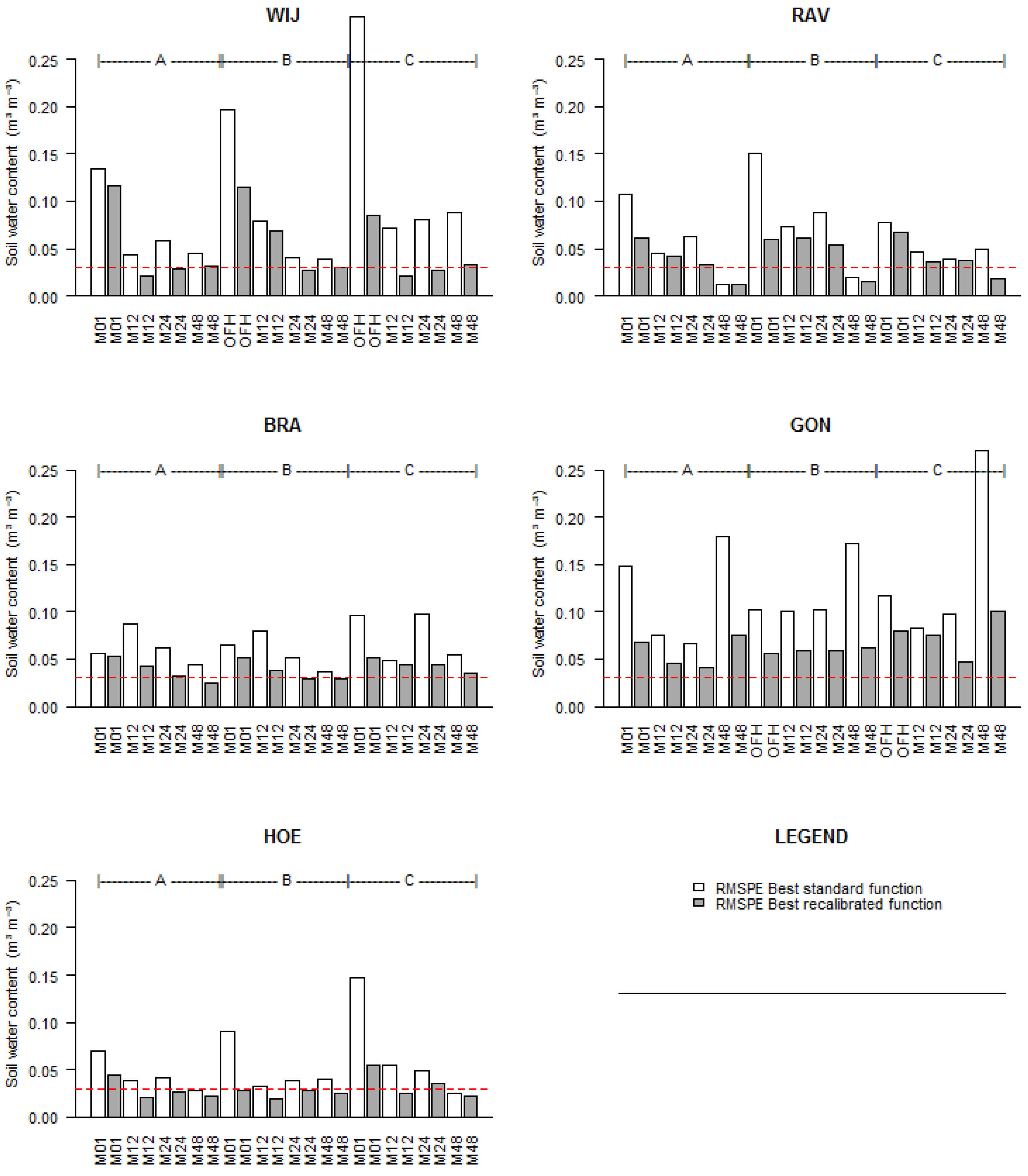
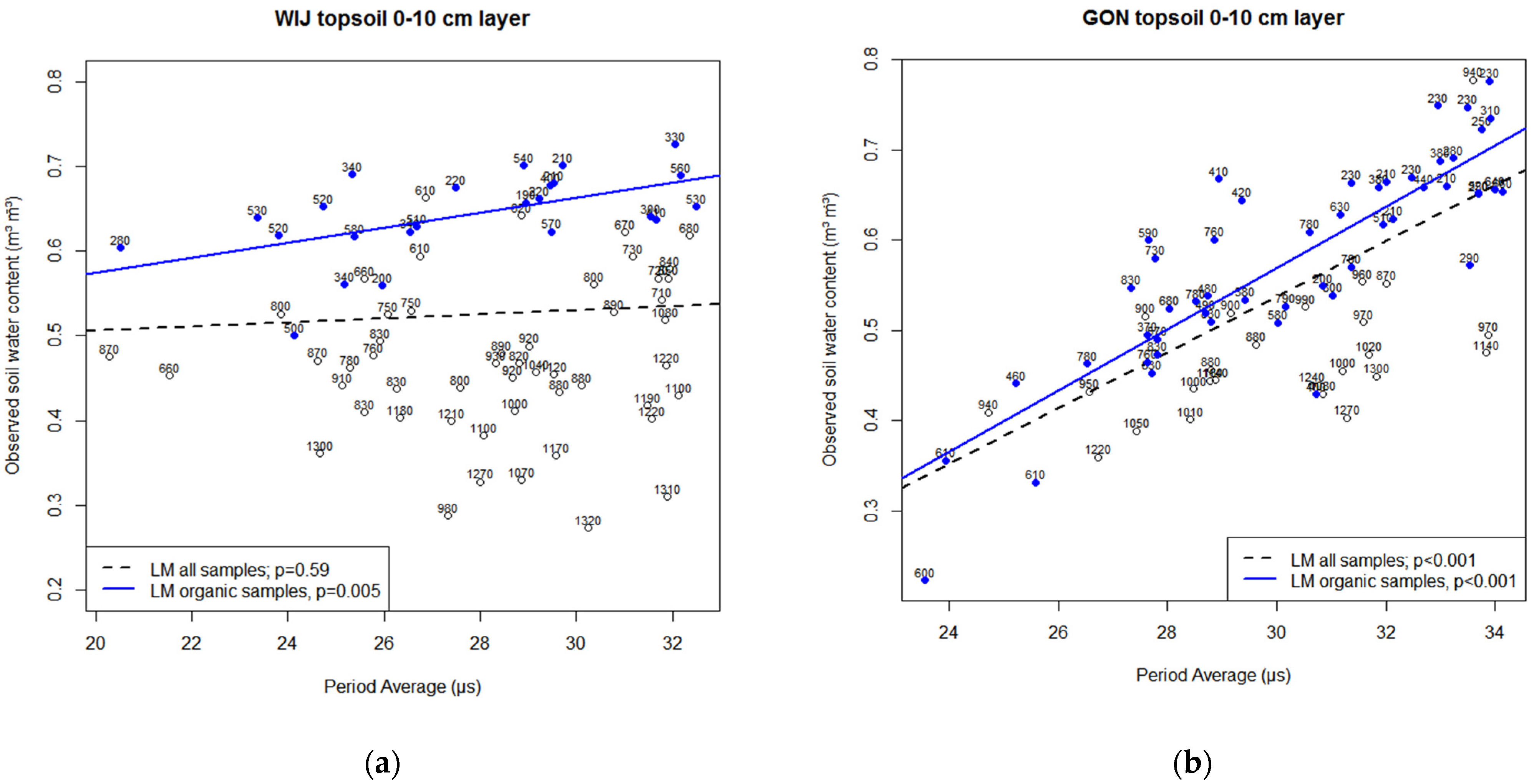
3.3. Improving the Prediction Errors in Organo-Mineral Topsoil Layers

The statistical evaluations clearly indicate that accurate prediction of θFDR is most challenging for the topsoil layers due to high natural variability of ρb and organic carbon in the organo-mineral layers.
For the plots WIJ and GON where the FDR sensors are installed in the OFH layers (B and C profiles), accurate calibration is jeopardized by the high variability of the reference samples taken each month. This can be seen from the scatterplot of the WIJ site in Figure 8a. With high PA values (PA > 31 µs) of the sensor, θv may range from 0.31 to 0.73 m3 m−3 and ρb from 300 kg m−3 (pure organic matrix) to 1310 kg m−3 (mineral matrix). It is also clear that the lower the ρb (and hence more organic the reference sample), the more soil moisture (θv) may be stored, often more than 0.5 m3 m−3 compared to mineral samples (ρb > 850 kg m−3) holding less than 0.5 m3 m−3 (see θs values in Table 2).
Selecting from each WIJ profile (max 25 calibration pairs) only the organo-mineral samples by their ρb value (i.e., ρb < 850 kg m−3) yields too few samples for adequate calibration per profile. Therefore, we pooled all topsoil samples from the three profiles of the WIJ plot (n = 75 samples). When calibrating a LM the slope of the model was not significantly different from 0 (Figure 8a). When subselecting organo-mineral samples with ρb < 850 kg m−3, a LM based on n = 47 paired observations was calibrated: θFDR = 0.320295 + 0.00971 PA, with R2 = 0.119, p = 0.0099 and RMSPE = 0.0745 m3 m−3.
Based on AICc criterion, QM, LMTC nor QMTC models performed better than the LM. However, when varying different thresholds for ρb, the best linear calibration model was found for organo-mineral samples with a ρb < 600 kg m−3, and parameters: ƟFDR = 0.39962 + 0.008767 PA, with R2 = 0.276, p = 0.005 and RMSPE = 0.0417 m3 m−3. The selected samples (n = 24) and calibration function are indicated in Figure 8a. Only one-third of the total number of calibration samples was selected, but this number resembles the 25 samples used for calibration of each individual profile.
Note that the overall prediction error lowered substantially from 0.1126 to 0.0417 m3 m−3. The resulting recalibrated response for the B and C profile can be seen in Figure A1. The moisture content remains high in the OFH layers compared to the A profile or underlying mineral layers of that plot.
The situation is somewhat different for the GON site (Figure A4), where combining all topsoil calibration pairs already leads to an adequate LM: ƟFDR = −0.38825 + 0.030858 PA, with R2 = 0.515, p < 0.001 but a relatively high RMSPE = 0.0785 m3 m−3 (Figure 8b). Here also some calibration samples had high ρb values (up to 1300. kg m−3) while others are as low as 200 m3 m−3. When selecting a subset of samples with ρb < 850 kg m−3 (n = 50) the best regression model was found, again a LM outperforming the other model types based on AICc) with parameters: ƟFDR = −0.45026 + 0.033966 PA, R2 = 0.716, p < 0.001 and RMSPE = 0.0591 m3 m−3. The selected calibration samples and LM are indicated in Figure 8b. Note that this calibration function is not performing better than the originally recalibrated one for profile B (RMSPE was 0.0553 m3 m−3 while the revised function yields 0.0591 m3 m−3 but better for the OFH layer in profile C that had a RMSPE of 0.0797 m3 m−3). Since the sensor is effectively located in organo-mineral layers, we replaced both by the new function (Table A5). The resulting time series for GON is presented in Figure A4. Here the seasonality of the moisture content of the OFH is much more pronounced than in WIJ, with expected higher moisture levels than in the M01 layer. Note that the Ɵfc was estimated for mineral samples, not for the OFH layer.

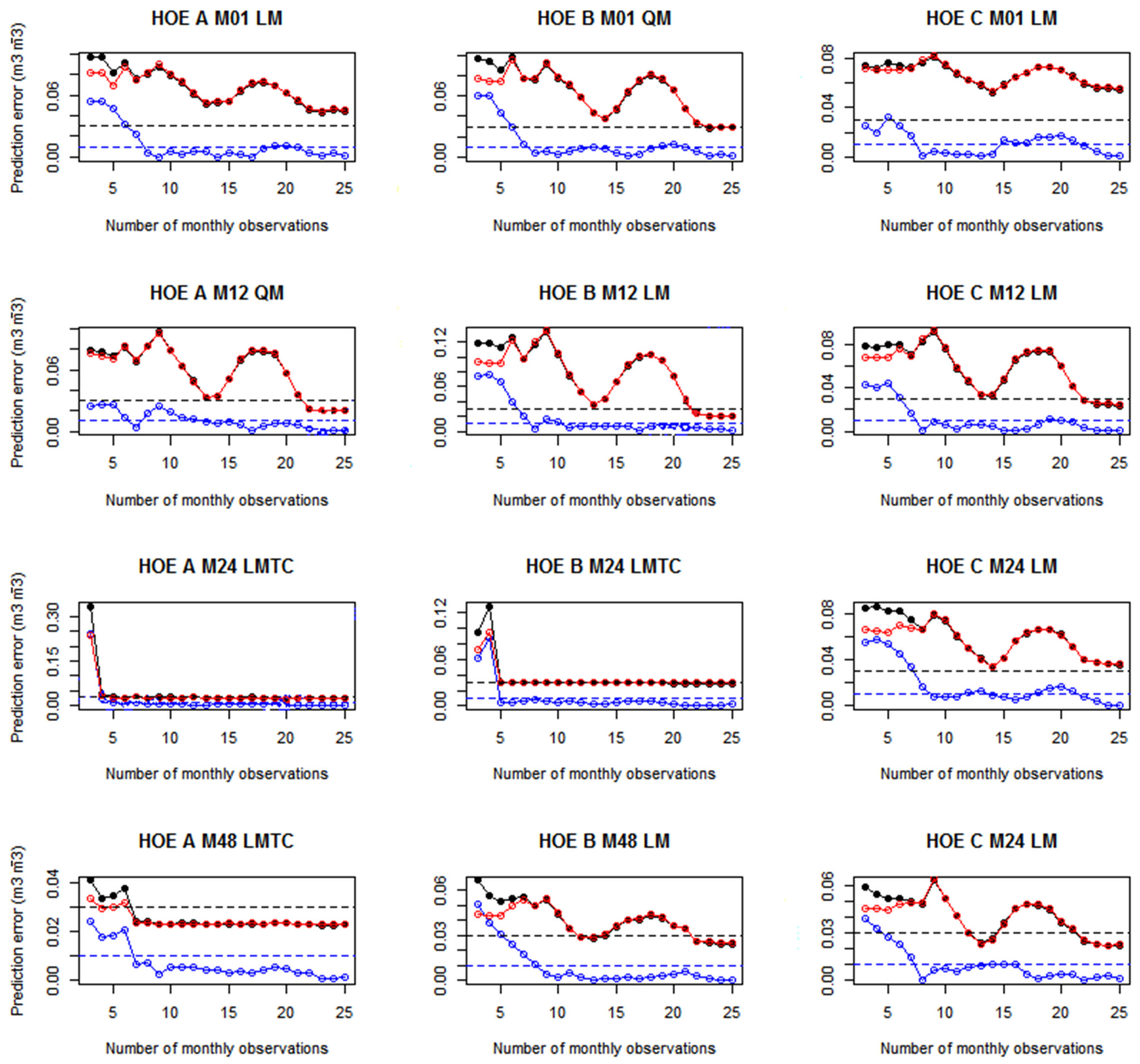
3.4. Requirements for Optimal Calibration

The practical question is raised how many field samples are required for adequate calibration of the FDR sensors. Figure 9 shows a simulation for the HOE site with the evolution of the overall prediction error (RMSPE in black), the bias (MPE in blue) and precision (SDPE in red) relative to an increasing number of calibration months, beginning from a three months period. Starting when soils are near field capacity (in February/March) extra calibration data is gained during spring and summer months when soils are gradually drying out. This substantially decreases the bias until August (i.e., eight months). Since the bias is eliminated by then, the overall error is converging with the precision error during this first calibration period.
We considered the bias as sufficiently eliminated when the MPE is continuously below a 0.01 m3 m−3 threshold (i.e., the maximal error of the gravimetric reference measurement). The number of months required for each plot, profile and layer is given in Table 8. It is clear that for all plots a longer calibration period is needed to remove the bias in the topsoil (19−24 monthly observations) compared to subsoil layers, although some special layers also require almost two years of calibration.
The precision error starts to decline substantially from 9 till 14 observation months, when soils are rewetting until field capacity in March, but raises again during the drying phase until driest conditions in August/September and declines again in the rewetting phase afterwards. For the M12 layers of the HOE site, the precision (and overall) error drops below the 0.03 m3 m−3 threshold after more than 22 observation months, but for the M01 layers in HOE and on the other sites much more than 25 observation months are required or will exceed a reasonable calibration period (see RMSPE Table A5). In that case, due to the high precision error (noise), reducing the prediction error will only be possible by increasing the number of sensors for these specific layers.
For those layers where the sensor’s precision error after calibration still exceeds the threshold of 0.03 m3 m−3, and assuming that the bias is near-zero and the observed precision error is of the same magnitude for other individual CS616 sensors used under similar (soil) conditions, the average measurement error can be reduced by the square root of the number of sensors installed in parallel in the given layer, following the classical central limit theorem.
For each layer, we therefore estimated the number of sensors required to reduce the maximum SDPE found in the three profiles of that layer (data from three individual sensors) to a measurement error below 0.03 m3 m−3. So, the most difficult calibration environment per layer will determine the number of sensors needed for averaging soil moisture measurements of that layer at the plot level (Table 9).
Table 9 suggests that the current number of three sensors is sufficient for all layers of the sites BRA and HOE. However, more sensors are required for the topsoils up to 20 cm of depth for WIJ and RAV, and also for the subsoil layers in GON, with up to 10 sensors in the clayey substrate if the required measurement accuracy has to be met.

3.5. Final Calibration Functions

The best performing calibrated functions with eliminated bias for each site and layer are presented in Table A5. These functions are applied to the respective FDR sensors of the LII plots to construct the ƟFDR time series and may be considered the end-product of this study. For the 60 layers examined, a linear model (LM) was the best choice for 58% of these layers and 27% of them a LM with temperature correction. Quadratic models seemed more appropriate for 10% (QM) and 5% (QMTC) of all layers. The resulting time series of all calibrated models for the 2015–2017 period is given in Figure A1, Figure A2, Figure A3, Figure A4 and Figure A5.
On average, calibration functions explained 56% (median 61%) of the total variance of the calibration dataset with a maximum of 96%, but also with no variance explained at all (R2 = 0.003) in the special case of extremely clayey substrates. The RMSPE ranges from 0.012 to 0.117 m3 m−3 with a mean of 0.043 m3 m−3 and median 0.041 m3 m−3. Hence, regardless of specific soil conditions, measurements of one sensor per layer will not suffice to predict Ɵv better than the 0.03 m3 m−3 accuracy threshold.

4. Discussion

4.1. Attainable Level of Predictive Accuracy

One of the fundamental questions of this study is the level of predictive accuracy, as indicated by the RMSPE, one can achieve using the CS616 sensor for θv measurement in various soil types compared to reference gravimetric sampling. Hignett et al. [11] estimated the RMSPE of the reference method to maximally 0.01 m3 m−3. The user manual [20] of the CS616 mentions that the factory standard calibration is accurate to ±0.025 m3 m–3 in the θv range of 0−0.50 m3 m–3 valid for soils with low bulk electrical conductivity ≤500 µS cm−1 and bulk density less than 1550 kg m−3. This conforms with all forest soil layers under study.
In Table 10 we compiled RMSPE values obtained with standard and revised functions in various studies for coarse to fine textured soils and organic layers using the CS616 sensors. From all mentioned studies it is clear that recalibration or correction for the specific soils significantly reduces the overall prediction error. The standard function provided by the manufacturer [20] generally performs best for sandy samples [1,10], but as clay content increases, larger prediction errors are found and soil-specific recalibration is absolutely required [1,3,4,6,7,9,11]. Most recalibrations or corrections are performed in the laboratory, since field-based calibration is challenging to perform for many users [10].
The RMSPE quality criteria set by [4] for a mean bias ± 0.02 m3 m–3 and RMSE < 0.035 m3 m–3 or a RMSE < 0.30 m3 m–3 for forest soils by [18] are rarely met, even after (re)calibration or correction.
Furthermore, revised calibration functions developed under controlled but limited laboratory conditions, are not always appropriate for field conditions [1,5]. In 2008, an international group of soil water instrumentation experts came to the conclusion that “all soil moisture sensors must be field calibrated in order to obtain reasonable accuracy” except conventional time domain reflectometry (TDR), which is accurate to ±0.02 m3 m–3 in most soils [11].
Most studies mentioned in Table 10 collected (large) volumetric field samples in containers and transported them to the lab in order to test a number of moisture sensors and compare the results using standard and revised functions. For practical reasons they calibrate their sensors during a drying phase [3] under controlled temperature and humidity conditions. In our in situ calibration approach we sampled over two years two drying phases and two rewetting phases (Figure 2b), accounting also for the real soil temperature variations associated with the moment and depth of sampling.
On the other hand, since gravimetric soil sampling is destructive and we cannot sample close (i.e., less than 1 m) to the sensors to avoid interference, we add spatial and sampling errors to our validation measurements. This set-up requirement is the major limitation of our in situ calibration approach, certainly since many forest soils tend to have a high small-scale variability of moisture influencing soil parameters. Most reference studies reported that the factory-based standard function underestimates the real moisture content, but under- or overestimation seems dependent on the soil texture. However, Varble and Chávez [4] found in the laboratory that the factory calibrated CS616 sensors overestimated θv by an average bias of 0.10 m3 m−3 in sandy clay loam, 0.03 m3 m−3 in loamy sand, and 0.24 m3 m−3 in clay loam. This is contrasting to [1] where negative biases and much lower values were found for the same texture classes. In our study we found that standard functions generally underestimated sand layers with MPE = −0.042 m3 m−3 and loamy sand with −0.053 m3 m−3 which is greater than these studies, but this might be related to our in situ sampling.
Dong et al. [1] corrected the standard functions with correction equations but the improvement was quite small: 0.011 m3 m–3 for sand to 0.002 m3 m–3 in loamy sand and 0.027 m3 m–3 in sandy clay loam. We believe that recalibration of the models is more effective than applying correction equations on poorly performing factory-based functions, and that only calibrations using in situ measurements can lower the effective bias substantially.
The standard functions (Equations (1) and (2)) provided by Campbell are found inadequate for clay and clay loam soils (Table 10), often overestimating θv. Varble and Chávez [4] reported the average RMSE of the clay loam samples (n = 65) as 0.289 m3 m−3 compared to 0.21 m3 m−3 for clays in our study. Using laboratory-based recalibration, they succeeded to eliminate bias and reduce the resulting RMSE below 0.021 m3 m−3 for the clay loam soil, an error reduction of 93%. In our study RMSE after in situ recalibration is still 0.076 m3 m−3 for clay samples, an error reduction of 63% (Table 10).
Veldkamp and O’Brien [7] tested heavy clay soils (60−80% clay) and found standard calibrated CS616 sensors to underestimate water content up to 0.15 m3 m−3. This is in contrast with our findings that clay soils are overestimated with the standard function, but clay mineralogy clearly differed between our studies. Instead of recalibrating the models for the clayey soils [7] developed a 3-phase mixing model for topsoil and subsoil separately and reduced RMSE for these clay soils to maximum 0.012 m3 m−3. (error reduction of 93%). This 3-phase mixing model, using a physical basis for the derivation of the calibration function, might be a good alternative for recalibration functions, especially for soils rich in clay and organic matter.
Vaz et al. [10] evaluated the CS616 among eight commercially available electromagnetic water content sensors in seven well-characterized soils (Table 10). They merely compared the sensor types and did not optimize the calibration functions. Instead, they compared the standard QM (Equation (2)) with a calibration function developed by [15], which performed much better for most of their soil samples with error reductions between 31% and 73%.
Logsdon [3] who compared laboratory and field calibrations of the CS616 sensor found that “field calibrations would be recommended over laboratory calibrations for the CS616 sensor, at least if they are used for field monitoring” and [11] recommended to develop a procedure to routinely calibrate each new sensor or method, preferably in the field and for each distinct soil horizon where it is to be used. They argue that this process will not only produce a more accurate, site-specific calibration, but will also help identify problems with installation, measurement and technique. We fully agree with this conclusion.

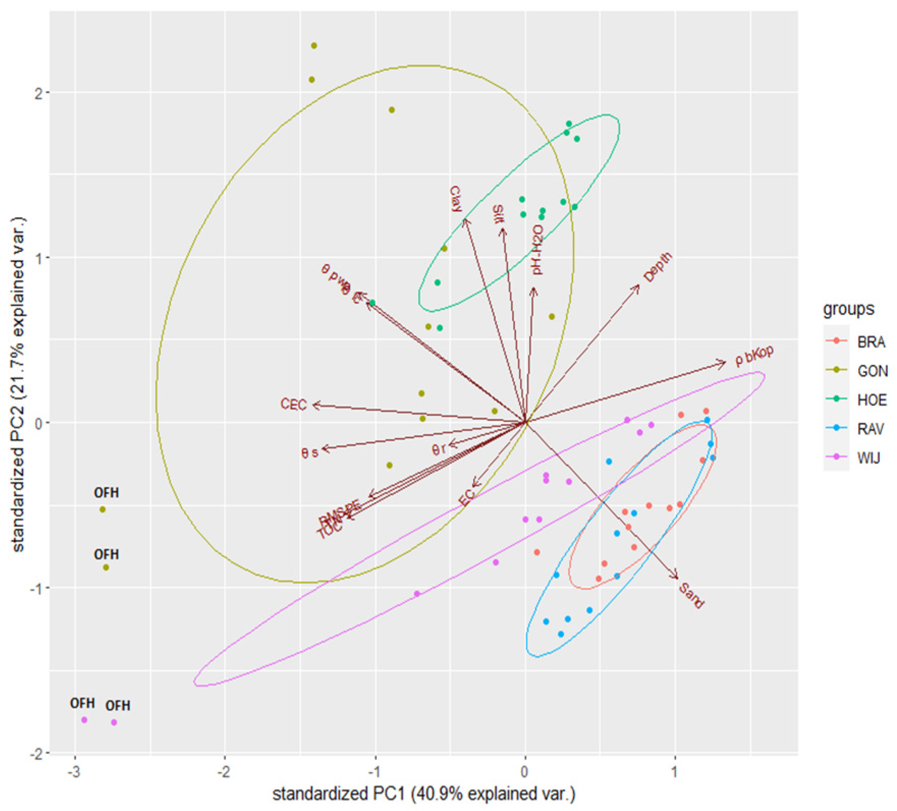
4.2. FDR Response to Soil Properties

It is well known that the FDR response is affected by soil bulk density, clay and organic matter content, voids and also salts (electrical conductivity). Therefore, we believe it is best that each sensor is calibrated in situ for the specific soil horizon it is located in, since the unique combination of all these factors in each horizon is hard to simulate in the lab, let alone their interactions.
Soil bulk density (ρb) is one of the most spatially variable soil properties, especially in the topsoil of forest soils [33]. Moreover, if ρb is not determined from the same sample as the mass basis water content, there will be an error in the calculation of θv [11] and this may seriously affect the quality of any calibration or validation dataset.
Bulk density in forest soils is strongly and inversely related with organic matter content, which is its best predictor. The more organic the soil, the lower ρb, the higher the meso- and macroporosity and the more water can be stored in the soil. In fine textured soils, such as clays, their volume will change as they dry, so their ρb may not be a constant and the relationship between FDR response and ρb may not be constant as well. Besides, if the soils shrink, this might change the contact of the rods with the soil which will affect measurement accuracy.
The response of the CS616 to changing water content has been shown to change for some soils when bulk density exceeds 1500 kg m−3, which is seldom the case for the studied soils. This response to changing water content is still well behaved, but the slope will decrease with increasing bulk density [20]. Most laboratory calibrations in small or larger containers try to mimic the average soil ρb of the field. Since ρb is strongly determining the RMSPE as we found in our study, lab conditions will presumably underestimate real intrinsic variation in field conditions and thus underestimate real RMSPE.
A big advantage of the CS616 is its larger measurement volume—about 3740 cm3 compared to other EM sensors mostly below 1000 cm3 [10]—which results in less spatial variability than probes with a smaller measurement volume [3]. We expect effects from ρb and other soil properties to be averaged over the 30 cm long rods.
The amount of organic matter and clay in a soil can alter the response of dielectric-dependent methods to changes in water content. This is apparent when mechanistic models are used to describe this measurement methodology, but less clear by using empirical calibration models [11]. Standard calibration coefficients are given for the CS616 for mineral soils with clay content less than 30% [20]. Consequently, higher clay contents require specific calibration but this calibration is also influenced by conductivity, compaction (ρb) and temperature. Therefore [10] suggested that manufacturers supply calibration relationships for a general group of mineral soils (covering a wide range of textures) and specifically for sandy and clayey soils. Udawatta et al. [15] suggested that future research should focus on the effects of clay mineralogy on FDR response.
We found that fitting calibration functions for topsoil layers and especially for OFH layers as part of the forest floor is quite complex and difficult. This is partly due to the high intrinsic heterogeneity of the organo-mineral topsoils in forests both for the organic matter content and the resulting ρb.
Since most studies on FDR are conducted in arable soils, we found no papers dealing with FDR measurements in forest floor layers. For TDR, Schaap et al. [34] developed an adequate linear calibration function for forest floor media. They report negligible effects of decomposition, residual water and temperature on the calibration parameters, but a strong effect of shrinkage of the organic material both influencing θv and TDR reflection times, which may cause errors up to 0.02 m3 m−3 if not accounted for. We expect the same effects with FDR instruments. More research of FDR performance in forest floors and organo-mineral soils is definitely needed.
It is clear from Table 10 and Figure A1 that standard functions are inadequate for predicting θv in forest floors but also in organo-mineral topsoils (Ah layers or M01). Problems start when taking the calibration samples for sensors located in forest floors of variable thickness (5–9 cm in our study) if the steel cylinders are already 5 cm in height. Impossible to avoid sampling of mineral soil material. Similarly, sampling M01 without collecting forest floor material is also tentative. In our study we applied a ρb threshold to discriminate real forest floor samples from those contaminated with mineral soil, but this is a surrogate solution. Anyway, it helped us to lower RMSPE from 0.22 to 0.05 m3 m−3 which is surprisingly similar to the RMSPE of 0.06 m3 m−3 found by [10] for organic layers, using the calibration function of [15]: θFDR = −0.283 + 0.0182PA + 0.0002PA2.
Vaz et al. [10] concluded that for the organic samples, FDR sensor outputs are in general lower than for mineral soils. This is expected due to the low ρb. and high porosity of organic materials. This statement is confirmed by the increasing slope in Figure 8b compared to all samples (including mineral).
Accurate sensor readings depend on the absence of air gaps between the CS616 rods and soil [13]. Their study showed that 50% of the sensed volume is concentrated in the first 6 mm around and between the rods. So, hence heterogeneity of materials or air gaps should be avoided. However, since forest soils are full of life, bioturbation may cause tunnels or gaps around sensor rods affecting the readings. In addition, cracking or shrinking processes in clayey soils, such as in GON, might have disturbed sensor readings.
Campbell Ltd. [20] indicates that soils exhibiting bulk electrical conductivity (BEC) > 500 µS cm–1 will require a specific calibration. All soils in this study have an EC value well below 500µS/cm (Table 1), so this was no issue in our study.
Metallic soil components such as ironstone, or sesquioxide rich Bs horizons may affect FDR sensor readings [11] but we found no studies confirming that. Similarly, large knowledge gaps exist for possible effects of soil biota (roots, mycorrhiza) affecting FDR measurements, since these are transporting water. What if roots align with or cross the rods of the CS616, which makes sense if these sensors are installed for decades. Kang et al. [35] studied plant root growth effects in horticultural substrates. They found that various root size indicators (root fresh weight, root dry weight, and root water content) all had a negative effect on the estimation of θv by FDR sensors and that this effect should be considered in research applications.
Several authors recommended considering soil temperature in the calibration process of the CS616, since they found that diurnal fluctuations in soil temperature influenced the sensor readings [3,4].
Varble et al. [4] suggested making sensor readings during periods that the soil temperature is similar (for example, every early in the morning). Our calibration dataset was compiled with observations just before or after noon, so a possible diurnal effect could not be observed in our study. However, the recalibrated functions are applied to diurnal sensor outputs and could therefore induce extra prediction error for data at night. Presumably this possible error will be greater in the topsoil than in the subsoil due to temperature damping with increasing depth.
We found that temperature correction applied in standard functions may significantly reduce bias, but had a limited effect on precision error. So, a possible bias may be introduced due to temperature effects and it is worthwhile to quantify its magnitude, preferably in the field. The manufacturer mentions possible changes in water content due to temperature effects of up to 0.005 m3 m–3 °C–1 in clayey soils. The magnitude of the temperature sensitivity changes with water content, so the temperature correction assumes that both the water content and temperature do not vary over the length of the probe’s rods [20]. With recalibration we found also that models including temperature correction were rarely supported (using AICs) as best models in the topsoil, but rather in (some) subsoil layers. This may suggest that there is a risk of overfitting the calibration function by including temperature correction given the low number of replicates.
A similar conclusion was drawn by [13]. They found that temperature compensation was not satisfactory for most of the layers they calibrated. It may be necessary for soils with high EC (>500 µS/cm) or electrically lossy clays (large surface area and CEC).

4.3. Spatio-Temporal Variation of Soil Water Content

We observed a quite high variability among the three gravimetric reference measurements in each layer (Figures S1–S5), especially in the topsoil. A more stable calibration value would have been obtained by 4 reference measurements around each sensor or 12 measurements per layer. The number of calibration samples per layer is ideally derived from autocorrelation lengths based on spatio-temporal variogram studies of soil moisture measurements in forest soils. However, Huisman et al. [36] state that determination of correlation length from experimental variograms is highly uncertain even in the case of 100+ soil moisture measurements. Instead, they recommend ground penetrating radar measurements to assess spatial water content variation over time, but this technique might have its limitations in forest soils due to the presence of a forest floor and permanent root systems. Vereecken et al. [37] pointed out that many studies have shown that the correlation scale itself varies as a function of soil moisture content and increases as the soil is drying. So, there is a temporal dimension as well to account for. All of these studies indicate that the temporal variation of the correlation length is controlled by an interplay of several forcings, including throughfall, evapotranspiration and structural elements such as topography and soil properties and deterministic modelling using all these factors is difficult. From the three profiles studied per plot (Figure A1, Figure A2, Figure A3, Figure A4 and Figure A5 and Figures S1–S5), we found indications for inhomogeneous soil properties affecting soil moisture measurements and the principal components analysis confirmed that ρb, TOC and clay content are important controls. However, intrinsic heterogeneity due to micro-topography, drainage ditches, location of trees and ground vegetation patches could also play a role affecting soil moisture measurements. A dedicated multi-annual soil moisture monitoring on a highly instrumented site on one of the most variable plots (e.g., GON) would help to better understand how spatio-temporal variation of soil water content can be explained.

5. Conclusions

On all sites, in situ recalibration removed the bias of standard functions up to 0.16 m3 m−3 in topsoils and reduced the overall prediction error by a factor of 1.8 to 2.8. Standard functions performed very poorly in organic and organo-mineral topsoil layers and clayey substrates. Definitely, recalibration is required for each location where an FDR sensor is installed and new layer-specific empirical calibration functions have to be developed for each site in order to meet the data quality objectives (bias less than 0.01 m3 m−3 and RMSPE < 0.03 m3 m−3).
However, average single FDR sensor accuracy for the studied forest soils is 0.043 m3 m−3 so for most layers multiple sensors are required to predict average θv with an accuracy better than 0.03 m3 m−3 at the plot scale. Operators should be aware of the level of effective field accuracy of their sensors.
Prediction bias is strongly related with clay content and soil depth and therefore there is a need for depth specific empirical calibration functions or mechanistic functions that incorporate clay content and depth variables. Precision error is most positively related to carbon content (organic matter) and negatively with soil bulk density. Especially organo-mineral topsoil layers showing high ρb variation are hard to calibrate in situ due to imprecise field measurements. The current number of sensors at GON is too low to reduce the total measurement error and this might thwart future application of water balance models for environmental modeling purposes.
For most sites, more than 19 monthly calibrations are required to lower the bias consistently below 0.01 m3 m−3, which is in fact a 2 drying and 1 rewetting phase if calibration started when soils are near field capacity. We recommend intensifying the calibration sampling during the growing season, for instance by two-weekly sampling instead of monthly for a better spread of calibration points between field capacity and permanent wilting point.
Finally, we found that two to three FDR sensors per layer for the Flemish ICP Forests Level II study plots are adequate to reach an acceptable measurement accuracy in the homogeneous sand and silt loam sites, but up to 10 to 16 sensors may be required in heterogeneous topsoil or clayey subsoil layers of the other sites to account for their high intrinsic variability, otherwise hydrological modeling will be tentative.
Future research should focus on development of dedicated calibration functions for forest floors and other organic layers followed by an adequate in situ validation.

Supplementary Materials

The following Supplementary data are available online at https://www.mdpi.com/article/10.3390/app112411620/s1. Figures S1–S5—Layer specific relationships between reference gravimetric water content and FDR sensor measurements for each site; Tables S1–S5 with Coefficients and predictive quality of standard calibration functions for all profiles and depths of the 5 plots; 5 calibration datasets (excel) with corresponding recalibrated FDR measurements: WIJ.calibDB.xlsx, RAV.calibDB.xlsx, BRA.calibDB.xlsx, GON.calibDB.xlsx and HOE.calibDB.xlsx.

Author Contributions

This study was mainly conducted by B.D.V., but FDR sensor data was collected, validated and stored by A.V. and N.C. (physico-chemical soil data). Review and editing by J.N., A.V., and N.C. All authors have read and agreed to the published version of the manuscript.

Funding

This research received no external funding.

Institutional Review Board Statement

Not applicable.

Informed Consent Statement

Not applicable.

Data Availability Statement

Survey and monitoring data (soil, meteo, deposition) of the studied LII plots are available from the ICP Forests database residing at the Programme Co-ordinating Centre (PCC) of ICP Forests in Eberswalde, Germany. Data requests and Intellectual Property Publication Policy can be found at http://icp-forests.net/page/data-requests (accessed on 10 August 2021).

Acknowledgments

We especially thank Frederic Vermeiren and Eddy Smesman for the installation and initial calibration/testing of the FDR sensors at the five sites and starting up the monitoring in 2010. Technical support for this study by Koen Willems, Koen Vervaet and Mathieu Pieters for the monthly field sampling and measurements of ρb and θv (reference dataset), and by Yvan De Bodt for FDR data logger read-outs and data assembly is greatly appreciated and acknowledged. We also thank the Flemish Agency for Forest and Nature (ANB) for access, use and maintaining the forest sites for long term monitoring and research. Last but not least we want to thank three anonymous reviewers for their constructive comments resulting in an improvement of this manuscript.

Conflicts of Interest

The authors declare no conflict of interest.

Appendix A

Table A1. Stand and site characteristics of the 5 Level II plots.
SiteWIJRAVBRAGONHOE
ICP Forests LII plot code 12_112_142_152_162_21
LocationWijnendaleRavelsBrasschaatGontrodeHoeilaart
Latitude [DD]51.0694651.4030651.3076250.9750150.74722
Longitude [DD]3.036125.056944.519823.804334.41472
Altitude [m asl]31351426129
MAT [°C]1110.410.810.610.7
MAP [mm]867887882786854
TypeDeciduous broadleavedEvergreen
coniferous
Evergreen
coniferous
Deciduous
broadleaved
Deciduous
broadleaved
EFTC 26.Beech forest14.Introduced tree species2.Nemoral coniferous forest5.Mesophytic deciduous forest6.Beech forest
Dom. tree speciesFagus sylvaticaPinus nigraPinus sylvestris; Betula pendulaQuercus robur;
Fagus sylvatica
Fagus sylvatica
Age [yr]869192103112
Top height 3 [m]30.5727.9622.3631.0137.18
Basal area 4 [m2]30.9742.5628.5336.3933.30
Stem density 5 [n/ha]152404576548224
Humus system 6MorMorMorModerModer
Reference Soil Group 7UmbrisolArenosolArenosolPlanosolRetisol
Soil qualifiers 7Endogleyic, Folic, Endoaric, EndorapticHyperdystric, Albic, Endogleyic, Folic, HumicHyperdystric, Albic, Brunic, Gleyic, Aric, RapticEutric, Luvic, Folic, Clayic, Siltic, Ochric, EndorapticHyperdystric, Glossic, Fragic, Abruptic, Cutanic, Differentic, Pantosiltic, Profondic
Parent MaterialEolian sandsEolian sandsEolian sandsLoamy loess on Tertiary clayLoamy loess
1 Plot code is concatenation of Country code_Plot number, 2 European Forest Type Category [24], 3 Top height is the average of all dominant trees with height > 19 m during winter 2019–2020, 4 Basal area is sum of all trees with diameter > 5 cm (winter 2019–2020), 5 Stem density is number of all trees with diameter > 5 cm (winter 2019–2020), 6 according to [25], 7 according to [23].
Table A2. FDR sensor depth (cm) relative to the top of the mineral horizon. Negative depths are in the forest floor. Center of Kopecky cylinders for reference sampling are situated at the same depth.
WIJ RAV BRA GON HOE
LayerABCABCABCABCABC
OFH −2−4 −3−4
M012 112.53.5074 554
M1212.511816131415162517719192015
M24363128303129353640372035394542
M48576159606162736660585558626660
Table A3. Summary statistics of calibration dataset by site and soil layer.
Depth Period Average (PA, µs)Soil Temperature (ST, °C) 1Bulk Density (ρbKop, kg m−3)Gravimetric SWC (Ɵm, g kg−1)Volumetric SWC (Ɵv, m3 m−3)
SiteSeq.LayernMeanCI95 MeanRangeMeanCI95 MeanRangeMeanCI95 MeanRangeMeanCI95 MeanRangeMeanCI95 MeanRange
WIJ1OFH4727.8[26.9, 28.7]20.5–32.511.5[9.2, 15.2]5.5–25.0559[498, 616]190–8401343[1139, 1609]493–34760.59[0.57, 0.61]0.41–0.73
1M012828.7[27.6, 29.5]20.3–32.112.5[10.2, 16.2]6.4–24.21066[1010, 1122]870–1320404[367, 442]208–5930.42[0.39, 0.44]0.27–0.53
2M127524.2[23.8, 24.6]19.7–26.410.6[9.5, 11.8]6.2–15.41335[1290, 1358]420–1530221[200, 301]117–15920.28[0.27, 0.30]0.14–0.67
3M247524.2[23.6, 24.9]18.4–30.010.5[9.6, 11.6]6.7–14.91317[1297, 1335]1110–1500208[198, 218]117–3350.27[0.26, 0.29]0.15–0.41
4M487524.6[23.9, 25.3]18.4–28.710.4[9.5, 11.4]7–14.51441[1418, 1461]1130–1620195[182, 209]76.4–3790.28[0.26, 0.29]0.11–0.46
RAV1OFH221.6-18.6–24.615.8-15.8–15.8765-690–840470-260–6800.35-0.23–0.47
1M017322.7[22.1, 23.4]17.8–29.410.2[8.8, 11.6]4.6–16.71434[1395, 1467]990–1660179[165, 196]53.2–4090.25[0.23, 0.27]0.07–0.43
2M127523.5[23.1, 24.0]18.4–26.310.4[9.2, 11.6]5.4–15.81461[1434, 1485]1150–1660136[125, 148]43–2620.2[0.18, 0.21]0.06–0.34
3M247521.7[21.3, 22.1]17.7–24.810.5[9.4, 11.7]5.8–15.61399[1376, 1422]1190–1670143[133, 154]48–2980.2[0.18, 0.21]0.06–0.36
4M487519.7[19.5, 20.1]17.9–26.410.4[9.4, 11.4]6.4–14.51602[1582, 1617]1310–176074.3[68.4, 82.6]27.9–2130.12[0.11, 0.13]0.05–0.28
BRA1M017521.7[21.3, 22.2]17.4–26.210.7[9.1, 12.4]4.1–17.71378[1337, 1407]640–1570154[140, 177]49.1–6030.2[0.19, 0.22]0.07–0.39
2M127521.2[20.7, 21.6]17.0–25.510.7[9.3, 12.2]4.8–16.31440[1416, 1460]1140–1590130[120, 142]38.4–3010.19[0.17, 0.20]0.05–0.38
3M247520.2[19.9, 20.4]17.2–22.410.9[9.7, 12.2]5.7–16.01494[1476, 1513]1220–1700115[106, 124]38.5–2280.17[0.16, 0.19]0.06–0.33
4M487522.9[22.5, 23.3]18.2–26.610.7[9.6, 11.8]6.4–15.31549[1532, 1564]1280–1700121[112, 129]48.8–2010.19[0.17, 0.20]0.08–0.30
GON1OFH5030.2[29.4, 31.0]23.6–34.110.5[8.7, 12.3]4.1–16.1509[450, 570]200–8301495[1255, 1787]370–34490.58[0.54, 0.61]0.22–0.78
1M012530[29.1, 30.9]24.7–33.99.8[7.7, 12.1]5.7–15.61031[986, 1084]870–1300469[431, 523]295–8240.47[0.45, 0.52]0.36–0.78
2M127528[27.5, 28.5]22.2–31.110.3[9.1, 11.6]4.9–15.71095[1050, 1141]550–1440400[366, 440]158–10360.41[0.39, 0.43]0.18–0.59
3M247531.1[29.8, 32.2]20.2–38.310.2[9.0, 11.4]5.3–15.21221[1177, 1261]530–1580325[300, 356]115–8040.38[0.36, 0.40]0.14–0.59
4M487538.6[37.9, 39.2]31.7–41.910.1[9.1, 11.2]5.7–14.71193[1149, 1241]720–1740394[364, 423]151–6830.45[0.42, 0.47]0.22–0.62
HOE1OFH229.6-28.9–30.24.8--775-700–850818-674–9620.62-0.57–0.68
1M017627.7[27.1, 28.3]21.7–31.09.9[8.5, 11.3]4.5–15.41239[1209, 1268]900–1480364[344, 386]182–6600.44[0.42, 0.46]0.25–0.59
2M127827.1[26.5, 27.6]21.6–29.69.6[8.4, 11.0]4.6–15.11430[1410, 1451]1220–1700255[242, 267]127–3720.36[0.35, 0.38]0.16–0.48
3M247827.9[27.5, 28.2]23.4–29.49.7[8.5, 11.0]5.0–14.91539[1515, 1560]1290–1770222[212, 232]133–3650.34[0.33, 0.35]0.18–0.47
4M487829.2[29.0, 29.3]27.0–30.59.5[8.4, 10.6]5.2–14.21571[1554, 1587]1400–1710218[212, 224]161–2910.34[0.33, 0.35]0.23–0.43
1 Soil temperature is measured in Profile A only.
Table A4. AICc based selection of best and second best recalibrated model types for each profile and layer with AICc weights (AICsWt) and evidence ratios (ER). The ER indicates how many times more parsimonious the best model is over the second best model.
SiteProfileLayerBest ModelAICcWt2nd Best ModelAICcWtER
WIJAM01LM0.506LMTC0.2502.03
M12LMTC0.496LM0.3051.63
M24LMTC0.529LM0.2642.00
M48LM0.323LMTC0.2421.33
BOFHQM0.422LM0.2491.70
M12QMTC0.504QM0.1972.56
M24LM0.392LMTC0.2921.34
M48LMTC0.440LM0.3651.21
COFHLM0.400LMTC0.3841.04
M12LM0.508LMTC0.2821.80
M24QMTC0.483QM0.4511.07
M48LM0.428LMTC0.3521.21
RAVAM01LM0.407LMTC0.3911.04
M12LMTC0.505LM0.2581.96
M24LM0.406LMTC0.3991.02
M48LMTC0.365LM0.2871.27
BM01LM0.472LMTC0.3201.47
M12LM0.281LMTC0.2771.01
M24LM0.392LMTC0.2921.34
M48LM0.520QM0.2262.30
CM01LMTC0.432LM0.3371.28
M12QM0.949QMTC0.04222.8
M24LM0.431LMTC0.2171.98
M48QM0.645QMTC0.3142.05
BRAAM01LM0.463LMTC0.3291.41
M12LM0.420LMTC0.3701.14
M24QM0.308LMTC0.2511.23
M48QM0.498LM0.2402.07
BM01LM0.449LMTC0.2591.73
M12LM0.419LMTC0.3191.31
M24LM0.427LMTC0.3291.30
M48LMTC0.413LM0.2441.69
CM01LM0.412LMTC0.2961.39
M12QMTC0.630LMTC0.1693.73
M24LMTC0.549LM0.2552.16
M48LM0.390LMTC0.3411.14
GONAM01LM0.712QM0.1793.97
M12QM0.314LM0.2891.09
M24LMTC0.427LM0.3501.22
M48LMTC0.498LM0.2501.99
BOFHLM0.667QM0.1693.95
M12QMTC0.821LMTC0.0928.90
M24LMTC0.472LM0.3051.55
M48LM0.343LMTC0.3361.02
COFHLM0.574LMTC0.2172.65
M12QMTC0.558LM0.2402.32
M24LM0.657QM0.2682.45
M48QMTC0.488LM0.2262.16
HOEAM01LM0.552LMTC0.2152.57
M12QM0.468LM0.3081.52
M24LMTC0.690QMTC0.1813.81
M48LMTC0.395LM0.3681.07
BM01QM0.374LM0.3061.23
M12LM0.532QM0.2961.80
M24LMTC0.612QMTC0.2282.68
M48LM0.389LMTC0.2641.47
CM01LM0.462LMTC0.2871.61
M12LM0.530QM0.3041.74
M24LM0.630QM0.1703.70
M48LM0.720QM0.1764.08
Table A5. Finally selected recalibrated functions for all sites and layers with their prediction quality indices.
CoefficientsPrediction Quality
SiteProfileLayerModelC0C1C2R2adjRMSPEdr
WIJAM01LM−0.6063120.036363-0.1020.11650.547
M12LMTC−0.2426660.020704-0.7870.02130.794
M24LMTC−0.1365950.016481-0.8220.02820.792
M48LM−0.3617670.025925-0.8590.03170.833
BOFHLM0.399620.008767-0.2760.04170.562
M12LMTC−0.443170.028264-0.3040.07630.596
M24LM−0.339850.024922-0.7530.02780.751
M48LMTC−0.260830.020252-0.7920.03070.78
COFHLM0.399620.008767-0.2760.04170.562
M12LM−0.21880.021074-0.6740.02170.715
M24QMTC−0.97550.091207−0.00160.7310.02780.748
M48LM−0.109140.016292-0.7930.03290.787
RAVAM01LM0.1288510.004916-0.0120.0620.504
M12LMTC−0.308480.02074-0.470.04180.659
M24LM−0.310940.023671-0.5270.03370.654
M48LMTC−0.409850.025594-0.7180.01150.737
BM01LM−0.229220.023997-0.4180.05960.592
M12LM−0.037780.010414-0.1260.06060.519
M24LM−0.131180.016274-0.180.05330.582
M48LM−0.465010.029232-0.6930.0150.749
CM01LMTC−0.085910.012619-0.2710.06730.567
M12LM−0.542360.030826-0.6060.04620.686
M24LM−0.464450.028796-0.6130.03790.723
M48QM−1.8119080.159353−0.0030510.8270.01880.786
BRAAM01LM−0.461950.029329-0.5720.05310.71
M12LM−0.46550.032457-0.5690.04190.674
M24QM3.513639−0.391080.011130.630.0320.697
M48QM2.004305−0.184410.004450.7420.0240.749
BM01LM−0.375210.026302-0.450.05190.638
M12LM−0.463840.032053-0.5770.03820.688
M24LM−0.455030.030181-0.6340.02910.707
M48LMTC−0.26540.020287-0.6210.02970.665
CM01LM−0.402770.029549-0.4680.05110.664
M12QMTC2.685401−0.249470.006050.5910.04380.659
M24LMTC−0.678440.042803-0.5640.04460.649
M48LM−0.279220.021949-0.5280.03570.627
GONAM01LM−0.707510.043-0.5160.06770.618
M12QM3.422366−0.279490.0061710.6970.04610.723
M24LMTC−0.285580.02309-0.8030.04090.814
M48LMTC0.0644550.008269-0.2390.07550.545
BOFHLM−0.4502620.033966-0.7160.05910.749
M12LMTC−0.3097090.02574-0.5090.05880.625
M24LMTC−0.421310.022229-0.4560.05890.616
M48LM0.1670120.008683-0.0570.06180.513
COFHLM−0.4502620.033966-0.7160.05910.749
M12LM−0.3895480.027291-0.1240.0750.513
M24LM−0.685470.032331-0.2660.04680.558
M48LM0.224040.004552-0.0030.09980.495
HOEAM01LM−0.327410.026886-0.5760.04420.685
M12QM−2.73240.202518−0.003240.9160.02010.872
M24LMTC−0.957990.043073-0.730.02690.77
M48LMTC−0.645290.032059-0.7050.02270.74
BM01QM−1.561270.128421−0.002040.8350.02870.793
M12LM−0.461190.030068-0.9550.0190.91
M24LMTC−0.637090.032494-0.7970.02880.779
M48LM−0.886830.0411-0.660.02440.718
CM01LM0.0229780.016508-0.3740.05470.602
M12LM−0.297280.024898-0.8650.02450.823
M24LM−0.359070.026401-0.670.03610.686
M48LM−0.833250.04117-0.7490.02180.74

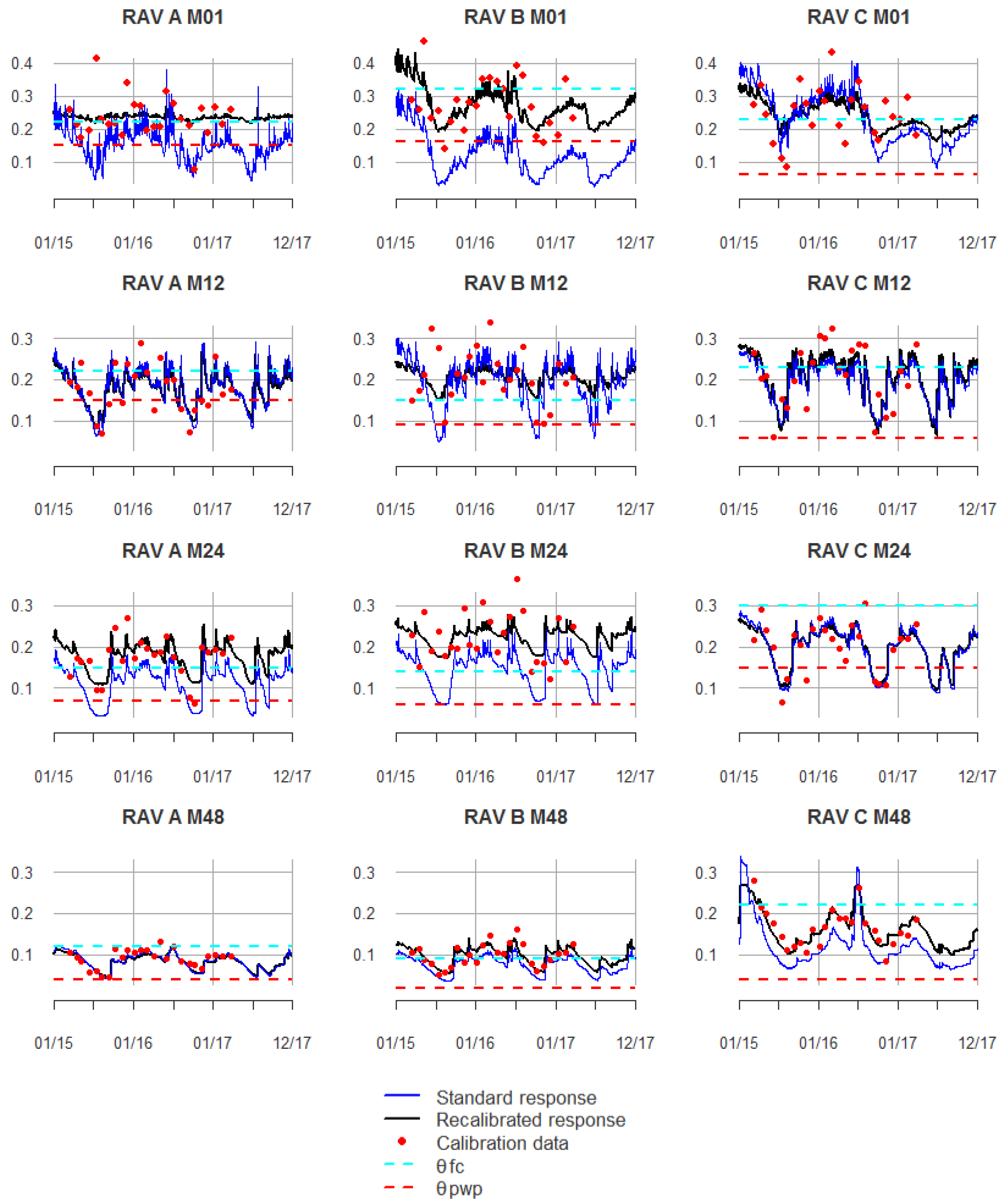
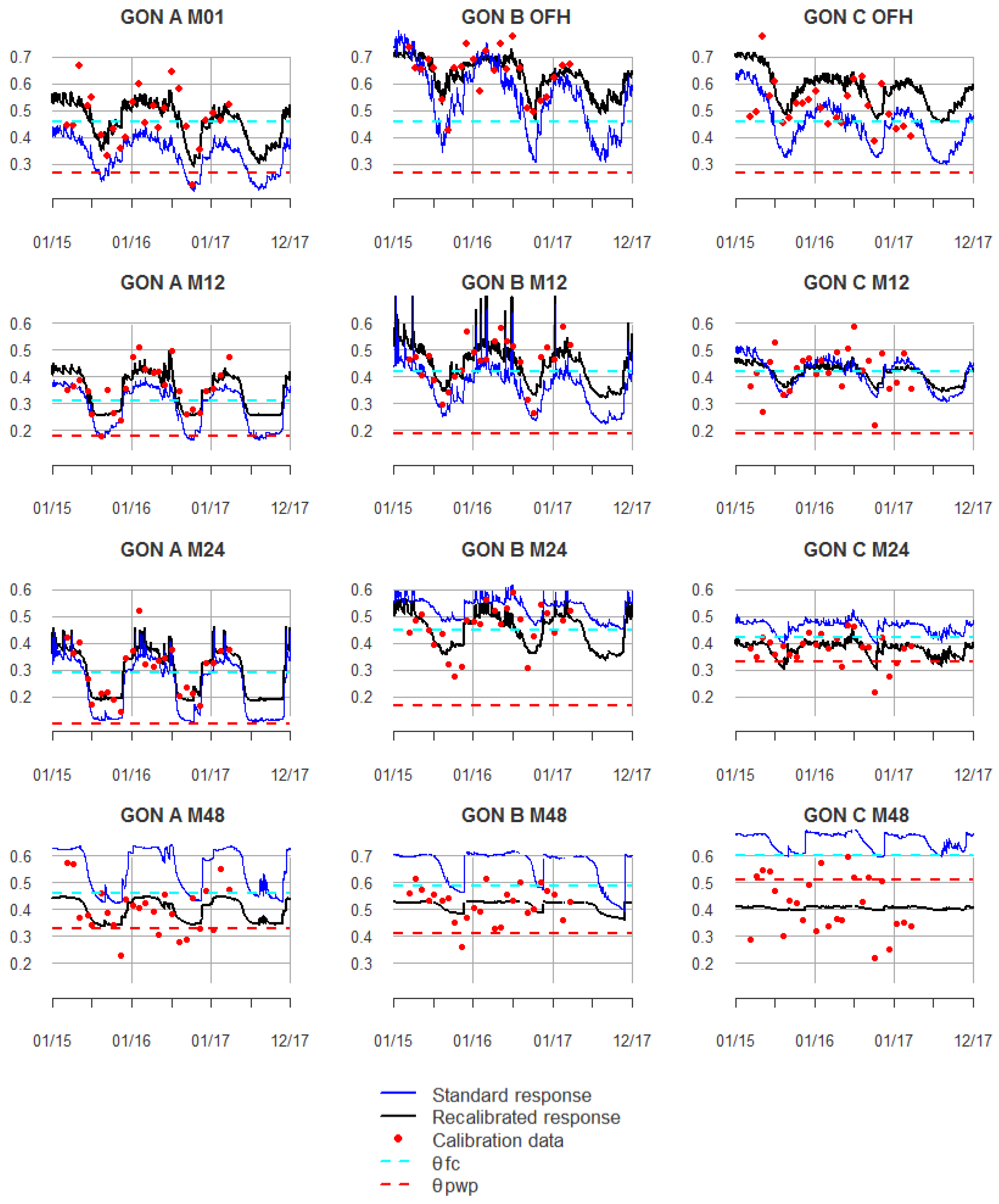
Appendix B. Standard and Recalibrated Soil Water Series

Figure A1. Soil water content (m3 m−3) according to standard and recalibrated functions for each profile and layer of the WIJ plot with indication of field capacity and permanent wilting point for mineral soils (dashed lines).
Applsci 11 11620 g0a1
Figure A2. Soil water content (m3 m−3) according to standard and recalibrated functions for each profile and layer of the RAV plot with indication of field capacity and permanent wilting point for mineral soils (dashed lines).
Applsci 11 11620 g0a2
Figure A3. Soil water content (m3 m−3) according to standard and recalibrated functions for each profile and layer of the BRA plot with indication of field capacity and permanent wilting point for mineral soils (dashed lines).
Applsci 11 11620 g0a3
Figure A4. Soil water content (m3 m−3) according to standard and recalibrated functions for each profile and layer of the GON plot with indication of field capacity and permanent wilting point for mineral soils (dashed lines).
Applsci 11 11620 g0a4
Figure A5. Soil water content (m3 m−3) according to standard and recalibrated functions for each profile and layer of the HOE plot with indication of field capacity and permanent wilting point for mineral soils (dashed lines).
Applsci 11 11620 g0a5

References

  1. Dong, Y.; Miller, S.; Kelley, L. Performance Evaluation of Soil Moisture Sensors in Coarse-and Fine-Textured Michigan Agricultural Soils. Agriculture 2020, 10, 598. [Google Scholar] [CrossRef]
  2. Kelleners, T.; Seyfried, M.; Blonquist, J., Jr.; Bilskie, J.; Chandler, D. Improved interpretation of water content reflectometer measurements in soils. Soil Sci. Soc. Am. J. 2005, 69, 1684–1690. [Google Scholar] [CrossRef]
  3. Logsdon, S. CS616 calibration: Field versus laboratory. Soil Sci. Soc. Am. J. 2009, 73, 1–6. [Google Scholar] [CrossRef]
  4. Varble, J.L.; Chávez, J. Performance evaluation and calibration of soil water content and potential sensors for agricultural soils in eastern Colorado. Agric. Water Manag. 2011, 101, 93–106. [Google Scholar] [CrossRef]
  5. Mittelbach, H.; Lehner, I.; Seneviratne, S.I. Comparison of four soil moisture sensor types under field conditions in Switzerland. J. Hydrol. 2012, 430, 39–49. [Google Scholar] [CrossRef]
  6. Bogena, H.R.; Huisman, J.A.; Schilling, B.; Weuthen, A.; Vereecken, H. Effective calibration of low-cost soil water content sensors. Sensors 2017, 17, 208. [Google Scholar] [CrossRef] [PubMed] [Green Version]
  7. Veldkamp, E.; O’Brien, J.J. Calibration of a frequency domain reflectometry sensor for humid tropical soils of volcanic origin. Soil Sci. Soc. Am. J. 2000, 64, 1549–1553. [Google Scholar] [CrossRef]
  8. Blonquist, J., Jr.; Jones, S.B.; Robinson, D.A. Standardizing characterization of electromagnetic water content sensors: Part 2. Evaluation of seven sensing systems. Vadose Zone J. 2005, 4, 1059–1069. [Google Scholar] [CrossRef]
  9. Czarnomski, N.M.; Moore, G.W.; Pypker, T.G.; Licata, J.; Bond, B.J. Precision and accuracy of three alternative instruments for measuring soil water content in two forest soils of the Pacific Northwest. Can. J. For. Res. 2005, 35, 1867–1876. [Google Scholar] [CrossRef] [Green Version]
  10. Vaz, C.M.; Jones, S.; Meding, M.; Tuller, M. Evaluation of standard calibration functions for eight electromagnetic soil moisture sensors. Vadose Zone J. 2013, 12, 1–16. [Google Scholar] [CrossRef]
  11. Hignett, C.; Evett, S.R.; Heng, L.K.; Moutonnet, P.; Nguyen, M.L. Field Estimation of Soil Water Content: A Practical Guide to Methods, Instrumentation, and Sensor Technology; IAEA: Vienna, Austria, 2008. [Google Scholar]
  12. De Vos, B. Capability of PlantCare Mini-Logger Technology for Monitoring of Soil Water Content and Temperature in Forest Soils; INBO: Geraardsbergen, Belgium, 2015; p. 82. [Google Scholar]
  13. Ruelle, P.; Laurent, J.P. CS616 (CS615) Water Content Reflectometer. In Field Estimation of Soil Water Content. A Practical Guide to Methods Instrumentation and Sensor Technology; Hignett, C., Evett, S., Eds.; International Atomic Energy Agency: Vienna, Austria, 2008; pp. 101–110. [Google Scholar]
  14. Rüdiger, C.; Western, A.W.; Walker, J.P.; Smith, A.B.; Kalma, J.D.; Willgoose, G.R. Towards a general equation for frequency domain reflectometers. J. Hydrol. 2010, 383, 319–329. [Google Scholar] [CrossRef]
  15. Udawatta, R.P.; Anderson, S.H.; Motavalli, P.P.; Garrett, H.E. Calibration of a water content reflectometer and soil water dynamics for an agroforestry practice. Agrofor. Syst. 2011, 82, 61–75. [Google Scholar] [CrossRef]
  16. Topp, G.C.; Davis, J.; Annan, A.P. Electromagnetic determination of soil water content: Measurements in coaxial transmission lines. Water Resour. Res. 1980, 16, 574–582. [Google Scholar] [CrossRef] [Green Version]
  17. Jackisch, C.; Germer, K.; Graeff, T.; Andrä, I.; Schulz, K.; Schiedung, M.; Haller-Jans, J.; Schneider, J.; Jaquemotte, J.; Helmer, P. Soil moisture and matric potential–an open field comparison of sensor systems. Earth Syst. Sci. Data 2020, 12, 683–697. [Google Scholar] [CrossRef] [Green Version]
  18. Ziche, D.; Riek, W.; Russ, A.; Hentschel, R.; Martin, J. Water Budgets of Managed Forests in Northeast Germany under Climate Change—Results from a Model Study on Forest Monitoring Sites. Appl. Sci. 2021, 11, 2403. [Google Scholar] [CrossRef]
  19. Raspe, S.; Fleck, S.; Beuker, E.; Preuhsler, T.; Bastrup-Birk, A. Meteorological Measurements. In Manual on Methods and Criteria for Harmonized Sampling, Assessment, Monitoring and Analysis of the Effects of Air Pollution on Forests; UNECE ICP Forests, Programme Coordinating Centre, Ed.; Thünen Institute of Forest Ecosystems: Eberswalde, Germany, 2008; 18p, Available online: http://www.icp-forests.org/manual.htm (accessed on 10 August 2021).
  20. Campbell Scientific. CS616 and CS625 Water Content Reflectometers, Instruction Manual 2020. Revision: 05/20. Available online: https://s.campbellsci.com/documents/eu/manuals/cs616_625%20-%20467.pdf (accessed on 13 January 2021).
  21. USDA. Keys to Soil Taxonomy, 12th ed.; Soil Survey Staff: Washington, DC, USA, 2014; 372p.
  22. Cockx, K.; Van Meirvenne, M.; De Vos, B. Using the EM38DD Soil Sensor to Delineate Clay Lenses in a Sandy Forest Soil. Soil Soc. Am. J. 2007, 71, 1314–1322. [Google Scholar] [CrossRef]
  23. IUSS Working Group WRB. World Reference Base for Soil Resources 2014, Update 2015 International Soil Classification System for Naming Soils and Creating Legends for Soil Maps; FAO: Rome, Italy, 2015. [Google Scholar]
  24. Giannetti, F.; Barbati, A.; Davide Mancini, L.; Bastrup-Birk, A.; Canullo, R.; Nocentini, S.; Chirici, G. European forest types: Toward an automated classification. Ann. For. Sci. 2018, 75, 6. [Google Scholar] [CrossRef] [Green Version]
  25. Zanella, A.; Ponge, J.-F.; Jabiol, B.; Sartori, G.; Kolb, E.; Le Bayon, R.-C.; Gobat, J.-M.; Aubert, M.; De Waal, R.; Van Delft, B. Humusica 1, article 5: Terrestrial humus systems and forms—Keys of classification of humus systems and forms. Appl. Soil Ecol. 2018, 122, 75–86. [Google Scholar] [CrossRef]
  26. Fleck, S.; Cools, N.; De Vos, B.; Meesenburg, H.; Fischer, R. The Level II aggregated forest soil condition database links soil physicochemical and hydraulic properties with long-term observations of forest condition in Europe. Ann. For. Sci. 2016, 73, 945–957. [Google Scholar] [CrossRef] [Green Version]
  27. Cools, N.; De Vos, B. Part X: Sampling and Analysis of Soil. In Manual on Methods and Criteria for Harmonized Sampling, Assessment Monitoring and Analysis of the Effects of Air Pollution on Forests; UNECE ICP Forests Programme Coordinating Centre, Ed.; Thünen Institute of Forest Ecosystems: Eberswalde, Germany, 2020; 115p, Available online: http://www.icp-forests.org/Manual.htm (accessed on 16 May 2021).
  28. Van Genuchten, M.T. A closed-form equation for predicting the hydraulic conductivity of unsaturated soils. Soil Sci. Soc. Am. J. 1980, 44, 892–898. [Google Scholar] [CrossRef] [Green Version]
  29. De Vos, B.; Cools, N.; Ilvesniemi, H.; Vesterdal, L.; Vanguelova, E.; Carnicelli, S. Benchmark values for forest soil carbon stocks in Europe: Results from a large scale forest soil survey. Geoderma 2015, 251–252, 33–46. [Google Scholar] [CrossRef]
  30. R Core Team. R: A Language and Environment for Statistical Computing; R Foundation for Statistical Computing: Vienna, Austria. Available online: http://www.R-project.org/ (accessed on 10 August 2021).
  31. Mazerolle, M.J.; AICcmodavg: Model Selection and Multimodel Inference Based on (Q)AIC(c). R Package Version 2.3-1. Available online: https://cran.r-project.org/package=AICcmodavg (accessed on 10 August 2021).
  32. Willmott, C.J.; Robeson, S.M.; Matsuura, K. A refined index of model performance. Int. J. Climatol. 2012, 32, 2088–2094. [Google Scholar] [CrossRef]
  33. De Vos, B.; Van Meirvenne, M.; Quataert, P.; Deckers, J.; Muys, B. Predictive quality of Pedotransfer functions for estimating bulk density of forest soils. Soil Sci. Soc. Am. J. 2005, 69, 500–510. [Google Scholar] [CrossRef]
  34. Schaap, M.; De Lange, L.; Heimovaara, T. TDR calibration of organic forest floor media. Soil Technol. 1997, 11, 205–217. [Google Scholar] [CrossRef]
  35. Kang, S.; van Iersel, M.W.; Kim, J. Plant root growth affects FDR soil moisture sensor calibration. Sci. Hortic. 2019, 252, 208–211. [Google Scholar] [CrossRef]
  36. Huisman, J.; Snepvangers, J.; Bouten, W.; Heuvelink, G. Monitoring temporal development of spatial soil water content variation: Comparison of ground penetrating radar and time domain reflectometry. Vadose Zone J. 2003, 2, 519–529. [Google Scholar] [CrossRef]
  37. Vereecken, H.; Huisman, J.; Pachepsky, Y.; Montzka, C.; Van Der Kruk, J.; Bogena, H.; Weihermüller, L.; Herbst, M.; Martinez, G.; Vanderborght, J. On the spatio-temporal dynamics of soil moisture at the field scale. J. Hydrol. 2014, 516, 76–96. [Google Scholar] [CrossRef]
Figure 1. FDR installation, spatial sensor configuration and calibration sampling scheme. Profile pit A of BRA with installed FDR sensors (April 2010) according to four depth intervals; setup of FDR sensors in three pits (A, B, C) and temperature probes in pit A only; scheme indicating monthly sampling locations for calibration measurements 2 m north of each pit. Clockwise sampling at inner ring locations (Year 1, red) and outer ring (Year 2, green). At each location undisturbed samples were taken at the 4 depths.
Applsci 11 11620 g001
Figure 2. Example of (re)calibration of FDR response functions. (a) Measured values with response curve of standard function and recalibrated function for plot HOE, profile B and layer M12; (b) time series of predicted ƟFDR by standard function and by recalibrated function with indication of 26 monthly calibration points. Ticks on the X axis indicate months, vertical gridlines indicate years. Green, cyan, and red horizontal lines indicate respectively saturated water content, field capacity and permanent wilting point (Table 2).
Applsci 11 11620 g002
Figure 3. Predictive quality of standard linear and quadratic models for all plots, profiles and depth layers. Negative bias indicates underestimation of real soil water content. Red dashed lines show the allowable error threshold, black dotted line provides mean total prediction error (RMSPE).
Applsci 11 11620 g003
Figure 4. Overall prediction error of best performing standard function and best calibrated function for all plots, profiles and depth layers. The difference indicates the calibration gain. Red dashed lines show the allowable error threshold set at 0.03 m3 m−3. Scales are identical to illustrate differences among sites.
Applsci 11 11620 g004
Figure 5. Replacing (a) a non-monotonically increasing function with (b) a monotonic function for layer M12 in the GON C profile. Note that in (a) Output period is temperature corrected while in (b) it is not.
Applsci 11 11620 g005
Figure 6. Principal component analysis of the bias (MPE) of the standard LM and explaining soil variables. The observations are grouped by layers and indicated by color and ellipses.
Applsci 11 11620 g006
Figure 7. Principal component analysis of calibrated functions by layers (dots) and soil properties as vectors, grouped by plot.
Applsci 11 11620 g007
Figure 8. Scatterplots of topsoil calibration data relating sensor output to observed volumetric water content (Ɵv) and measured ρb value (kg m−3) for each sample: (a) all topsoil (0−10 cm) samples of WIJ site; (b) topsoil (0−10 cm) samples of GON site. Linear regression lines for all topsoil samples (dashed line) and for selected organo-mineral samples (full line and filled dots).
Applsci 11 11620 g008
Figure 9. Simulation of the number of monthly observations required to lower the total prediction error (black full dotted line), precision error (red open dotted line) and bias (blue open dotted line) for each of the profiles of the HOE site. Horizontal dashed lines indicate thresholds for total error and bias at 0.03 and 0.01 m3 m−3 volumetric water content respectively.
Applsci 11 11620 g009
Table 1. Physico-chemical soil properties of the study plots.
ThicknessClaySiltSandTex.
Class
OLM 1ρbpH-
H2O
ECTOCTNCEC 2
PlotLayercm % USDAkg m−2kg m−3-µS cm−1g kg−1g kg−1cmolc kg−1
WIJOFH8.6----11.951393.82-414.420.021.9
M01103.324.871.9SL-12563.6556.235.62.97.1
M12103.823.872.4SL-13353.2464.5181.28.9
M24203.621.574.9LS-13063.5154.616.91.05.0
M48405.921.972.2SL-15053.8341.910.10.74.3
RAVOFH8.7----14.041613.72-340.712.321.9
M01101.511.187.4S-14533.76169.218.90.71.35
M12100.711.987.4S-14293.85142.721.30.64.7
M24203.012.085.0LS-14784.1248.212.80.61.6
M48401.412.486.2S-15364.3034.83.7<0.52.6
BRAOFH7.4----11.101503.93-392.514.018.3
M01102.05.992.2S-13763.8731.017.20.83.75
M12101.85.992.3S-14434.0526.511.30.51.7
M24201.06.292.8S-14744.0020.38.7<0.52.6
M48401.65.493.0S-15124.2420.63.5<0.52.5
GONOFH5.3----9.371774.39-320.515.324.2
M01109.550.639.9SiL-11283.7199.652.63.013.4
M121011.048.240.8L-13673.7890.717.91.28.8
M242024.546.129.4L-14163.9068.110.50.69.4
M484047.536.615.9C-14414.2453.85.70.514.9
HOEOFH2.8----3.961414.79-216.210.516.3
M01107.988.33.8Si-10643.9790.138.92.29.05
M121014.481.83.8SiL-12774.4954.811.30.74.3
M242013.581.35.2SiL-14424.1840.48.20.64.6
M484019.176.94.0SiL-15054.4041.93.5<0.57.4
1 OLM is defined as organic layer dry mass of the forest floor F and H layer, excluding the L layer. 2 CEC is determined in a BaCl2-extract (for methodological details see Cools and De Vos [27])). Layers are denoted OFH for humus layers, M01 for 0–10 cm mineral layer, M12 for 10–20 cm; M24 for 20–40 cm and M48 for 40–80 cm.
Table 2. Soil water retention and soil moisture characteristics.
Van Genuchten Parameters of Modeled Soil Water Retention CurveSoil Moisture Characteristics
θr
(m3 m−3)
θs
(m3 m−3)
α
(cm−1)
nθfc
(m3 m−3)
θpwp
(m3 m−3)
PlotLayerABCABCABCABCABCABC
WIJOFH0.1500.1500.0580.6650.6890.7690.1500.1500.1501.4051.2961.2970.320.390.370.170.200.13
M02<0.001<0.001<0.0010.5030.5170.5290.0210.0210.0291.2611.2971.2270.390.390.400.110.090.13
M24<0.001<0.0010.0470.4940.5430.4910.0150.0080.0071.3051.3951.4020.390.470.440.090.080.11
M48<0.001<0.001<0.0010.3850.3460.3900.0110.0070.0191.3141.4461.3710.320.300.280.080.040.05
RAVOFH0.1210.1500.1290.7770.8240.8140.1500.1500.1131.3851.5091.7060.350.320.250.150.160.13
M020.1490.0920.0180.4530.3980.3690.0330.0230.0372.1443.0001.3510.220.150.230.150.090.06
M240.0670.0630.0440.4490.4630.3880.0210.0230.0452.9243.0001.1780.150.140.300.070.060.15
M480.0410.021<0.0010.3960.4190.3460.0260.0230.0312.5443.0001.3700.120.090.220.040.020.04
BRAOFH 0.096 0.637 0.150 1.258 0.36 0.17
M01<0.0010.026<0.0010.6100.4280.4200.0920.0650.0501.2561.3441.2980.340.230.250.100.060.06
M120.074<0.001<0.0010.4010.4530.4590.0490.0390.0471.8011.3661.3100.160.270.280.080.040.06
M240.047<0.001<0.0010.4190.3620.3600.0690.0330.0241.3941.3861.4260.220.220.230.070.030.03
M480.005<0.001<0.0010.3200.3710.3320.0050.0310.0401.4881.2261.3860.290.280.190.040.090.03
GONOFH <0.001 0.795 0.150 1.141 0.46 0.27
M01<0.001 0.1500.461 0.6790.015 0.1501.144 1.0850.36 0.530.21 0.42
M12<0.001<0.0010.1500.4550.5750.4950.0490.0110.0031.1401.2211.3550.310.420.440.180.190.24
M24<0.0010.150<0.0010.3630.4710.5390.0050.0010.1341.3121.9331.0660.290.450.420.100.170.33
M48<0.0010.150<0.0010.5330.6280.6200.0110.0020.0031.0941.1671.0530.460.590.600.330.410.51
HOEM010.055<0.0010.1500.5070.4900.5520.0060.0050.0061.3121.1391.2360.400.430.470.170.270.29
M120.1090.116<0.0010.4360.4480.4240.0030.0030.0021.3181.6421.3130.380.380.380.200.150.15
M240.150<0.001<0.0010.4200.4110.3970.0030.0070.0041.6331.1961.1770.360.330.350.170.160.19
M480.045<0.001<0.0010.3950.4200.3960.0110.0140.0021.1491.1731.2030.330.320.370.210.170.20
Same layer codes as in Table 2, including M02 for the 0–20 cm mineral layer.
Table 3. Features of the calibration sampling design and timeseries.
Feature\SiteWIJRAVBRAGONHOE
Date start sampling 111 March 201513 March 201513 March 201511 March 201527 February 2015
Date end sampling21 March 201723 March 201723 March 201721 March 201721 March 2017
Sampling frequencymonthlymonthlymonthlymonthlymonthly
Nb of sampling events2525252526
Nb of profiles33333
Nb of depths (layers)44444
Nb of calib. points300300300300300
1 Sampling was performed around the mid of each sampling month.
Table 4. Attributes of the calibration dataset.
AttributeFormat/UnitDescription
TimeStampYYYY-mm-dd hh-mm-ssNearest FDR recording time to field sampling event (in UTC + 1)
PAi, jμsPeriod average raw sensor output for each profile i and depth j
ST j°CSoil temperature measured in profile i = 1 at depth j
ρb i, jkg m−3Fine earth bulk density of profile i and depth j
θm i, jg kg−1Soil water content by mass (gravimetric)
θv i, jm3 m−3Soil water content by volume (volumetric)
Logger dataV, °CLogger diagnostics: record ID, battery voltage, logger temperature
Table 5. Paired difference of validation indices computed for standard linear compared to quadratic model (LM-QM). Significance level according to a paired t-test: *** p < 0.001, ** p < 0.01, * p < 0.05, NS denotes not significant.
SITEMPESDPERMSPEdr
WIJ0.019 ***0.0008 NS−0.015 ***0.14 ***
RAV0.016 ***0.0006 NS−0.007 ***0.09 ***
BRA0.016 ***−0.0013 *−0.009 *0.08 *
GON−0.030 NS−0.0050 NS−0.040 *0.16 **
HOE0.015 ***−0.0002 NS−0.009 **0.07 *
Table 6. Paired difference of validation indices without and with temperature correction of PA signal for each model type. Validation index of model with TC minus index of same model without TC, using a paired t-test. Levels of statistical significance are * p < 0.05, ** p < 0.01 and *** p < 0.001.
SiteModelMPESDPERMSPEdr
WIJLM0.026 ***0.007 ***−0.012 ***0.096 ***
QM0.030 ***0.010 ***−0.016 ***0.133 ***
RAVLM0.014 ***0.002 **−0.002 NS0.04 NS
QM0.013 ***0.002 NS−0.004 *0.060 **
BRALM0.011 ***0.0004 NS−0.005 NS0.04 NS
QM0.010 ***−0.0002 NS−0.006 *0.05 NS
GONLM0.084 ***0.014 *0.040 NS−0.06 NS
QM0.140 **0.040 *0.090 NS0.01 NS
HOELM0.044 ***0.004 NS0.005 NS−0.013 NS
QM0.055 ***0.011 *−0.007 NS0.012 NS
Table 7. Relative influence of two sets of soil properties in predicting RMSPE after calibration according to a generalized boosted regression tree model. The first set includes average bulk density of the gravimetric samples (ρbKop), the second set ρb.
Set 1Set 2
PredictorRel.InfPredictorRel.Inf
ρbKop21.90θs15.66
Depth9.80Depth11.48
θs9.62θpwp9.64
Clay9.45Clay8.98
pH-H2O8.75EC8.25
θr8.17pH-H2O7.96
EC6.46CEC7.71
θfc5.72θr7.58
Sand5.44Sand6.76
TOC4.55θfc6.01
θpwp4.37ρb5.60
TN2.91TOC3.17
CEC2.86TN1.18
Table 8. Number of consecutive months required for stable removal of bias (MPE < 0.01 m3 m−3) and adequate calibration.
WIJRAVBRAGONHOE
LayerABCABCABCABCABC
M01/OFH21203192321192317202224212122
M1211136172011172012171720131121
M24121981019101019221420208522
M4810619812910322142023798
Table 9. Estimated number of FDR sensors required to reduce average measurement error well below 0.03 m3 m−3 for each plot and layer, based on the maximum SDPE found within each layer. The numbers in bold refer to an increased number of sensors compared to the current sampling setup.
WIJRAVBRAGONHOE
OFH2 4
M01165353
M1264251
M2413242
M48112101
Table 10. Average RMSPE values for FDR CS616 sensor performance in various textures reported in literature compared to this study.
RMSPE (m3 m–3)
Type of SoilUSDA TextureStandard FunctionRevised FunctionError ReductionReference
SandySand0.0710.04−44%This study
Sand0.0170.006−65%Dong et al. 2020
Sand0.0580.016−72%Vaz et al. 2013
Loamy sand0.0680.035−49%This study
Loamy sand0.0230.021−9%Dong et al. 2020
Loamy sand0.0340.004−88%Varble & Chavez 2011
Sandy loam0.0840.046−45%This study
Sandy clay loam0.0390.012−69%Vaz et al. 2013
Sandy clay loam0.0490.034−31%Vaz et al. 2013
Sandy clay loam0.1560.043−72%Vaz et al. 2013
Sandy clay loam0.1470.021−86%Varble & Chavez 2011
LoamsLoam0.1020.052−49%This study
Silt loam0.0640.029−55%This study
Silt loam 0.039 Udawatta 2011
Silt0.1350.043−68%This study
Silty clay loam0.9620.344−64%Vaz et al. 2013
Silty clay loam 0.04 Udawatta 2011
Clay loam0.1570.043−73%Vaz et al. 2013
Clay loam0.2890.021−93%Varble & Chavez 2011
ClaySilty clay 0.029 Udawatta 2011
Clay0.2070.076−63%This study
Clay (heavy Clay)0.05–0.150.003–0.012−92%Veldkamp 2000
Clay0.1690.05−70%Vaz et al. 2013
OrganicOrganic0.2180.05−77%This study
Organic0.1790.06−66%Vaz et al. 2013
All soil types 0.0940.045−52%This study
Publisher’s Note: MDPI stays neutral with regard to jurisdictional claims in published maps and institutional affiliations.

