1. Introduction
Videos are frequently used to judge and identify information. They have been widely used in public security monitoring. However, according to weather conditions, luminance conditions, capture equipment and other causes, high-brightness areas may exist in a given video, which results in the information of the target not being obtained. The existence of the bright regions cannot meet the needs of applications. In particular, strong light sources (such as car lights, streetlights and flashlights) make it challenging to enhance night-time images. However, although the existing image enhancement algorithms have apparent effects in improving the details of low-light images, they do not suppress the high-brightness areas in the picture. The existence of bright regions seriously affects the display of the highlighted area’s details and the observer’s direct visual experience.
To solve the abovementioned problems, we propose a method for video image processing based on tone mapping. The method is used to remove the bright part of the image, and it can restore the original details of the illuminated area while other areas with brightness remain.
The examined video was composed of one image frame, so we focused on the enhancement of a single image. The information of the area with uneven illumination was recovered by the image enhancement algorithm. Although the dynamic range can be compressed by global linear scaling, the result is unsatisfactory because the image structure is flattened linearly, losing most of the visual information in light areas and shadows.
Tone mapping is a technique for mapping high-dynamic range (HDR) images to display devices with low dynamic ranges. Tumblin et al. [
1] introduced the concept of tone mapping to computer graphics in 1993. Larson et al. [
2] modified and adjusted traditional histogram equalization technology and added some theories regarding the human visual perception system, such as contrast, sharpness and color sensitivity, which were inspired by the previous work of Ferwerda [
3]. The method proposed by Ferwerda reduces the dynamic range of an image by simple linear scaling, so it cannot operate with strong dynamic range compression. Durand et al. [
4] proposed separating an image into high-frequency sub-images and low-frequency sub-images by using an approximate bilateral filter and a downsampling acceleration filter. The high-frequency part is called the detail layer, and the low-frequency part is called the basic layer, which can better preserve edges. This method can be applied to any global tone mapping algorithm, but after using this method, halation is not entirely eliminated. For the improvement of this method, trilateral filters and other methods have appeared. In 2002, Reinhard et al. [
5] proposed a tone mapping method based on photography. This algorithm (with a global component) mainly compresses the high-brightness part of an image. Photographic hue reproduction is a local tone mapping algorithm that retains the boundary effect and avoids halation. In addition, it has the advantage that it does not need to input corrected images. Ferradans et al. [
6] proposed a global mapping method in line with the human visual model, and this algorithm enhances the local contrast of images.
In 2003, Drago et al. [
7] proposed a classical global tone mapping algorithm—the adaptive logarithmic mapping algorithm—which can adaptively adjust the cardinality of logarithmic equations according to the different brightness values of pixels. This method can reduce the dynamic range of the examined image, but it easily loses local details, and its effect on improving the overall contrast of the image is not apparent. Duan et al. [
8] proposed a novel hue mapping algorithm based on the fast adjustment of global histograms, which can effectively use the whole dynamic range of the display to reproduce the global contrast of high dynamic range images. However, this method cannot effectively preserve local contrast and details, which is a common weakness of global tone mapping operators. The local tone mapping methods proposed in [
9,
10,
11,
12,
13] are better than the global tone mapping approach used in detail preservation and dynamic range compression. Qiao et al. [
12] used local gamma correction, which is also regarded as a kind of local tone mapping algorithm. Tone mapping algorithms in [
14,
15,
16,
17,
18,
19,
20,
21] are the latest that have good processing effects in terms of image structure, detail preservation, lighting and other features. Wang [
15] proposed a new blind tone mapping image (TMI) quality evaluation method based on local degradation characteristics and global statistical characteristics. The texture, structure, color and other image attributes can be local or global. The extracted local and global features are aggregated into the overall quality by regression. Most color mapping operators use the human visual system, and the scene’s dynamic range is displayed dynamically by a curve. For example, a model based on the sensitivity of the retina and an adjustment of the graph histogram was proposed in [
21]. An asymmetric sigmoid curve is constructed to optimize this algorithm. Choi et al. [
22] proposed a novel tone mapping method. Jung et al. [
17] proposed a GAN training optimization model for the tone mapping of HDR images. The author collected a large number of tone mapping images, which existing tone mapping operators generated. An objective index is used for evaluation for all output tone mapping operators, and the algorithmic result with the highest evaluation index is selected and classified into the dataset. The model trained by the dataset can learn the best features of the tone mapping operator, so the experimental image processing effect is better than those of the existing tone mapping algorithms. Banderle et al. [
23] proposed a new classification method for tone mapping based on the global and local tonal mapping methods commonly mentioned by other authors, frequency tone mapping approach (only the low-frequency part of the image) and split tone mapping approach (the image is divided into large areas and mapped separately for each area). This classification is more detailed than and different from those of other authors. For example, most authors classify the approaches in references [
8,
9] as local tone mapping methods, but Banderle ranked them as frequency tone mapping operators. Liang [
21] proposed a new decomposition model that decomposes an HDR image into a base layer and detail layer and uses the prior information of the base layer and detail layer to minimize the halos and artifacts in the resulting image. Regarding tonal mapping image evaluation, [
24] proposed a measure called the tonal mapping quality index (TMQI), which has become one of the most popular indicators for comparing the quality of tonal mapping images.
Although HDR video acquisition technology was relatively mature in approximately 2010, video tone mapping algorithms appeared as early as 15 years ago. After relevant research [
25], most video tone mapping algorithms have the same problems: heavy artificial traces, contrast losses and detail losses.
Many methods for adjusting local contrast for video processing are based on optical flow prediction in the motion domain [
26,
27,
28]. The advantage of these postoperative algorithms is that we do not need to consider how the tone mapping process is completed (as in previous algorithms), and we do not need to consider what changes need to be made to the filter or whether other operations need to be added for different tone curves. The disadvantage of this kind of method is that it is weaker than the filter method for presenting local contrast and actual video effects. Shahid et al. [
29] proposed a hybrid model. As the term suggests, two different tone mapping algorithms are used to process the same frame. Each frame is processed by the method in [
30], and the image is divided into regions with drastic changes and regions without drastic changes. The regions with drastic changes are mapped by the algorithm from [
31], which preserves the details of the image through the local operation. The remaining region of the image is processed by a histogram correction algorithm [
2]. Finally, to maintain the temporal properties of the video, the brightness of the mapped frames is scaled so that the intensity differences between consecutive frames do not exceed the preset threshold.
We propose a method that uses a window based on tone mapping and solves global optimization problems with local constraints. Specifically, our window method can operate over the whole image. In each window, a linear function limits tone reproduction to suppress strong edges while retaining weak edges naturally. An image with a high dynamic range can be compressed by solving the image-level optimization problem, which integrates all window-based constraints. A global optimization method is used to avoid the artifacts and halation caused by local tone mapping.
After using our optimized framework, the overall tone mapping effect of the given image is nonlinear and spatially variable, and it is suitable for the diverse structure of the image. Our method has a closed-form solution to achieve the global optimum. Due to this optimality, any local tone adjustment in our method causes the overall effect such that the error is minimized and distributed in the whole image. In addition, our method can flexibly adjust the image quality with only a few parameters to meet the various requirements related to the range compression ratio and the level of detail that must be retained.
Compared with those of the existing algorithms, the main contributions of the proposed algorithm are as follows:
- (1)
The utilized small window can overcome the problem in which the global tone mapping algorithms cannot availably enhance the local contrast and details of the input image. The method we propose in this paper can operate globally and avoid halos and artifacts.
- (2)
For the guidance map component, factors including image brightness, radiance, local average value, standard deviation and so on are considered, which have good effects on image restoration.
- (3)
The experimental images selected in this paper are vehicle images, and the highlighted part blocks the information of the license plate. The background color of the license plate is blue. Therefore, the B channel in the RGB image is retained, and the R and G channels are exchanged for image preprocessing, which significantly affects the recovery of the image exposure area.
The rest of this paper is organized as follows:
Section 2 shows the related work.
Section 3 prepares and introduces our algorithm.
Section 4 shows our experimental results.
Section 5 is our conclusion.
3. Proposed Method
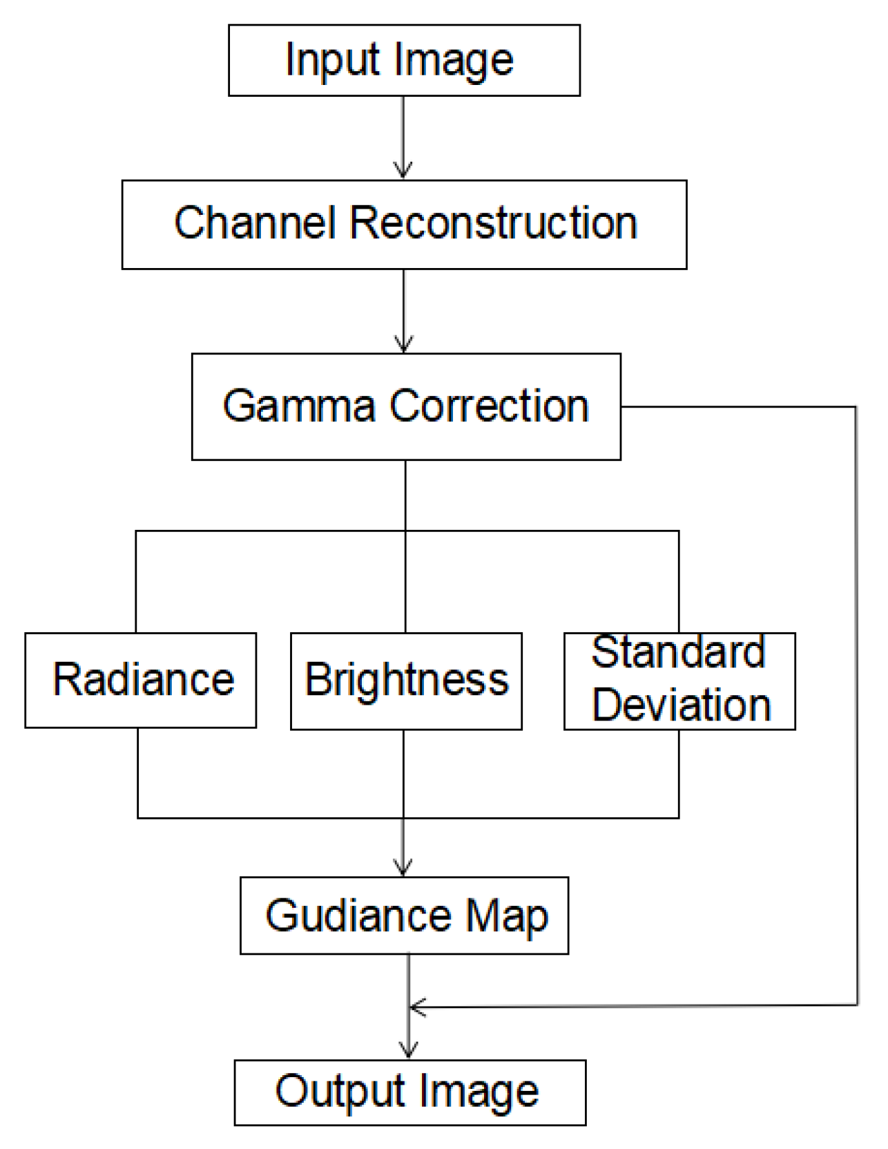
We propose a window algorithm based on tone mapping, which improves the visual effect of the overexposed area in an image by compressing the image’s dynamic range and restoring the information in the exposed area. In this section, we introduce our algorithm in detail. First, the input image is linearized, and the RGB channel of the image is reconstructed; this is a simple preprocessing step. Then, a local gamma correction is performed on the image, and the local contrast of the image is further improved by color compression. The image passes through the previously set window frame, including a series of operations such as guided filtering, after which the final image is output. The algorithmic flow chart is shown in
Figure 1:
The algorithm process mainly involves the following steps: (1) image input; (2) channel reconstruction; (3) gamma correction; (4) generating the guidance map according to Equation (14); (5) restoring the RGB channels in the tone mapped result by Equation (12); (6) resulted image output.
The first step of linearizing the image is crucial. The main reason for operating on the image in linear space is that this provides greater control and predictability regarding the brightness and color domain expansion. In an unknown area, it is difficult to predict how the expansion process will behave. In addition, to recover the scene attributes, such as the mean, geometric average, and standard deviation, we need to estimate the radiance of the scene accurately.
For an input image
,
is the radiance map of the image.
represents the operator.
represents the radiance map of the image after the operation is completed. In short, the core idea of our algorithm is to increase smaller amplitudes and decrease larger amplitudes, this processing step should be conducted in a small area to meet the requirements of amplitude mapping in each pixel neighborhood. The linear function of window
, centered on pixel
i is expressed as follows:
Formula (1) is a complete representation satisfying local constraints. The coefficients and directly affect the local contrast, and represents the slope of the linear function. When , the local contrast is enhanced so that the dark areas in the image are brightened; when , the high-brightness areas in the image are improved. In the overlapping windows with multiple pixels, similar smoothing constraints are enforced in the neighborhood of the center pixel in the smooth area. The contrast is maintained reasonably in the area with abrupt amplitude changes, so there is no need to add constraints.
The defined local linear equation is applied to the window
, and the image is processed by minimizing the solution:
Because of the existence of a trivial solution, we need to add a constraint term to the above formula to make the minimization Formula (2) feasible. According to Formula (1), the coefficient m directly affects the local contrast of the image. We propose guiding its value in each small window to reduce the global contrast while maintaining the image’s information. We support the final objective function as follows:
where
is the default positive number, which is used to guide the processing of the local contrast. The collective
in the image space form the guidance map. By setting an appropriate value for this map, the contrast of the local area can be adjusted correctly (weakening the strong-contrast areas and enhancing the low-contrast areas). The term
is the squared relative error from the guidance map. The term
is used to normalize the difference between
and
. The term
is the weight of the added item. We set its value to 0.1 in the experiments.
The importance of the guidance map is as follows. Although the value affects the local contrast of the image, the accuracy does not need to be very high as the radiance value can be directly modified. In our optimization window, is a weight coefficient that imposes smooth constraints on the guidance map, and the value of this coefficient is very small. The radiance of each pixel is also limited by the linear equation , which effectively maintains the image structure.
3.1. Optimization and Implementation
It is difficult to minimize Formula (3) directly because it contains several unknowns. For each group of linear coefficients
and
, the definitions exist only in a single window, so the minimization problem of Formula (3) can be expressed as:
Through this expression, by computing the partial derivatives of function
for
and
setting them to zero, we obtain the optimal summed solution and obtain the optimal
after solving the linear equation. The calculation process is as follows:
Formulas (5) and (6) can be expressed as a linear relationship:
where
By solving Formula (7), we can obtain:
where
By taking the partial derivatives of the function
to
and setting them to zero, we have:
Combining (8) and (9), we can obtain:
Because of the linearity of Formula (10), it can be simplified as follows:
where
is a Kronecker delta. The optimal solution of Formula (3) is obtained by solving Formula (11). The matrix
in (11) is symmetric and sparse. In each row
of
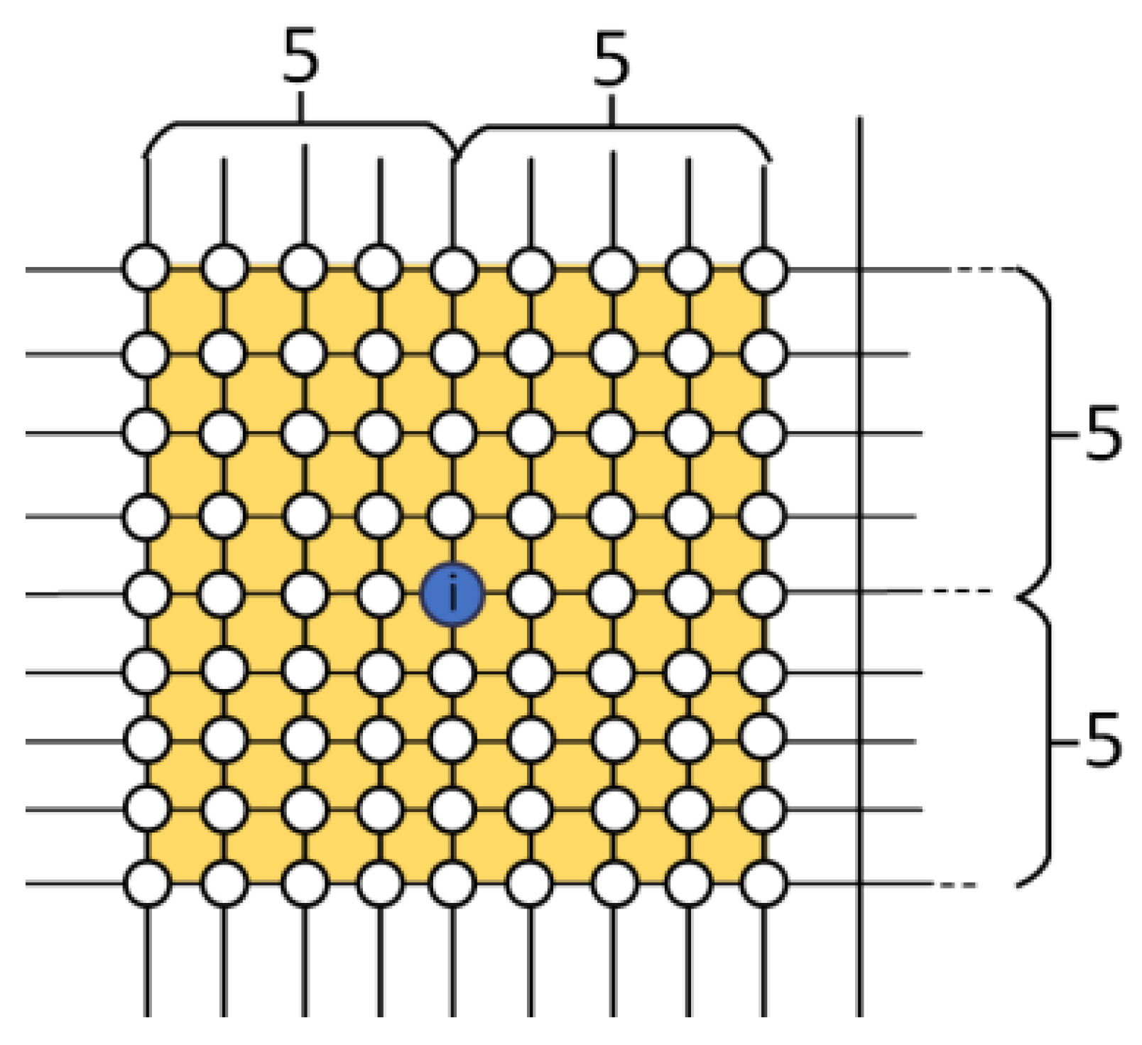
, the number of nonzero elements reaches the area defined according to (11). Given an input image including
pixels, where the size of the window
is set to
,
has fewer than
nonzero elements (a
example is shown in
Figure 2). Mathematically, the minimum possible window size is
, as there are three unknowns in each local window, and at least three linear constraints are needed to make the problem well-posed.
If the image has a medium resolution, we solve the linear system in (11) using symmetric
or the generalized minimum residual method. However, the above method needs several minutes to converge to process an image with a resolution higher than 3024 × 4032. We use a multigrid method [
32] to speed up the processing time, which is the same as the method used in [
33]. In our experiment, it took only a few seconds to produce satisfactory
.
The size of the local window can be adjusted in the system. We set window sizes from to and found that a window size of could produce satisfactory results in terms of image clarity and visual effects. Considering the factors of edge definition and computational complexity, we chose a window in our experiments.
The algorithm above operates on the brightness channel of the input image. After obtaining the radiance map of the image, the RGB channel was reconstructed using the algorithm mentioned in reference [
34]:
where
is one of the RGB color channels of the input image and
is one of the RGB color channels of the output image. The parameter
represents the saturation factor. A larger value of
produces a more saturated result. The introduction of (12) maintains the ratios between the brightness and color channels so that the color of the output image can be similar to that of the original image. In the experiment, we chose
to produce images with natural color.
3.2. Guidance Map Configuration
In the linear optimization framework introduced before, the image processing quality is determined by the guidance map
. We next mainly describe how to obtain an appropriate guidance map
. The coefficient
directly affects the local contrast of the image. To retain the visual information in the image, we reduced the value of
where the local contrast was significant and increased the value of
where the local contrast was slight. The standard deviation
of
is a measure of the local contrast of the image in each window. However,
is inversely proportional to
, which has a bad effect on the results. We defined the guidance map as:
To improve the visual quality of the resulting image, we calculated the Gaussian filtered image and the
of the Gaussian filtered image to reduce noise. In
Figure 3b,c show the radiance map of
and the radiance map of the mean value
, respectively. Since the local mean value
and the radiance map
represent the radiance information of the image, we could see that the information contained in any one of the images was sufficient to contain all the information from the original image completely. If the two factors are added to the guidance image, the local contrast details of the image can be retained as much as possible. We also found that the contrast of the local window radiance is related to the absolute variance. Considering these factors, we add
and
to the guidance map. We redefine
as:
where
is a small weight coefficient. We set it to 0.5 in our experiments to prevent
from being divided by zero. Normally,
,
,
.
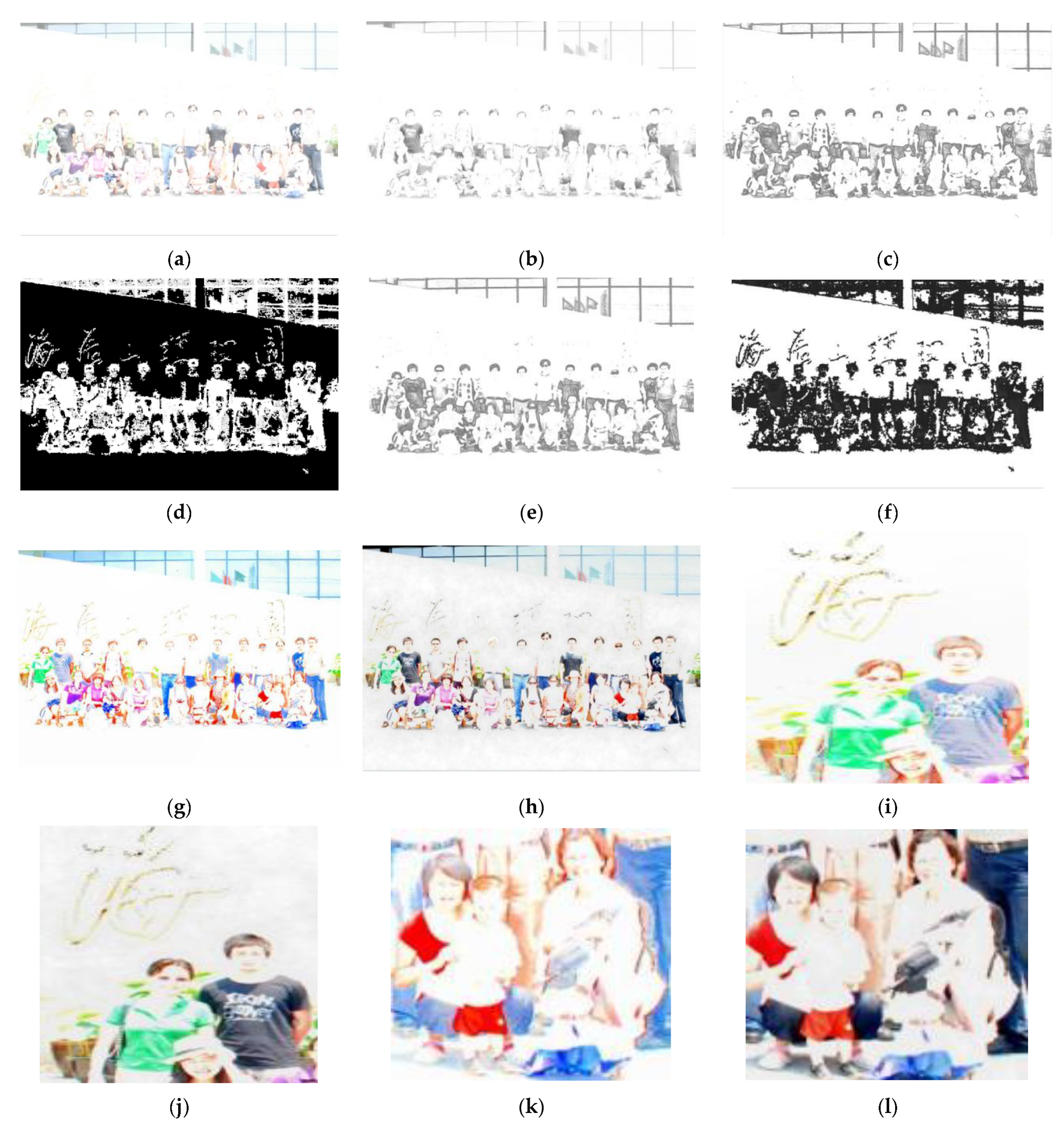
Figure 3 shows the visual image of each parameter and the effect of our newly defined guidance map
on the output image.
Figure 3a is the input image with a large extensive exposure, in which background information can hardly be seen. Only the colors of some personnel’s clothes can be seen in this picture, and the visual effect is inferior.
Figure 3b,c show the image brightness and mean radiance after performing 5 × 5 window processing, respectively.
Figure 3d shows our measure for the local contrast based on the standard deviation of the radiance
. This step can preserve and strengthen the gradients and edges of the image.
Figure 3h shows the image generated by the proposed algorithm, which is produced by the guidance map generated by Formula (7); its visual image is
Figure 3f. We can see that compared with the output image produced by the standard deviation, average value and average brightness of a single image, the visual image of the proposed method contains all the information in the original image, which can significantly improve the restoration quality of the image. Compared with
Figure 3g generated by Formula (6),
Figure 3h generated by our algorithm is better in terms of its color, visual effect and detail processing. The detailed comparison is shown in
Figure 3i–l.
3.3. Parameter Settings
Our settings were based on the following two points. First, the sum of the three affects the global dynamic compression of the input image; a large value makes the resulting image smoother. Second, increasing the value make the compressed edges with higher contrasts more obvious such that more space is left for less prominent areas.
In fact, in our algorithm, minor changes to the sum do not greatly impact the results. The values of these two parameters are small, and the ranges of the values are very small. is fixed at 0.1. For most test images, the default values are and , and most of the tested images can produce visually satisfactory results.
4. Comparative Analysis
To make the algorithm proposed in this paper closer to practical problems, we selected multiple high-brightness license plate images as the processing objects, and we compared our algorithm with several related algorithms proposed by Hui [
35], Khan [
36], Liang [
21] and Xin [
37]. This section includes two parts: part one assesses the restored overexposed images subjectively, and part two objectively compares the results produced by our method and other algorithms.
The sizes of the processed images were 3024 × 4032 pixels in the experiment. To prove the effectiveness of the proposed algorithm, all the algorithms were run on a computer with an Intel Core i5-9400 CPU @ 2.9 GHz (Acer, Taiwan, China), and the compiler software was MATLAB 2019b (9. 7. 0. 1190202, MathWorks, Natick, MA, USA, 2019). In this configuration, the experiments could be completed within 240 seconds.
4.1. Subjective Analysis
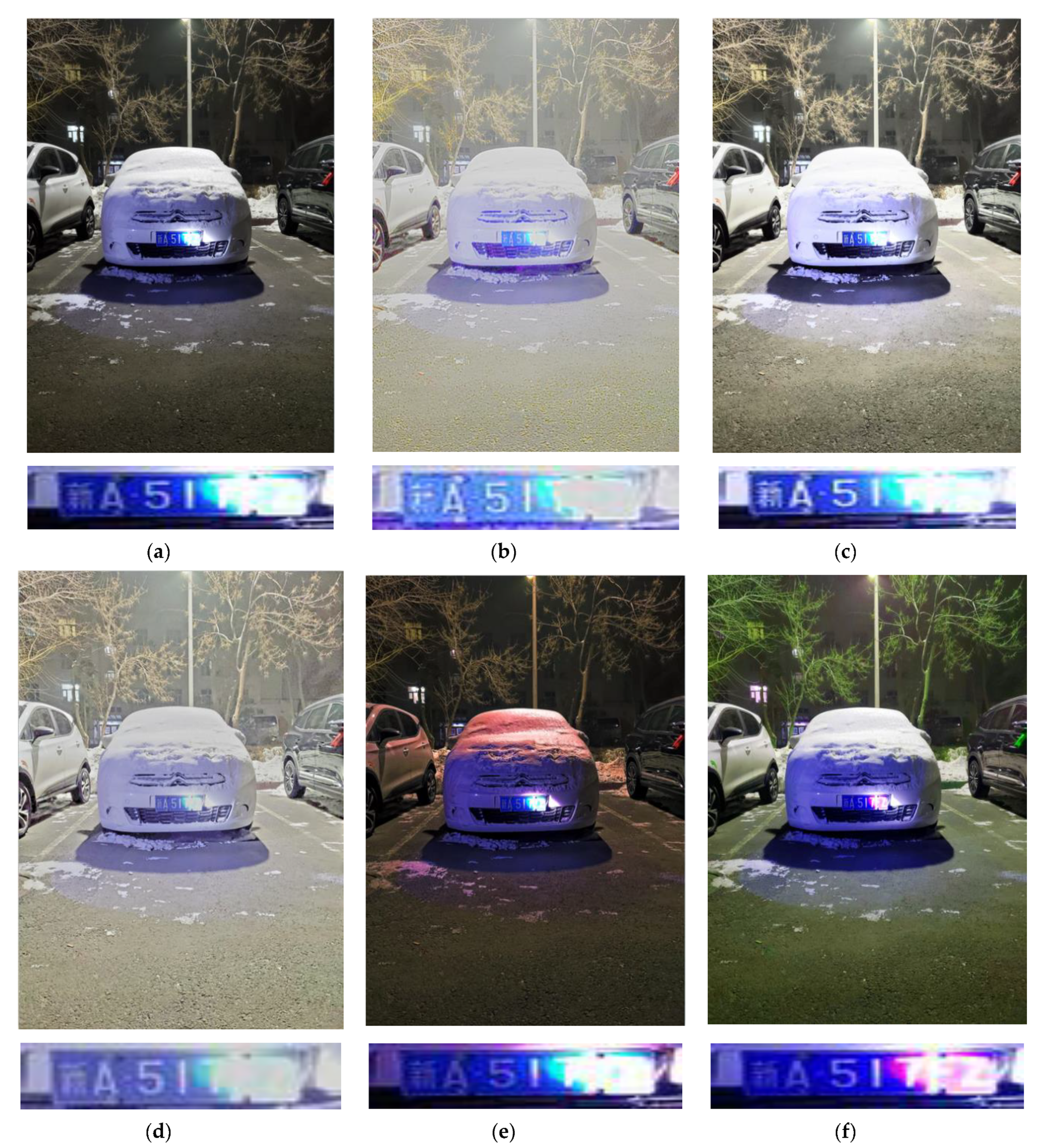
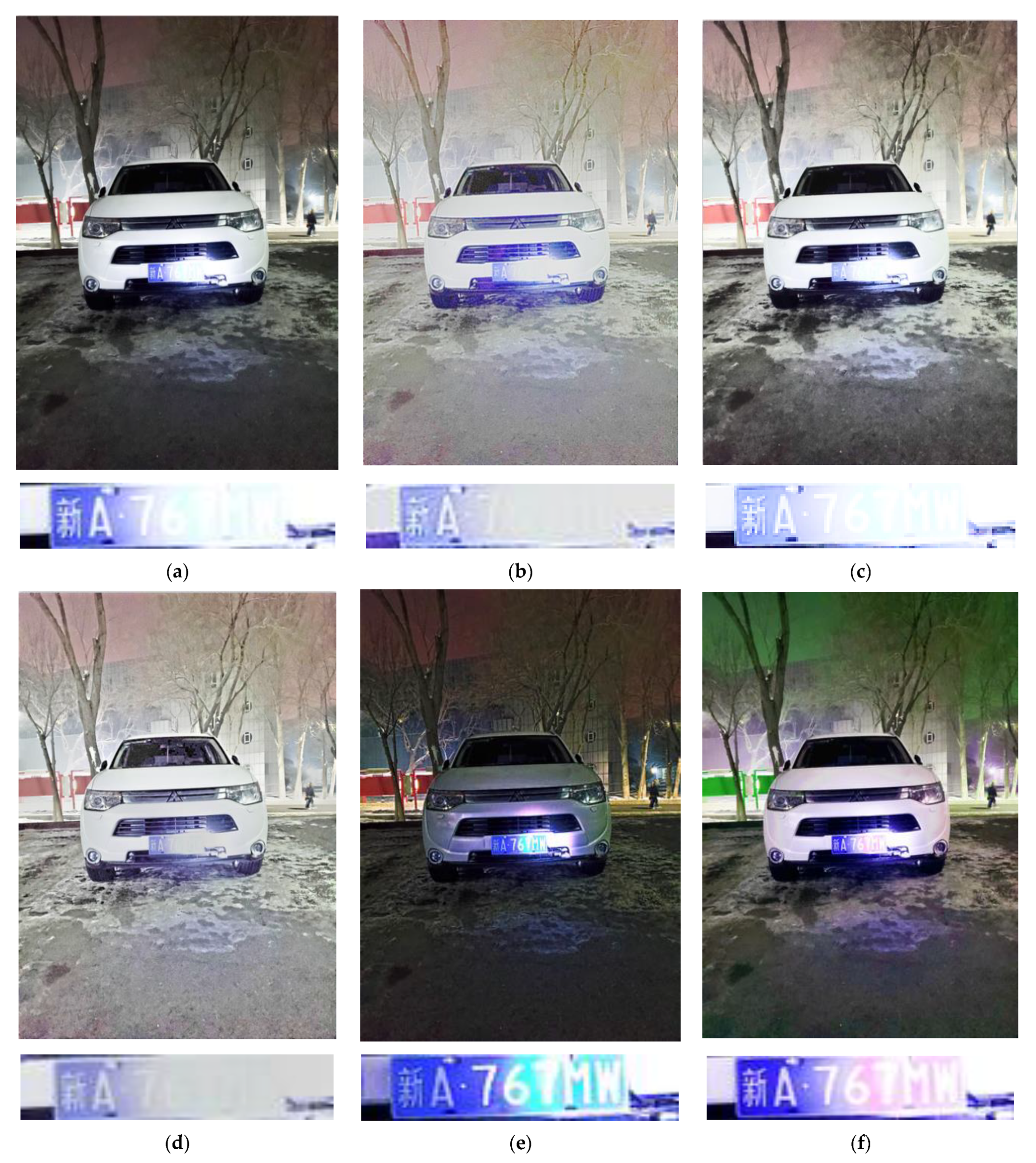
In this part, we mainly analyze the experimental results. As shown in
Figure 4,
Figure 5,
Figure 6,
Figure 7, the representative algorithms developed by Hui [
35], Khan [
36], Liang [
21] and Xin [
37] were compared with the algorithm proposed in this paper on different images.
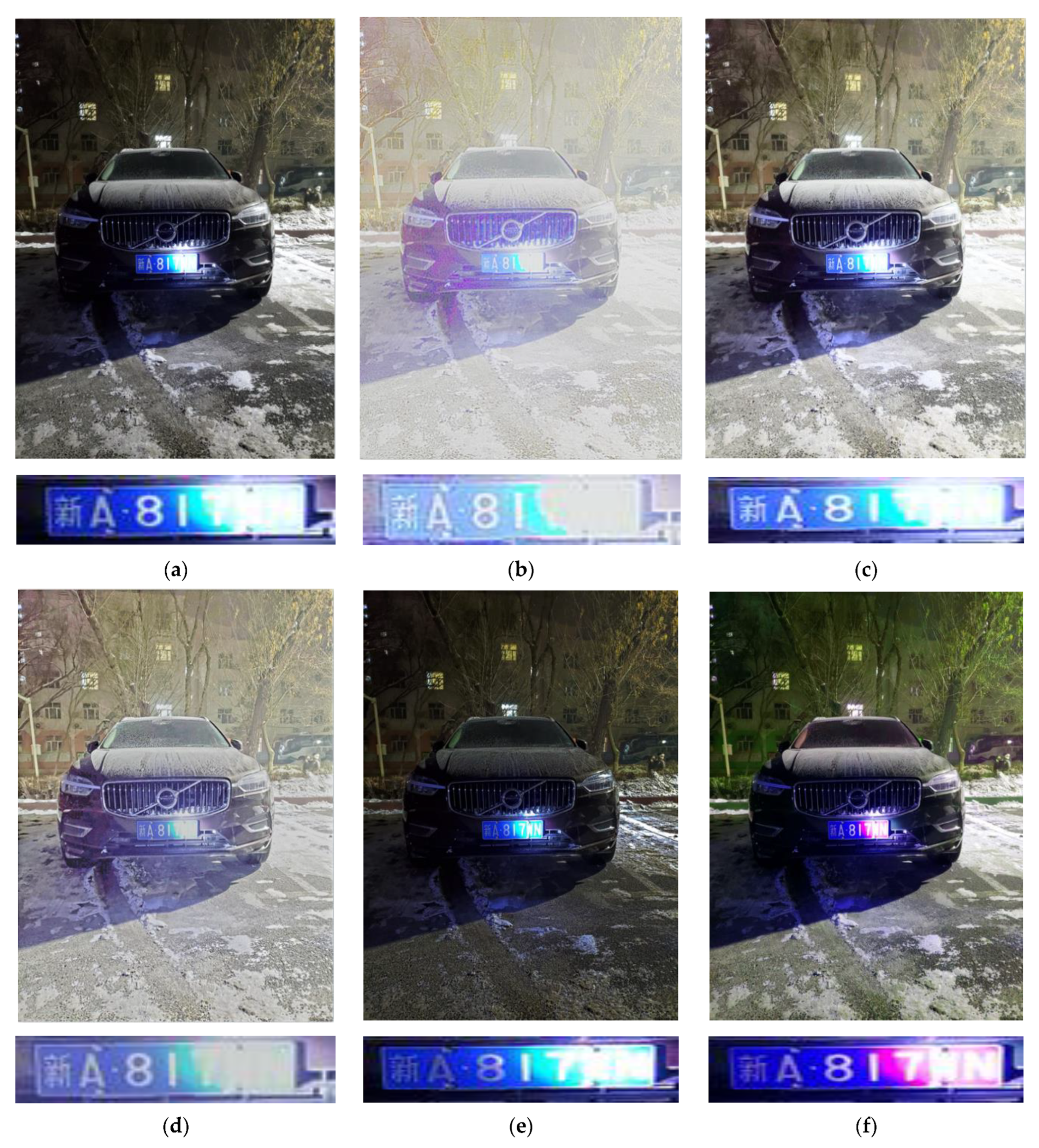
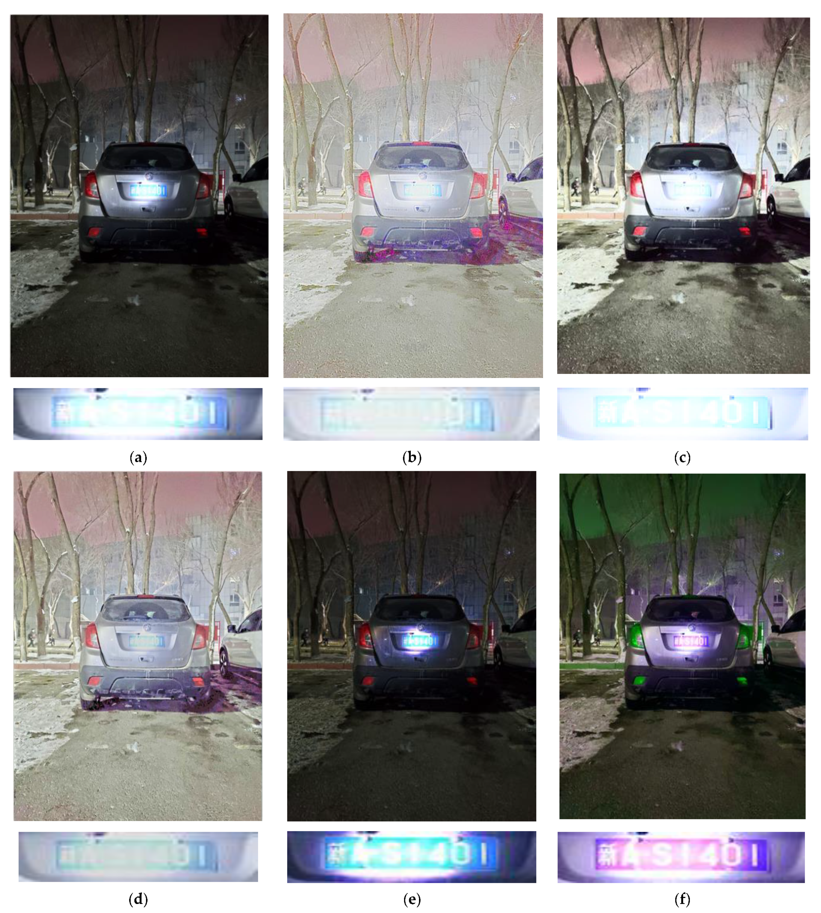
From the perspective of visual effects, as shown in
Figure 6e and
Figure 7e, the algorithm of Xin [
37] also improved the high-brightness area. Still, our algorithm had greater advantages in terms of the overall contrast of the image and the details of the scene. However, the other algorithms could not effectively recover the information of the key area for all the experimental images. The results showed that the effect of our algorithm regarding key information recovery was pronounced. Although the image’s hue was slightly green, especially as shown in
Figure 7f (our algorithm made the vehicle tail lamp change from red to green), the critical exposure area information was recovered. To the overall improvement of the image, the visual effect was ideal, reaching expectations.
By observing the experimental results, we could find that the brightness of the original image with much light was improved significantly, and the information of the local area with much light was effectively restored. Compared with the image processed by the algorithm, the information of the high-brightness area was not recovered well.
4.2. Objective Analysis
We calculated four objective indicators, including the structural similarity (SSIM), peak signal-to-noise ratio (PSNR), image information entropy (H) and executive time. The bigger the first three indicators, the better. The specific values are shown in
Table 1,
Table 2,
Table 3,
Table 4,
Table 5 below.
Table 1 shows the objective values of
Figure 4.
Table 2 shows the objective values of
Figure 5.
Table 3 shows the objective values of
Figure 6.
Table 4 shows the objective values of
Figure 7.
As shown in the tables, we can see that our algorithm ranked first, especially in terms of the SSIM and PSNR. Our algorithm was also better than that of Xin [
37] in terms of the SSIM. SSIM is an index used to measure the similarity of two images. We got images with different illumination intensity at different times from the video, including lossless images and distorted images. We processed the high-brightness images through the proposed algorithm. Comparing the resulting image with the lossless, we evaluated the quality of image restoration. SSIM reflects the comprehensive similarity of two images in brightness, contrast and structure. By averaging the objective indicators of the 50 high-brightness video images, the average PSNR of our algorithm was 29.53, which was 7.22 higher than that of the algorithm by Xin [
37]. In terms of the PSNR, the proposed algorithm was better than the algorithm of Xin [
37]. This shows that after compression, the image quality was better than that obtained by the algorithm of Xin [
37]. The larger the PSNR value, the smaller the image distortion. “H” reflects the average amount of information in the image and demonstrates the richness of image information from the perspective of information theory. Generally, the bigger the H value, the better. Our method ranked second in H. For the time part, because the generation of a guidance map takes a long time, our algorithm was not dominant in all comparative experiments. This will be our next optimization direction.
In summary, by combining a subjective evaluation and an objective analysis, we can conclude that the proposed algorithm could effectively recover the exposure area information from high-brightness video images with sound visual effects, and the objective indicators were much better than those produced by the compared algorithms.


