
Tooth Position Determination by Automatic Cutting and Marking of Dental Panoramic X-ray Film in Medical Image Processing

 , , , , ,
Abstract
:1. Introduction
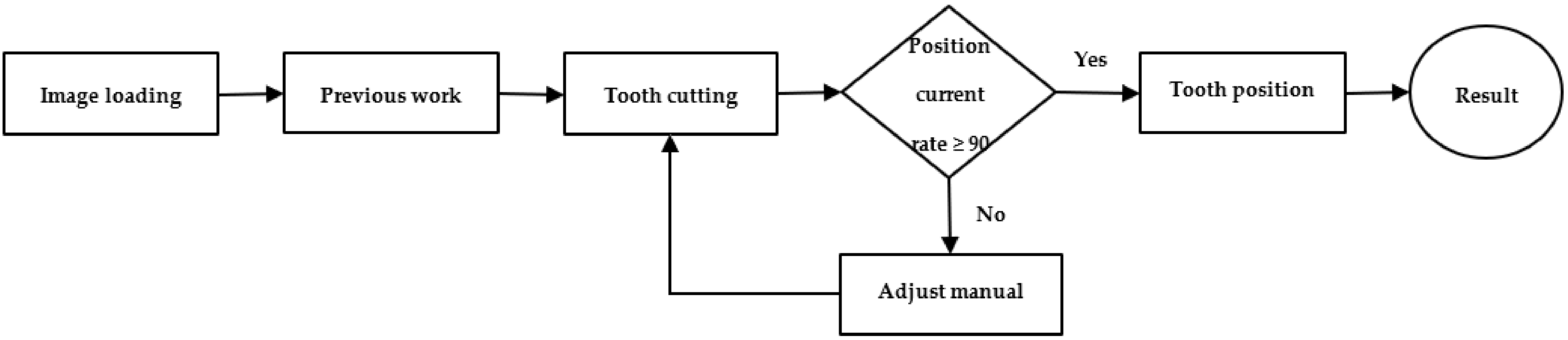
2. Method
2.1. Previous Works
2.1.1. Sharpening
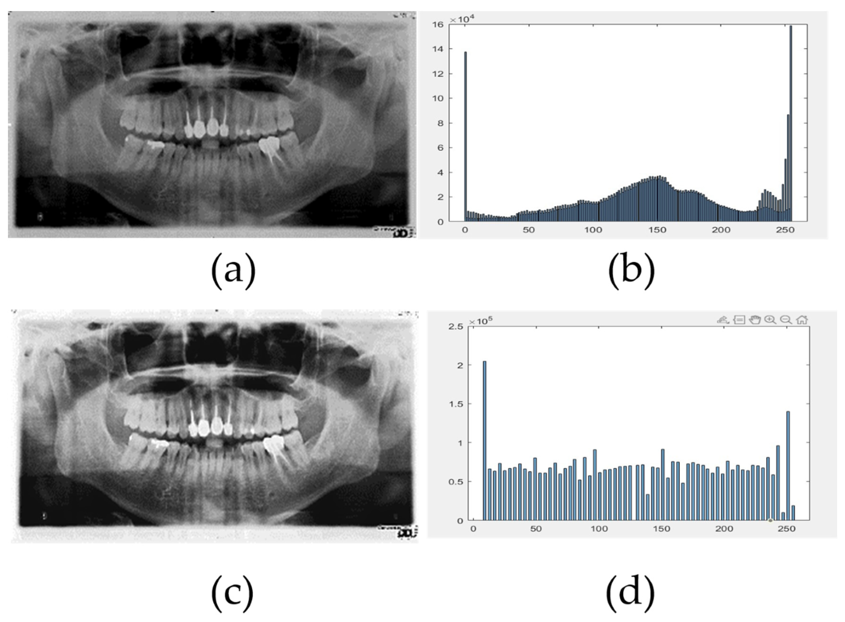
2.1.2. Image Contrast Adjustment
- For any value of r in the interval of 0 to 1, change according to the inequality .
- The above transformation must meet the following conditions:
- (1)
- For 0 ≤ r ≤ 1, there are 0 ≤ s ≤ 1.
- (2)
- Within the interval, is a uniform increase for a single value.
- (3)
- The reverse transformation from s to r is , where by .
- (4)
- The inverse transformation also meets criteria (1) and (2).
2.1.3. Flat-Field Correction
- (1)
- Non-uniform illumination;
- (2)
- Inconsistent response between the center and edge of the lens;
- (3)
- The image devices not responding consistently to each response;
- (4)
- Fixed image background noise.
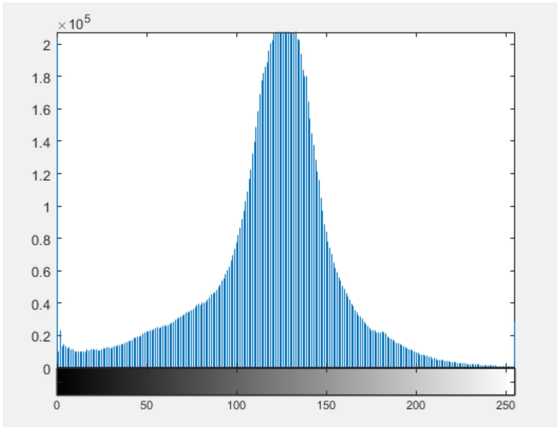
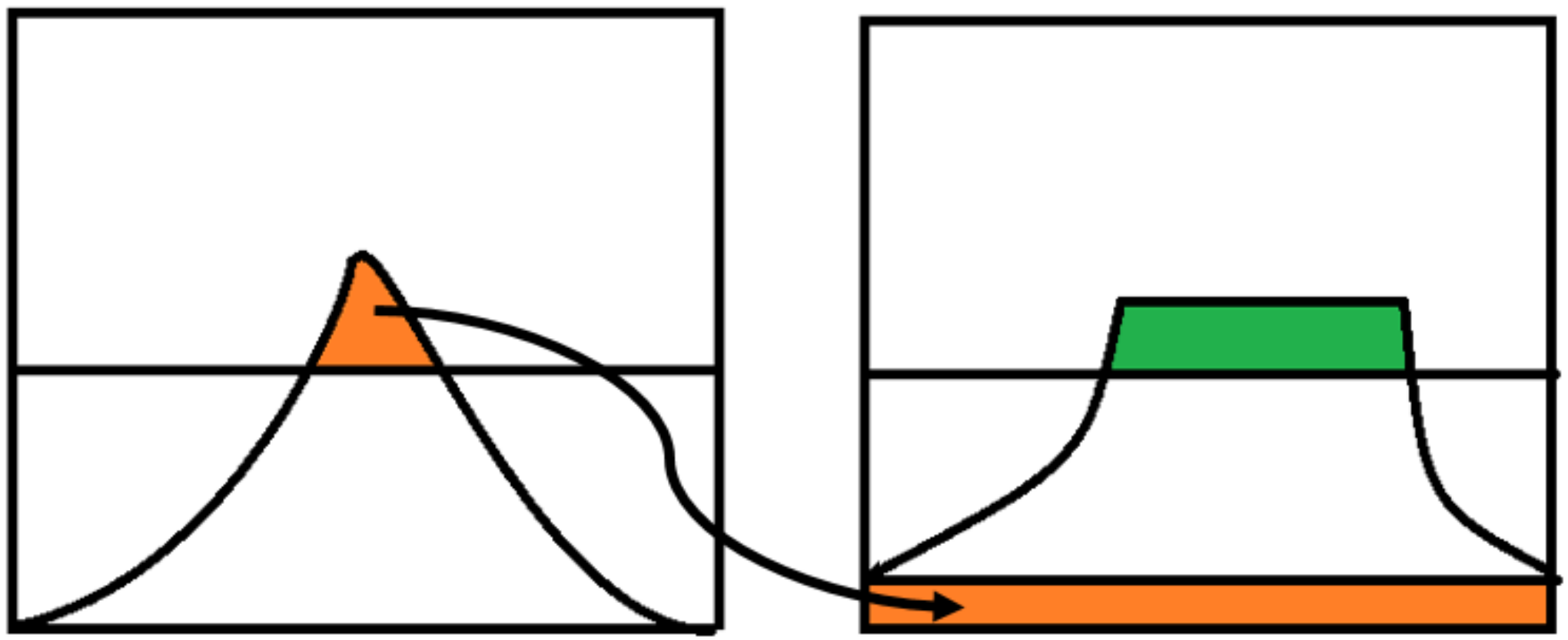
2.1.4. Adaptive Histogram Equalization
- (1)
- If the amplitude is higher than CL, it is used directly as CL;
- (2)
- If the amplitude is between Upper and CL, fill it to CL;
- (3)
- If the amplitude is lower than Upper, fill L pixels directly.
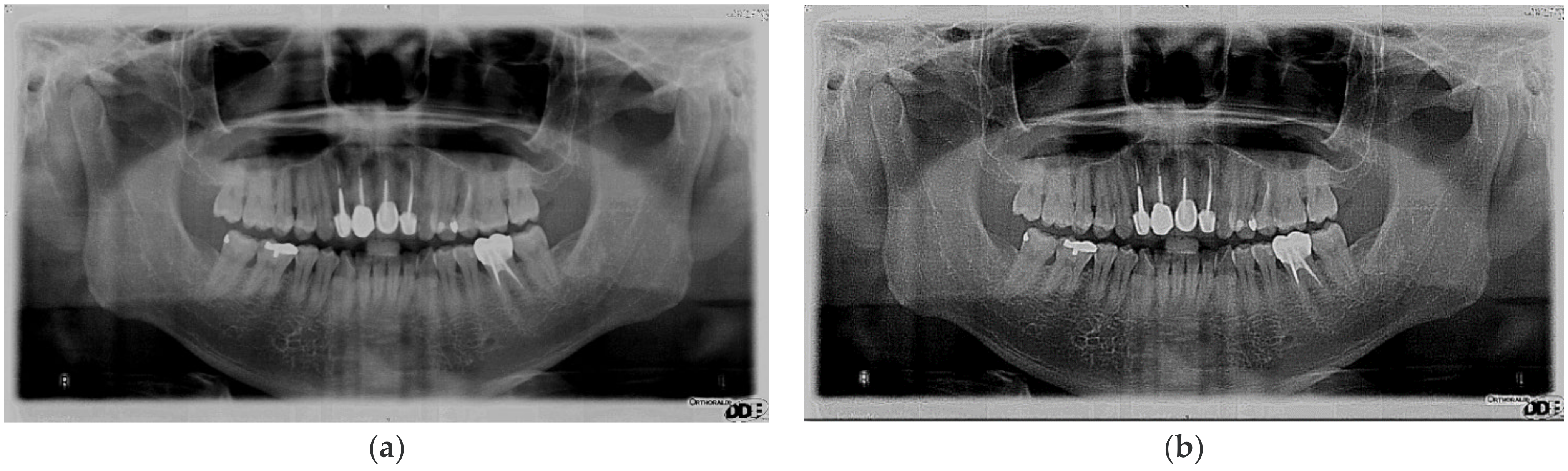
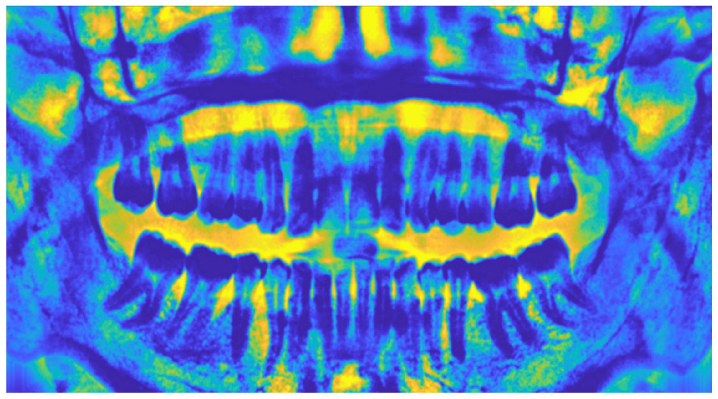
2.2. Image Segmentation
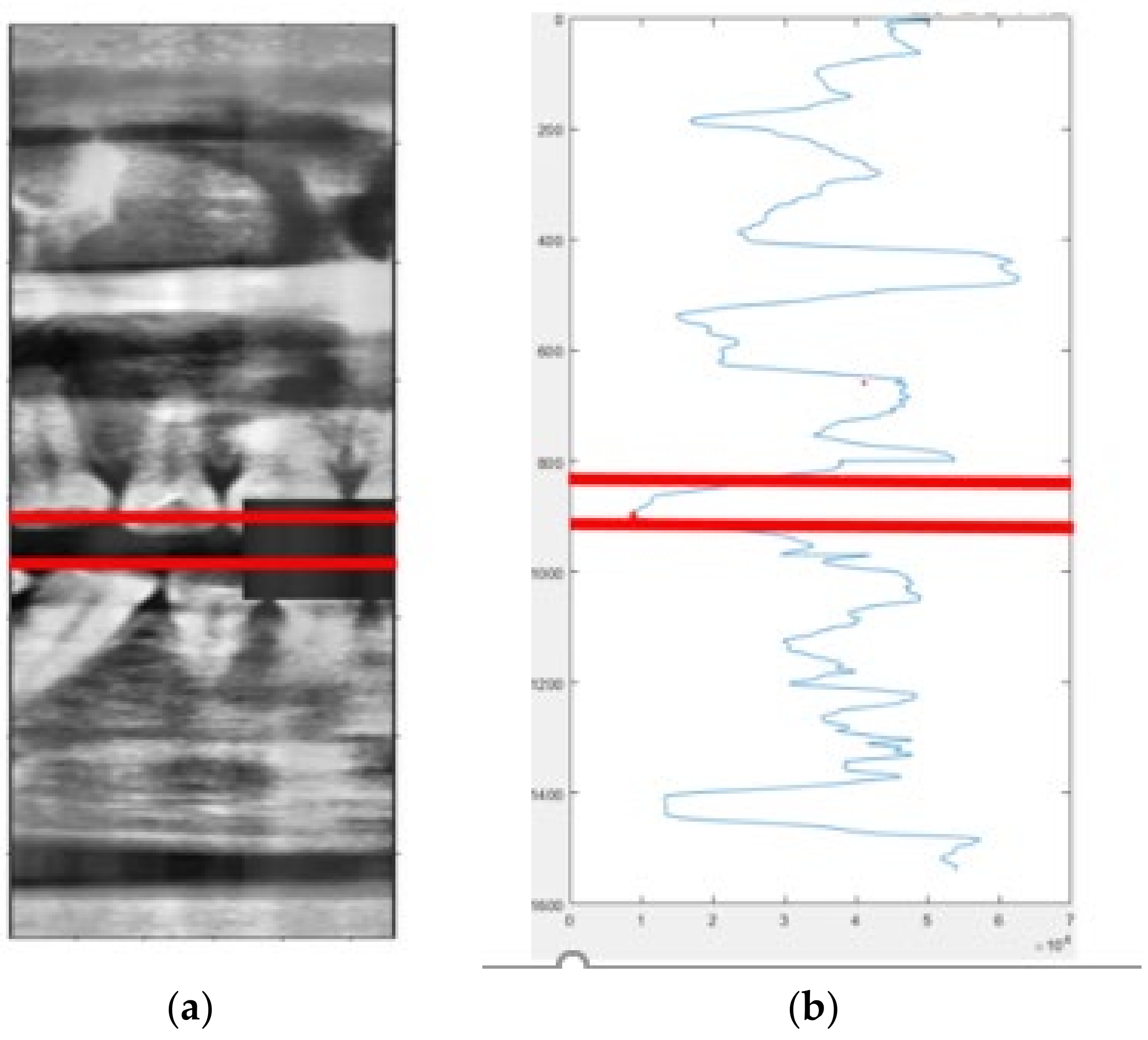
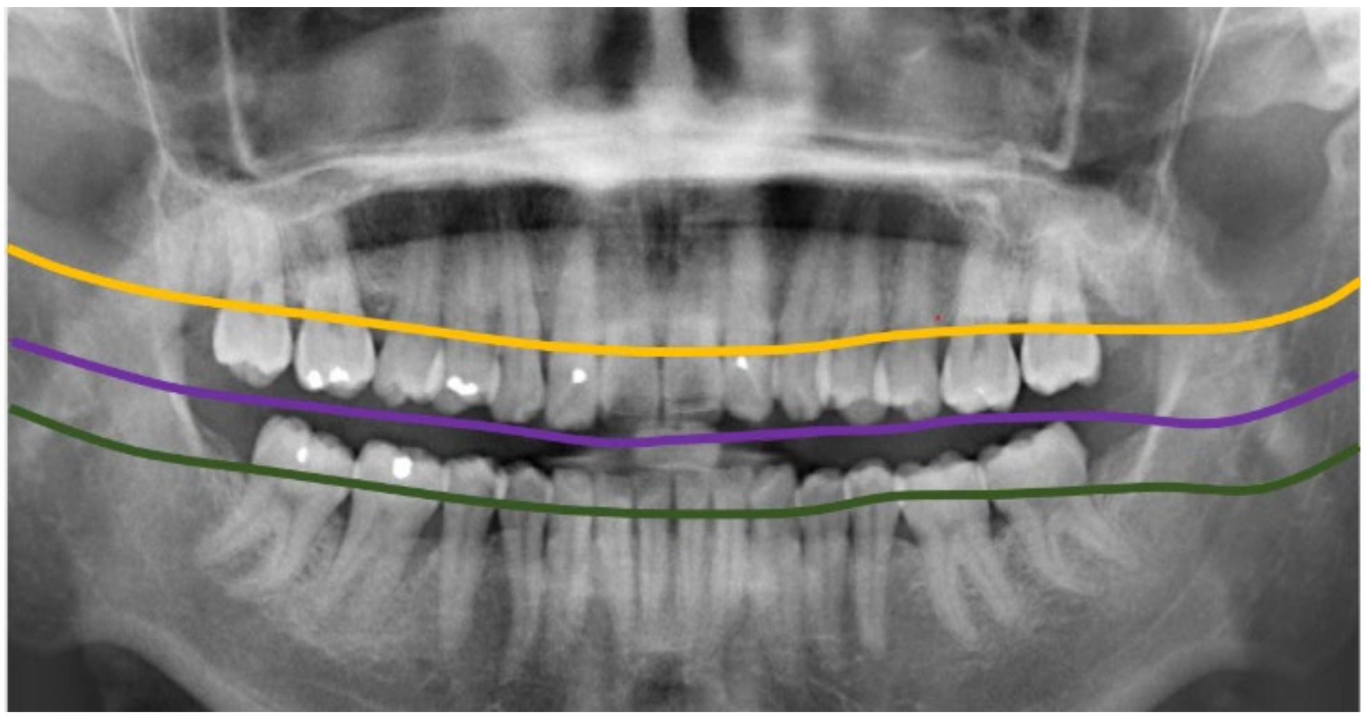
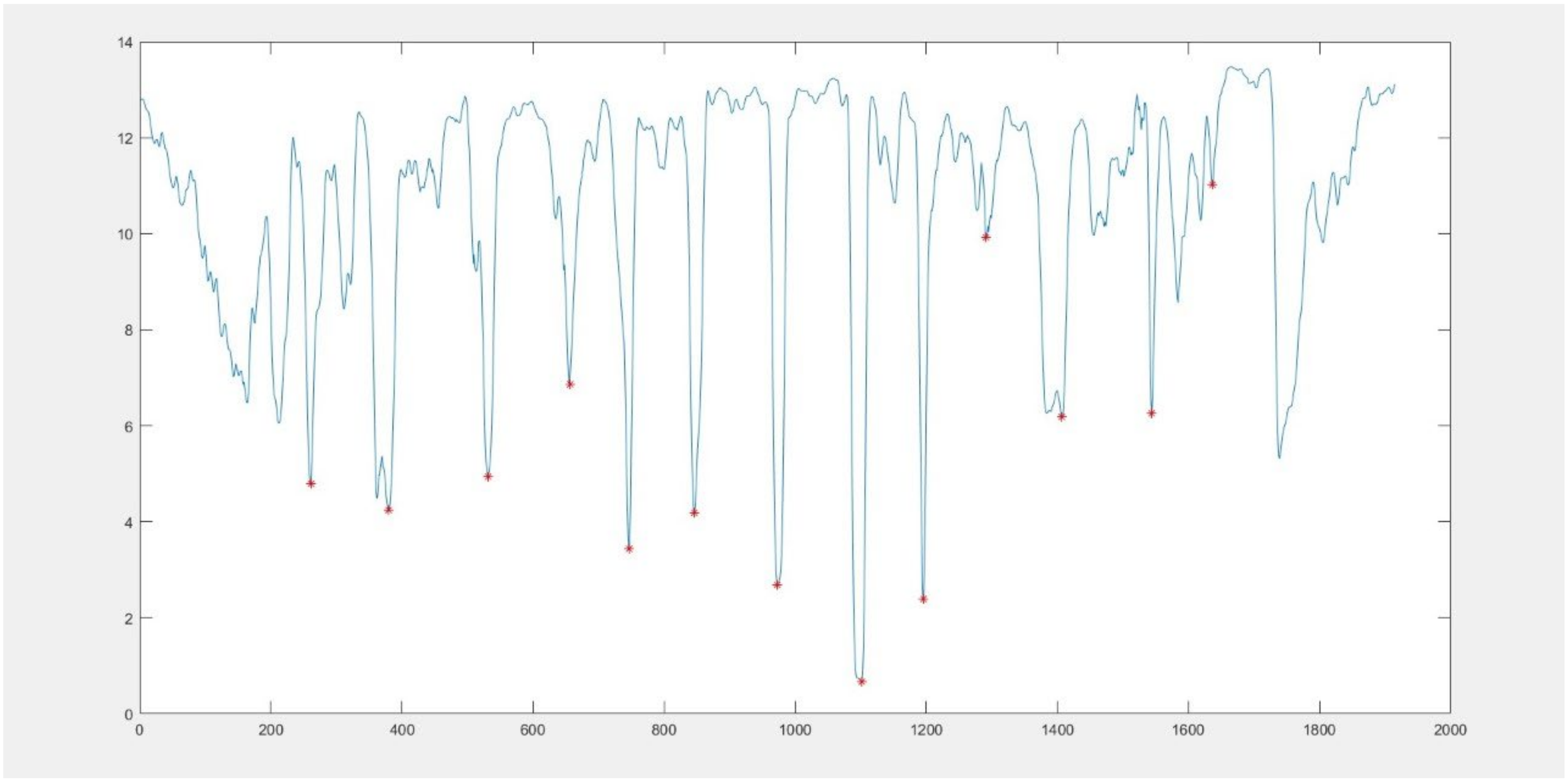
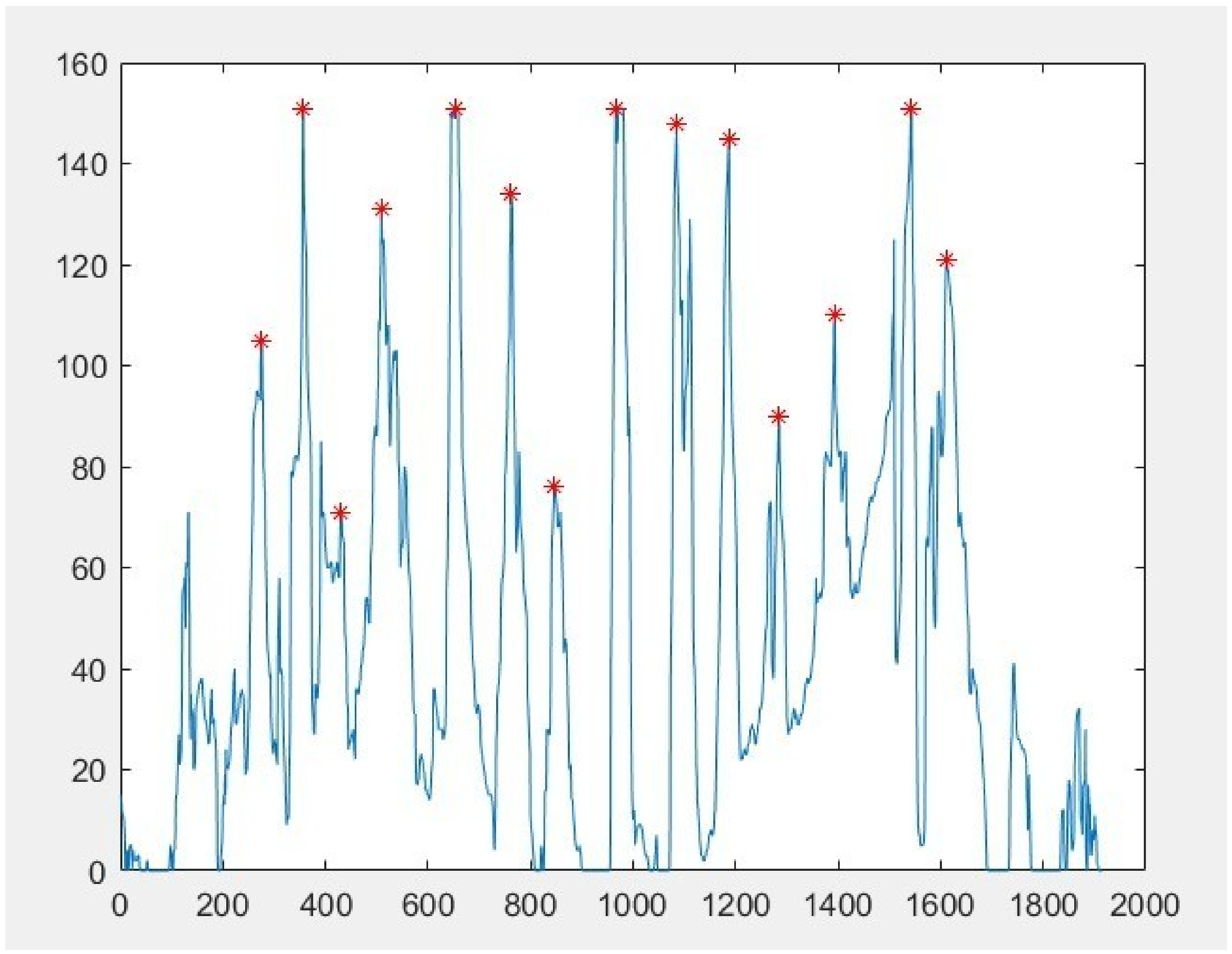
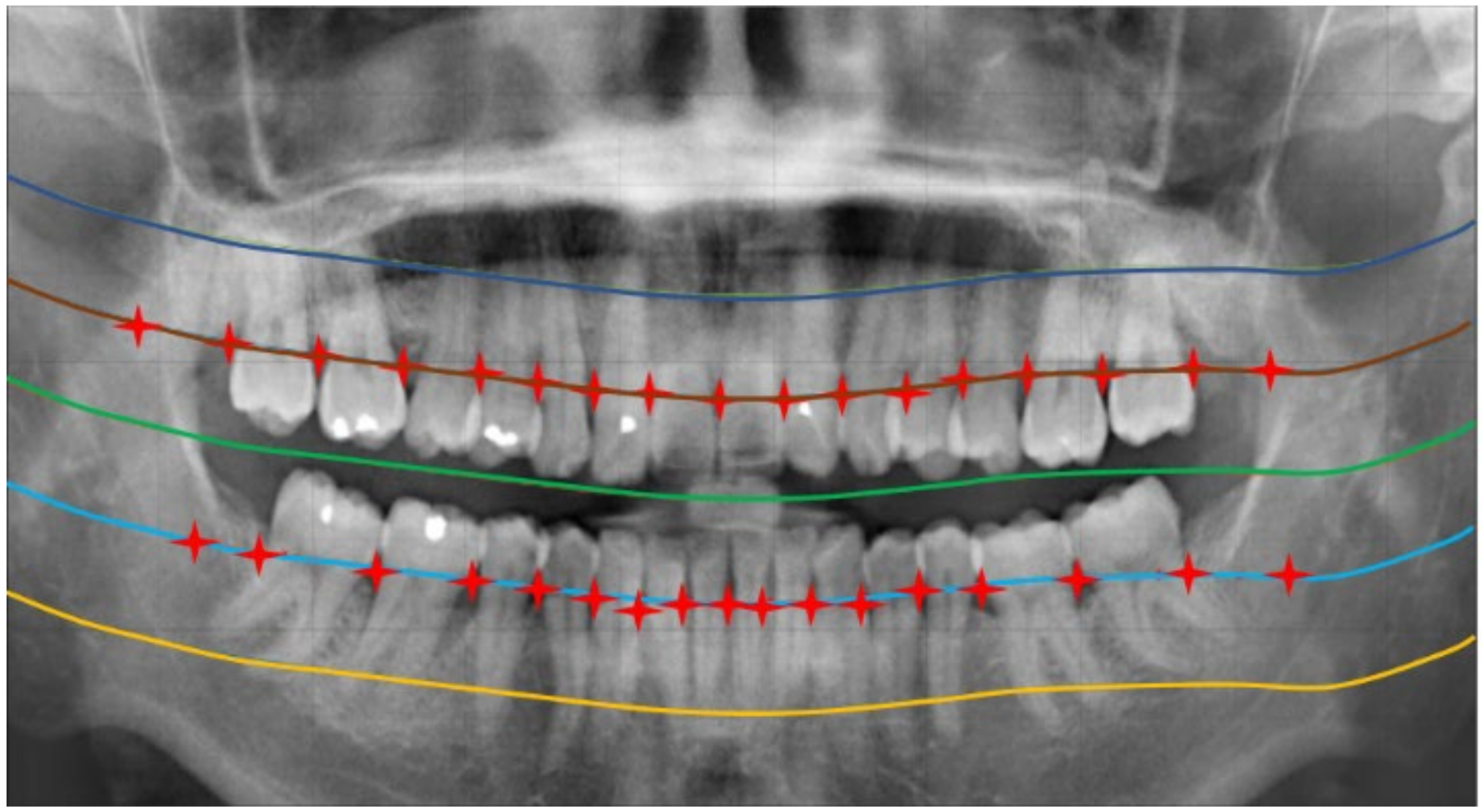
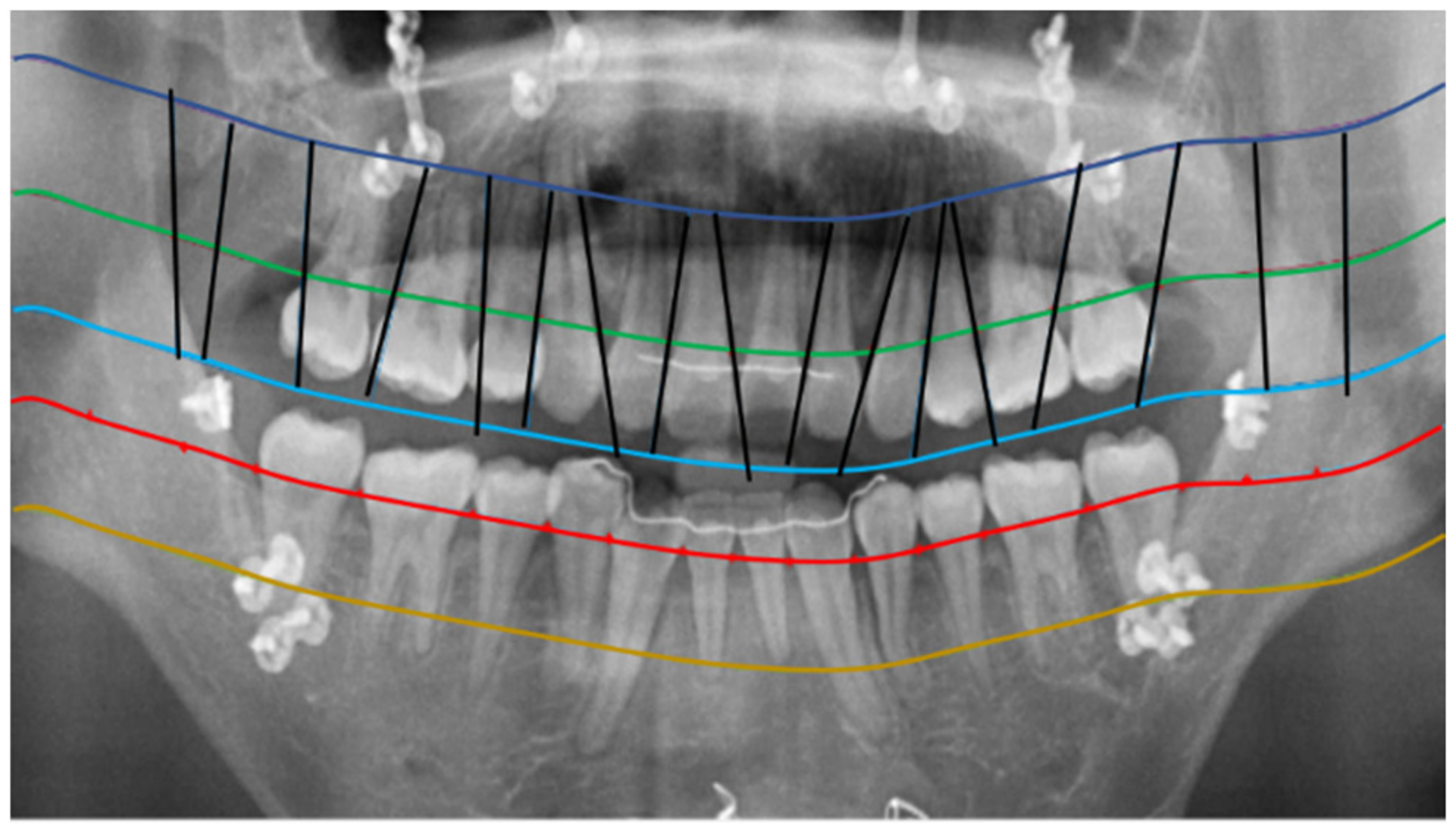
2.2.1. Curve of the Mouth
2.2.2. Curve Adjustment
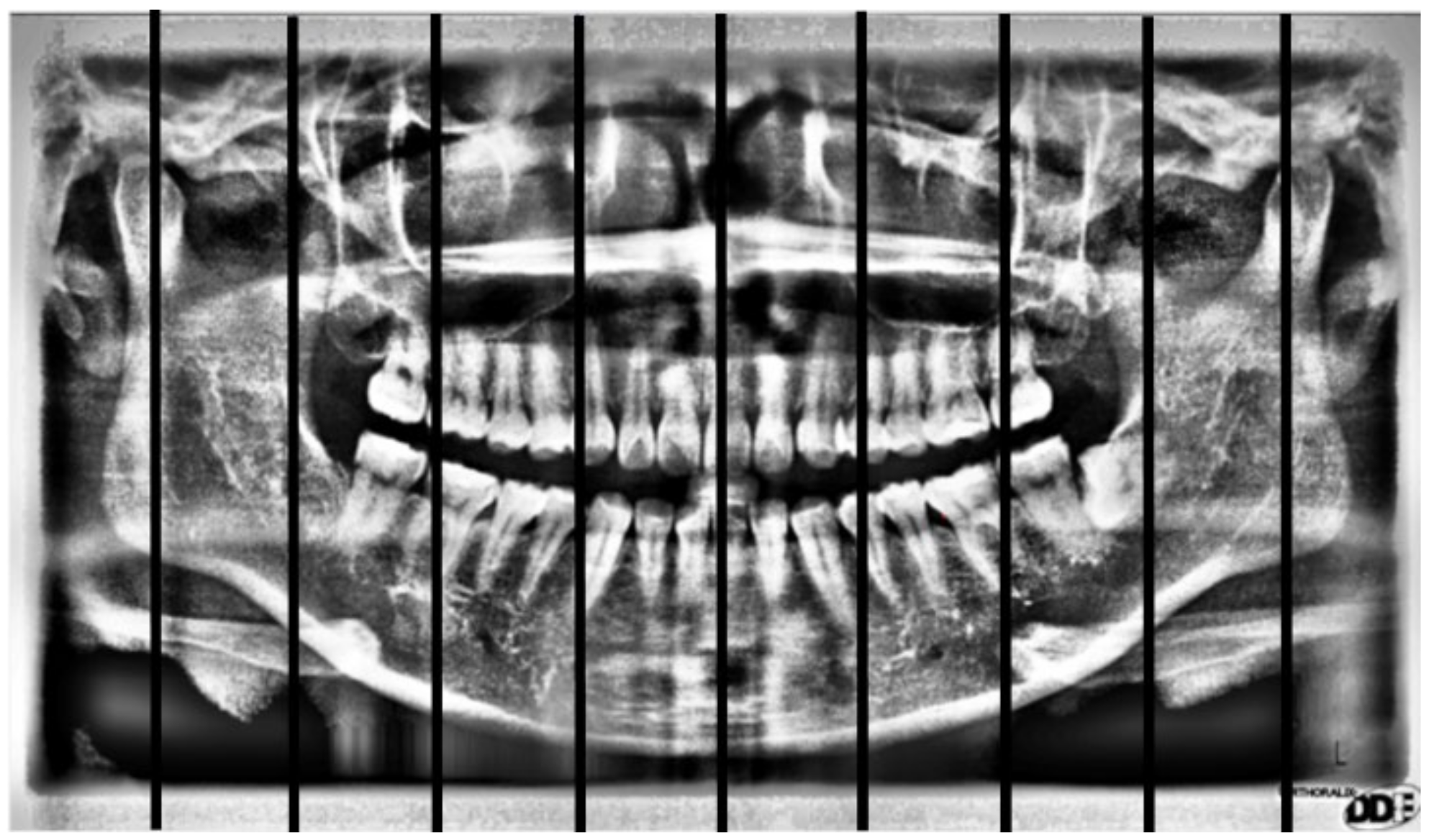
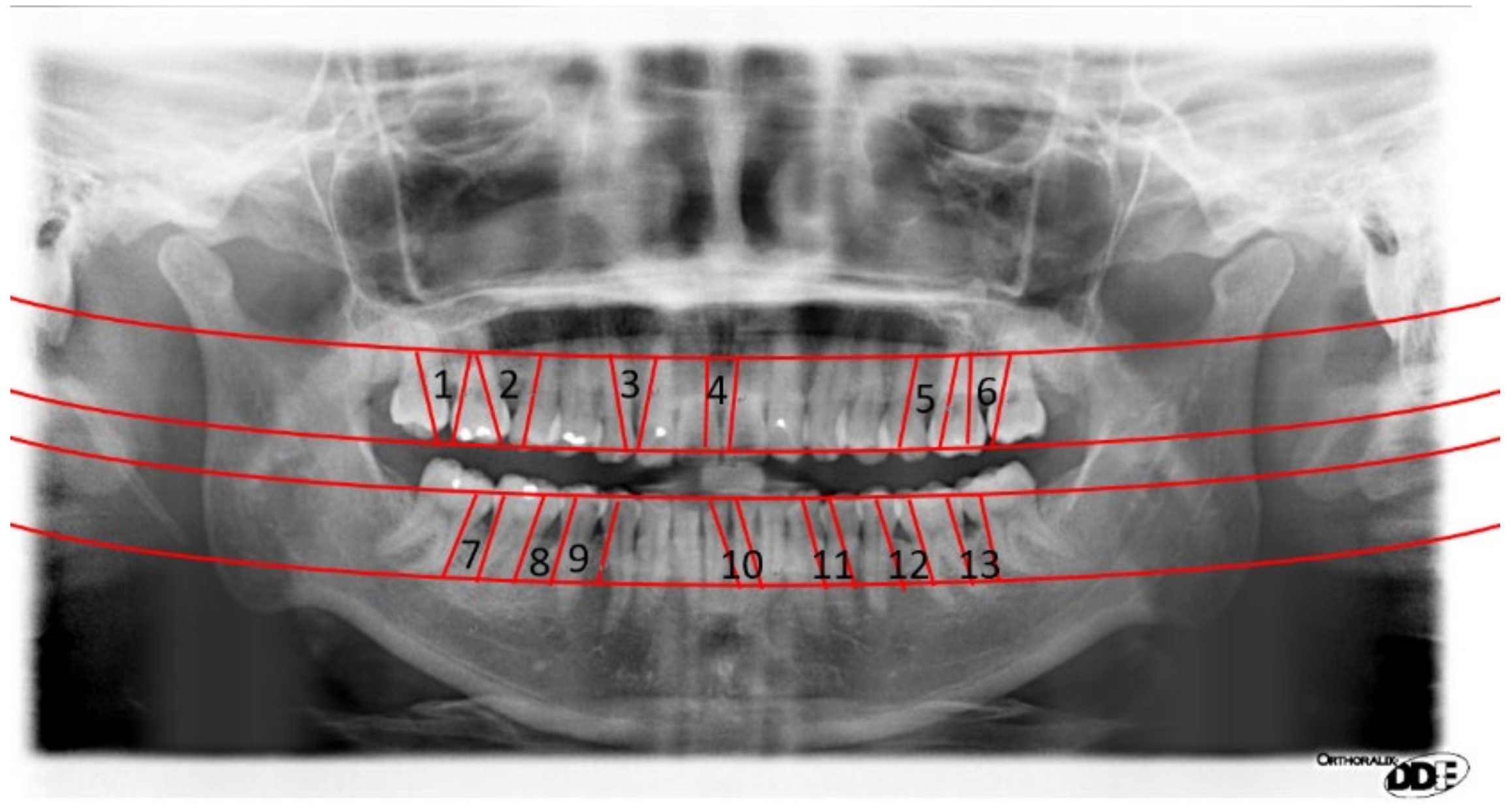
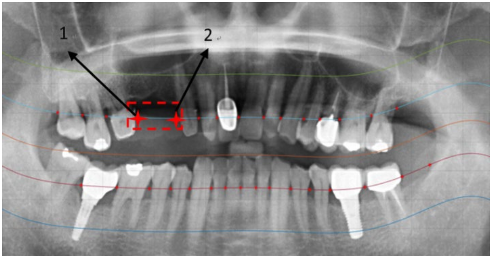
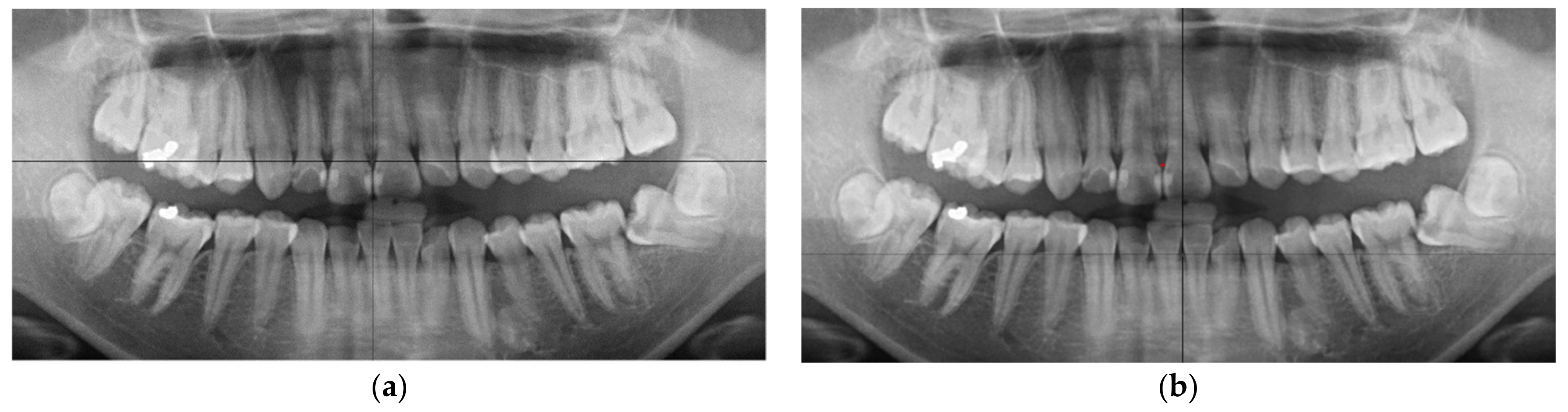
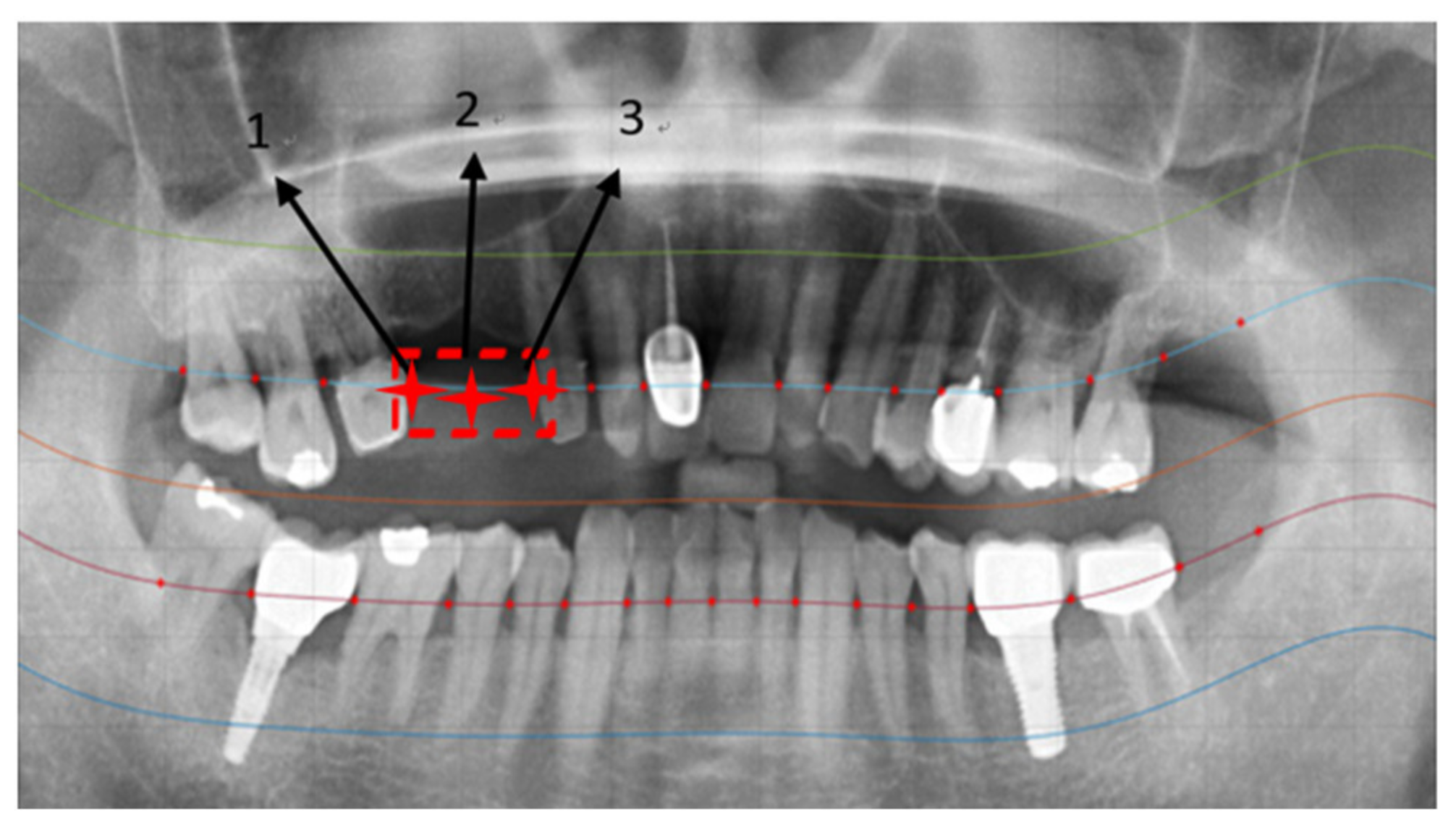
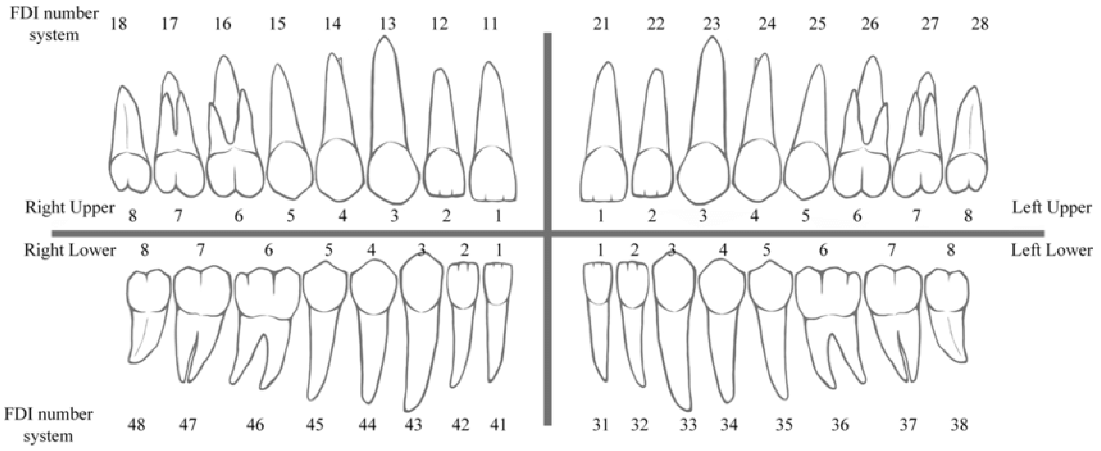
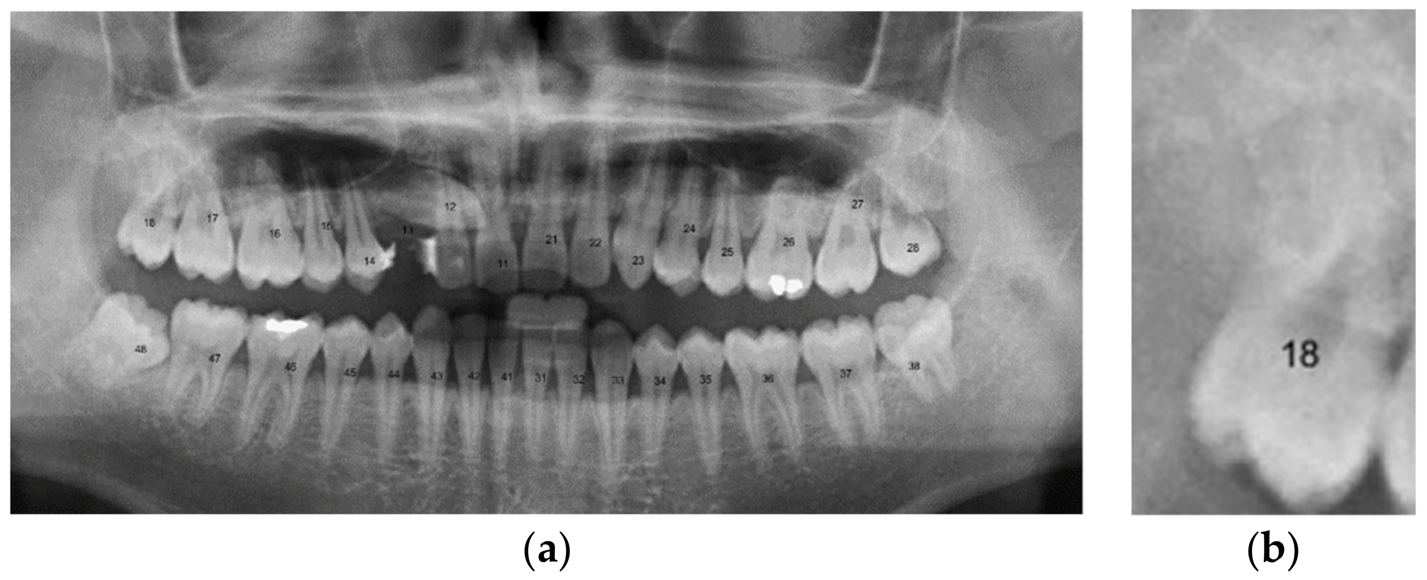
2.2.3. Positioning Numbers
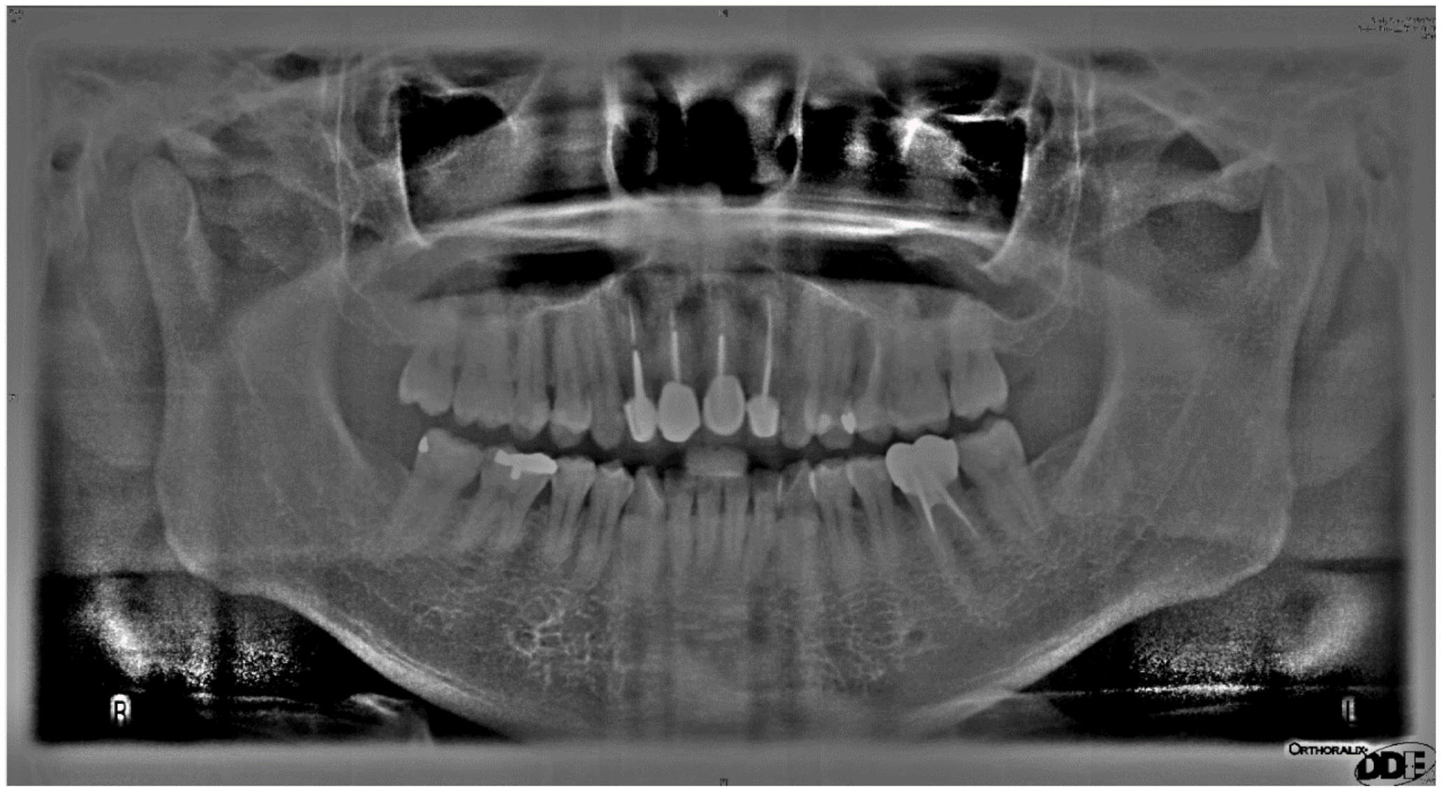
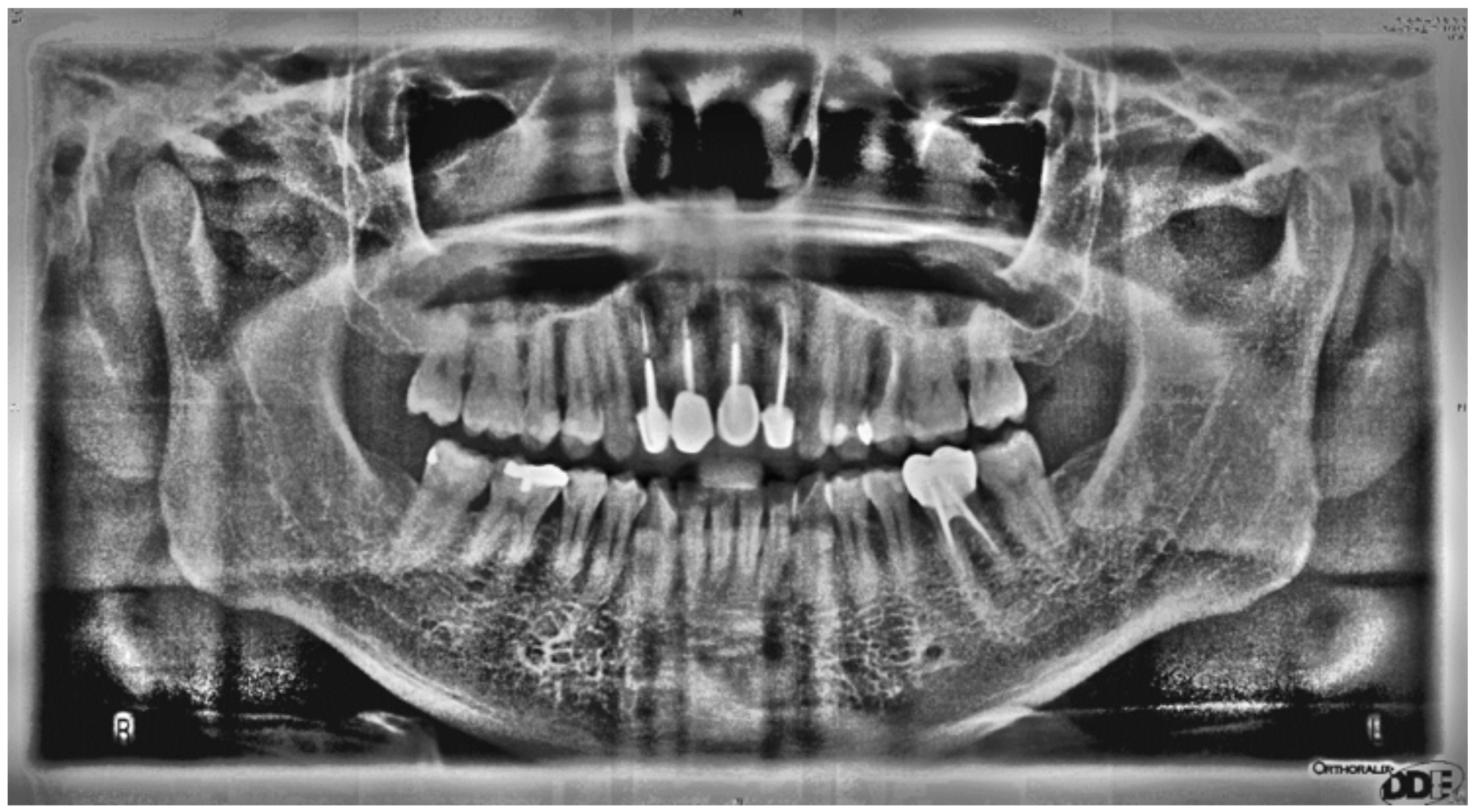
3. Results
4. Conclusions
Author Contributions
Funding
Institutional Review Board Statement
Informed Consent Statement
Data Availability Statement
Acknowledgments
Conflicts of Interest
References
- Visser, W.; Schwaninger, A.; Hardmeier, D.; Flisch, A.; Costin, M.; Vienne, C.; Sukowski, F.; Hassler, U.; Dorion, I.; Marciano, A.; et al. Automated comparison of X-ray images for cargo scanning. In Proceedings of the 2016 IEEE International Carnahan Conference on Security Technology (ICCST), Orlando, FL, USA, 24–27 October 2016; pp. 1–8. [Google Scholar] [CrossRef]
- Amisha, M.P.; Pathania, M.; Rathaur, V.K. Overview of artificial intelligence in medicine. J. Fam. Med. Prim. Care 2019, 8, 2328–2331. [Google Scholar] [CrossRef] [PubMed]
- Shan, T.; Tay, F.; Gu, L. Application of artificial intelligence in dentistry. J. Dent. Res. 2021, 100, 232–244. [Google Scholar] [CrossRef] [PubMed]
- Khanagar, S.B.; Al-Ehaideb, A.; Maganur, P.C.; Vishwanathaiah, S.; Patil, S.; Baeshen, H.A.; Sarode, S.C.; Bhandi, S. Developments, application, and performance of artificial intelligence in dentistry–A systematic review. J. Dent. Sci. 2021, 16, 508–522. [Google Scholar] [CrossRef] [PubMed]
- Cantu, A.G.; Gehrung, S.; Krois, J.; Chaurasia, A.; Rossi, J.G.; Gaudin, R.; Elhennawy, K.; Schwendicke, F. Detecting caries lesions of different radiographic extension on bitewings using deep learning. J. Dent. 2020, 100, 103425. [Google Scholar] [CrossRef] [PubMed]
- Schwendicke, F.; Golla, T.; Dreher, M.; Krois, J. Convolutional neural networks for dental image diagnostics: A scoping review. J. Dent. 2019, 91, 103226. [Google Scholar] [CrossRef]
- American Dental Association. Dental Radiographic Examinations: Recommendations for Patient Selection And Limiting Radiation Exposure; American Dental Association, U.S. Department of Health and Human Services: Washington, DC, USA; FDA: Silver Spring, MD, USA, 2012.
- Perschbacher, S. Interpretation of panoramic radiographs. Aust. Dent. J. 2012, 57, 40–45. [Google Scholar] [CrossRef] [PubMed]
- White, S.C.; Pharaoh, M.J. Oral Radiology: Principles and Interpretation, 7th ed.; Mosby: St. Louis, MO, USA, 2014. [Google Scholar]
- Chen, H.; Zhang, K.; Lyu, P.; Li, H.; Zhang, L.; Wu, J.; Lee, C.-H. A deep learning approach to automatic teeth detection and numbering based on object detection in dental periapical films. Sci. Rep. 2019, 9, 1–11. [Google Scholar] [CrossRef] [PubMed] [Green Version]
- Shakir, H.; Ahsan, S.T.; Faisal, N. Multimodal medical image registration using discrete wavelet transform and Gaussian pyramids. In Proceedings of the 2015 IEEE International Conference on Imaging Systems and Techniques (IST), Macau, China, 16–18 September 2015; pp. 1–6. [Google Scholar] [CrossRef]
- Li, X.; Zhang, Y.; Cui, Q.; Yi, X. Tooth-marked tongue recognition using multiple instance learning and CNN features. IEEE Trans. Cybern. 2019, 49, 380–387. [Google Scholar] [CrossRef] [PubMed]
- Yu, Y.; Wang, J. Beam hardening-respecting flat field correction of digital X-ray detectors. In Proceedings of the 2012 19th IEEE International Conference on Image Processing, Orlando, FL, USA, 30 September–3 October 2012; pp. 2085–2088. [Google Scholar] [CrossRef]
- Wanat, R. A Problem of Automatic Segmentation of Digital Dental Panoramic X-ray Images for Forensic Human Identification. Available online: https://old.cescg.org/CESCG-2011/papers/Szczecin-Wanat-Robert.pdf (accessed on 5 December 2021).
- Kim, G.; Lee, J.; Seo, J.; Lee, W.; Shin, Y.-G.; Kim, B. Automatic teeth axes calculation for well-aligned teeth using cost profile analysis along teeth center arch. IEEE Trans. Biomed. Eng. 2012, 59, 1145–1154. [Google Scholar] [CrossRef] [PubMed]
- Poonsri, A.; Aimjirakul, N.; Charoenpong, T.; Sukjamsri, C. Teeth segmentation from dental x-ray image by template matching. In Proceedings of the 2016 9th Biomedical Engineering International Conference (BMEiCON), Laung Prabang, Laos, 7–9 December 2016; pp. 1–4. [Google Scholar] [CrossRef]
- Cai, A.-J.; Guo, S.-H.; Zhang, H.-T.; Guo, H.-W. A Study of Smoothing Implementation in Adaptive Federate Interpolation Based on NURBS Curve. In Proceedings of the 2010 International Conference on Measuring Technology and Mechatronics Automation, Changsha, China, 13–14 March 2010; Volume 1, pp. 357–360. [Google Scholar] [CrossRef]
- Vemula, M.; Bugallo, M.; Djuric, P.M. Performance comparison of gaussian-based filters using information measures. IEEE Signal Process. Lett. 2007, 14, 1020–1023. [Google Scholar] [CrossRef]
- Gilardoni, G.L. Accuracy of posterior approximations via χ2 and harmonic divergences. J. Stat. Plan. Inference 2005, 128, 475–487. [Google Scholar] [CrossRef]
- Nakao, K.; Murofushi, M.; Ogawa, M.; Tsuji, T. Regulations of size and shape of the bioengineered tooth by a cell manipulation method. In Proceedings of the 2009 International Symposium on Micro-NanoMechatronics and Human Science, Nagoya, Japan, 9–11 November 2009; pp. 123–126. [Google Scholar] [CrossRef]
- Yagmur, N.; Alagoz, B.B. Comparision of solutions of numerical gradient descent method and continous time gradient descent dynamics and lyapunov stability. In Proceedings of the 2019 27th Signal Processing and Communications Applications Conference (SIU), Sivas, Turkey, 24–26 April 2019; pp. 1–4. [Google Scholar] [CrossRef]
- BSD Group. Available online: http://www.thailanddentalcenter.com/dental-cosmetic/numbering.php (accessed on 5 December 2021).
- Fabjawska, A. Normalized cuts and watersheds for image segmentation. In Proceedings of the IET Conference on Image Processing (IPR 2012), London, UK, 3–4 July 2012; pp. 1–6. [Google Scholar] [CrossRef]
- Zhao, R.; Li, C.; Guo, X.; Fan, S.; Wang, Y.; Liu, Y.; Yang, C. A parallel iteration algorithm for greedy selection based IDW mesh deformation in OpenFOAM. In Proceedings of the 2019 3rd International Conference on Electronic Information Technology and Computer Engineering (EITCE), Xiamen, China, 18–20 October 2019; pp. 1449–1452. [Google Scholar] [CrossRef]
- Zhang, Y.; Zhao, P.; Zhao, Y.; Yan, Z.; Yang, M.; Li, B. Algorithm research for positioning parameter acquisition based on differential image matching. In Proceedings of the 2019 5th International Conference on Control, Automation and Robotics (ICCAR), Beijing, China, 19–22 April 2019; pp. 218–223. [Google Scholar] [CrossRef]
- ChangSheng, X.; Songde, M. Adaptive edge detecting approach based on scale-space theory. In Proceedings of the IEEE Instrumentation and Measurement Technology Conference Sensing, Processing, Networking. IMTC Proceedings, Ottawa, ON, Canada, 19–21 May 1997; Volume 1, pp. 130–133. [Google Scholar] [CrossRef]
- Mao, Y.-C.; Chen, T.-Y.; Chou, H.-S.; Lin, S.-Y.; Liu, S.-Y.; Chen, Y.-A.; Liu, Y.-L.; Chen, C.-A.; Huang, Y.-C.; Chen, S.-L.; et al. Caries and restoration detection using bitewing film based on transfer learning with CNNs. Sensors 2021, 21, 4613. [Google Scholar] [CrossRef] [PubMed]
- Kuo, Y.-F.; Lin, S.-Y.; Wu, C.H.; Chen, S.-L.; Lin, T.-L.; Lin, N.-H.; Mai, C.-H.; Villaverde, J. A convolutional neural network approach for dental panoramic radiographs classification. J. Med. Imaging Health Inform. 2017, 7, 1693–1704. [Google Scholar] [CrossRef]
- Lin, N.-H.; Lin, T.-L.; Wang, X.; Kao, W.-T.; Tseng, H.-W.; Chen, S.-L.; Chiou, Y.-S.; Lin, S.-Y.; Villaverde, J.F.; Kuo, Y.-F. Teeth detection algorithm and teeth condition classification based on convolutional neural networks for dental panoramic radiographs. J. Med. Imaging Health Inform. 2018, 8, 507–515. [Google Scholar] [CrossRef]


| Tooth Position | [14] | Our Method |
|---|---|---|
| 18 | True | True |
| 17 | True | True |
| 16 | True | True |
| 15 | False | True |
| 14 | False | True |
| 13 | True | True |
| 12 | True | True |
| 11 | True | True |
| Image Enhancement in Cutting Accuracy Rate | |||||
|---|---|---|---|---|---|
| Original Image | Matrix Operation Diagram | Image Contrast Adjustment | Flat-Field Correction | Adaptive Histogram Equalization | |
| Cutting accuracy rate | 34.72% | 51.68% | 58.74% | 78.61% | 89.95% |
| Positioning Accuracy Rate | ||
|---|---|---|
| Method in [26] | Our Method | |
| Positioning accuracy rate | 71.36% | 92.78% |
Publisher’s Note: MDPI stays neutral with regard to jurisdictional claims in published maps and institutional affiliations. |
© 2021 by the authors. Licensee MDPI, Basel, Switzerland. This article is an open access article distributed under the terms and conditions of the Creative Commons Attribution (CC BY) license (https://creativecommons.org/licenses/by/4.0/).
Share and Cite
Huang, Y.-C.; Chen, C.-A.; Chen, T.-Y.; Chou, H.-S.; Lin, W.-C.; Li, T.-C.; Yuan, J.-J.; Lin, S.-Y.; Li, C.-W.; Chen, S.-L.; et al. Tooth Position Determination by Automatic Cutting and Marking of Dental Panoramic X-ray Film in Medical Image Processing. Appl. Sci. 2021, 11, 11904. https://doi.org/10.3390/app112411904
Huang Y-C, Chen C-A, Chen T-Y, Chou H-S, Lin W-C, Li T-C, Yuan J-J, Lin S-Y, Li C-W, Chen S-L, et al. Tooth Position Determination by Automatic Cutting and Marking of Dental Panoramic X-ray Film in Medical Image Processing. Applied Sciences. 2021; 11(24):11904. https://doi.org/10.3390/app112411904
Chicago/Turabian StyleHuang, Yen-Cheng, Chiung-An Chen, Tsung-Yi Chen, He-Sheng Chou, Wei-Chi Lin, Tzu-Chien Li, Jia-Jun Yuan, Szu-Yin Lin, Chun-Wei Li, Shih-Lun Chen, and et al. 2021. "Tooth Position Determination by Automatic Cutting and Marking of Dental Panoramic X-ray Film in Medical Image Processing" Applied Sciences 11, no. 24: 11904. https://doi.org/10.3390/app112411904
APA StyleHuang, Y.-C., Chen, C.-A., Chen, T.-Y., Chou, H.-S., Lin, W.-C., Li, T.-C., Yuan, J.-J., Lin, S.-Y., Li, C.-W., Chen, S.-L., Mao, Y.-C., Abu, P. A. R., Chiang, W.-Y., & Lo, W.-S. (2021). Tooth Position Determination by Automatic Cutting and Marking of Dental Panoramic X-ray Film in Medical Image Processing. Applied Sciences, 11(24), 11904. https://doi.org/10.3390/app112411904