Effects of Environmental and Electrical Factors on Metering Error and Consistency of Smart Electricity Meters

Abstract

The smart electricity meter (SEM) is an important part of smart power grid, and the accuracy of SEMs is the basis for power grid operation control and trade settlement between power supply and electricity consumption, but the evolution behaviors of metering error of SEMs under field operation conditions have not yet been identified. The SEMs were installed and operated on site, metering error data were collected under various temperature and current conditions. The influences of current, power coefficient, and temperature on metering error and consistency were analyzed separately with the help of quadratic polynomials, and then an integrated model elaborating the joint effects of multi-stress was developed based on a binary quadratic polynomial. We find that a lower temperature and a larger current result in a higher metering error of SEMs; however, the effects of current on metering error are determined by power coefficients. The results have reference value for remote metrological verification, error monitoring, and the optimization of the operation and maintenance scheme of SEMs.

1. Introduction

The demand for smart electricity meters (SEMs) has been growing with the popularization of smart grids; more than 0.6 billion SEMs have been installed in China since 2009, and 73.91 million SEMs were installed in 2019 [1]. A huge number of SEMs operate in locations with different climatic characteristics [2,3]. For instance, the south of China is characterized by high temperature, high humidity, and salt mist, whereas the north of China is famous for its low temperatures in winter. Since SEMs are a classical electrical product, the operation conditions, including environmental factors and electrical factors, severely influence the measuring precision and reliability of SEMs [4,5]. Although the metering precision of SEMs is tested before installation, how the metering precision will change once the SEMs are installed in the field has not been identified. In addition, the failures and problems of SEMs exposed during the on-site operation cannot be reproduced in laboratories [6,7]. How to analyze measuring precision and reliability using the on-site data is a challenging problem [8,9]. Therefore, this study is motivated to identify the effects of the operation environment on metering precision using on-site data.

Electrical stresses and environmental stresses severely influence the metering error of SEMs, but existing research has focused on the effects of temperature, humidity or current on measuring error separately [10]. For example, Jiao et al. proposed a data-driven-based method to evaluate the error states of standard electricity meters on an automatic verification assembly line [11]. Yin et al. established a model to describe the effects of temperature on metering error of SEMs [12]. Xu et al. studied the influences of environmental factors and current stress on the basic error of single-phase electricity meters, but only provided a polynomial model to fit the effects of temperature and did not model the effects of current [13]. In terms of the effects of multi-stress on metering error, previous studies analyzed the influences of temperature, humidity, pressure, and wind speed on measurement precision, identified that temperature was the most important factor to affect metering error, and did not provide a model to describe the integrated influences of the multi-stress on metering accuracy [14]. Although Kong et al. presented an online evaluation method to compute the metering error of operating SEMs using the power acquisition data, they did not pay attention to environmental and electrical conditions [15]. Therefore, our study will identify the joint effects of temperature and current on metering error, and will develop a binary-nonlinear-regression-based method to analyze the evolution behaviors of metering precision.

Metering error consistency represents the accuracy of a batch of SEMs and can be estimated by the standard deviation. Existing research has analyzed the function, principle, and structure composition of SEMs to find out the causes of metering error and has proposed potential methods and theories to control the metering error consistency of SEMs [16]. Lu analyzed and optimized the effects of temperature on the metering accuracy consistency of SEMs using computer simulation methods [17]. Yuan et al. identified the key components that may affect metering accuracy first, and then estimated the metering error consistency of SEMs using the component parameters [18]. A huge number of SEMs are installed every year; for instance, 4 million SEMs are replaced every year [19]. There is a lack of research on the evolution behaviors of metering error consistency for a batch of SEMs—our study is trying to answer this question.

Metrological characterization decreases over time due to the influences of the thermal, electromagnetic, and aging phenomena of internal electronic components [4,20,21]. Metrological supervision of electricity energy meters seeking to ensure the trustworthiness of measurement data is an important challenge due to (i) the complexity of the electrical energy measurement task, both the impossibility to carry out direct measurements and the difficulty of granting a proper metrological traceability of measurement instruments; and (ii) the high costs of electrical energy meter calibration due to both the reference instruments to be used and the need for expert human operators [22,23]. A more frequent periodic inspection of all meters would impose a rising metrological supervision cost, so remote surveillance methods could contribute to frequent inspection aiming to identify meter performance degradation. Some methods of remote supervision have been patented, but none of them are approved by legal metrology bodies [24,25]. Remote metrological verification, error monitoring or even adjustment techniques are still in the initial research phase [26].

The State Grid corporation selected four locations in Heilongjiang province, Xinjiang province, Xizang province, and Fujian province to conduct on-site operation testing of SEMs two years ago and collected big data on SEMs. This study collected testing data from August 2018 to March 2020 from one of the testing bases. The metering error, including mean value and standard deviation were computed, based upon which the effects of current, power coefficient, and temperature were analyzed, and a binary nonlinear regression was employed to model the evolution behaviors under the influences of multi-stress.

2. On-Site Operation Experiments and Results

SEMs were installed on site, and the metering error data were collected.

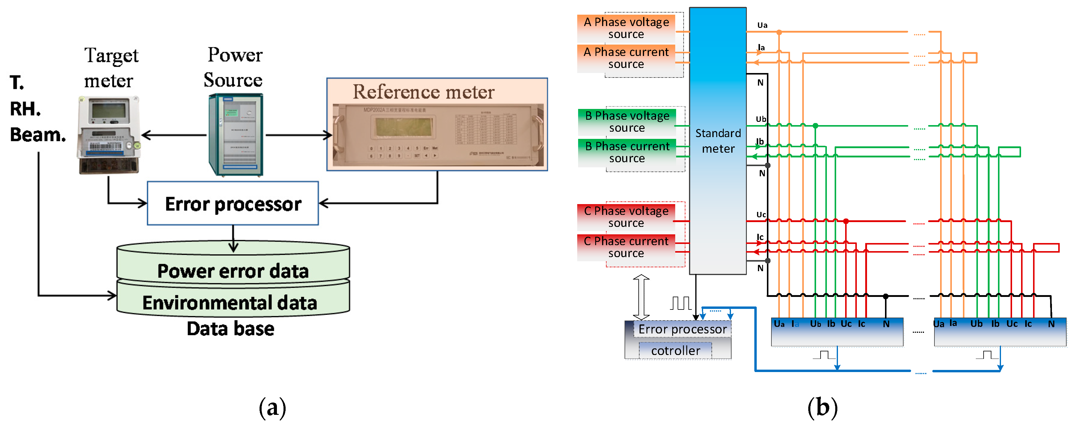
2.1. The Schematic of On-Site Operation for SEMs

All the target SEMs were installed in an uncontrolled room exposed to the natural environment, and the reference meter was installed in a temperature-controlled room at around 23 °C. A power source was employed to imitate various loadings and was connected to the target meters and the reference meter. Electricity energy was measured by both target meters and the reference meter; then the measurement error was computed in the error processor and was saved to the database every four hours. Temperature and humidity were also monitored, and the environmental data were also saved to the database. The diagram of on-site operation of SEMs is presented in Figure 1.

The electricity meters underwent testing at currents of I_max, I_b, 0.5I_b, 0.1I_b, and 0.05I_b, and power coefficients of 0.5L, 1.0, and 0.8C. I_max and I_b are the max current and basic current, L denotes inductive load, and C denotes capacitive load. The testing electrical conditions are shown in

Table 1. Electricity meter testing electrical conditions.

No.	Current	Power Coefficient	No.	Current	Power Coefficient
1	$I_{\max }$	1	8	$0.5I_b$	0.8C
2	$I_{\max }$	0.8C	9	$0.5I_b$	0.5L
3	$I_{\max }$	0.5L	10	$0.1I_b$	1
4	$I_b$	1	11	$0.1I_b$	0.8C
5	$I_b$	0.8C	12	$0.1I_b$	0.5L
6	$I_b$	0.5L	13	$0.05I_b$	1
7	$0.5I_b$	1

.

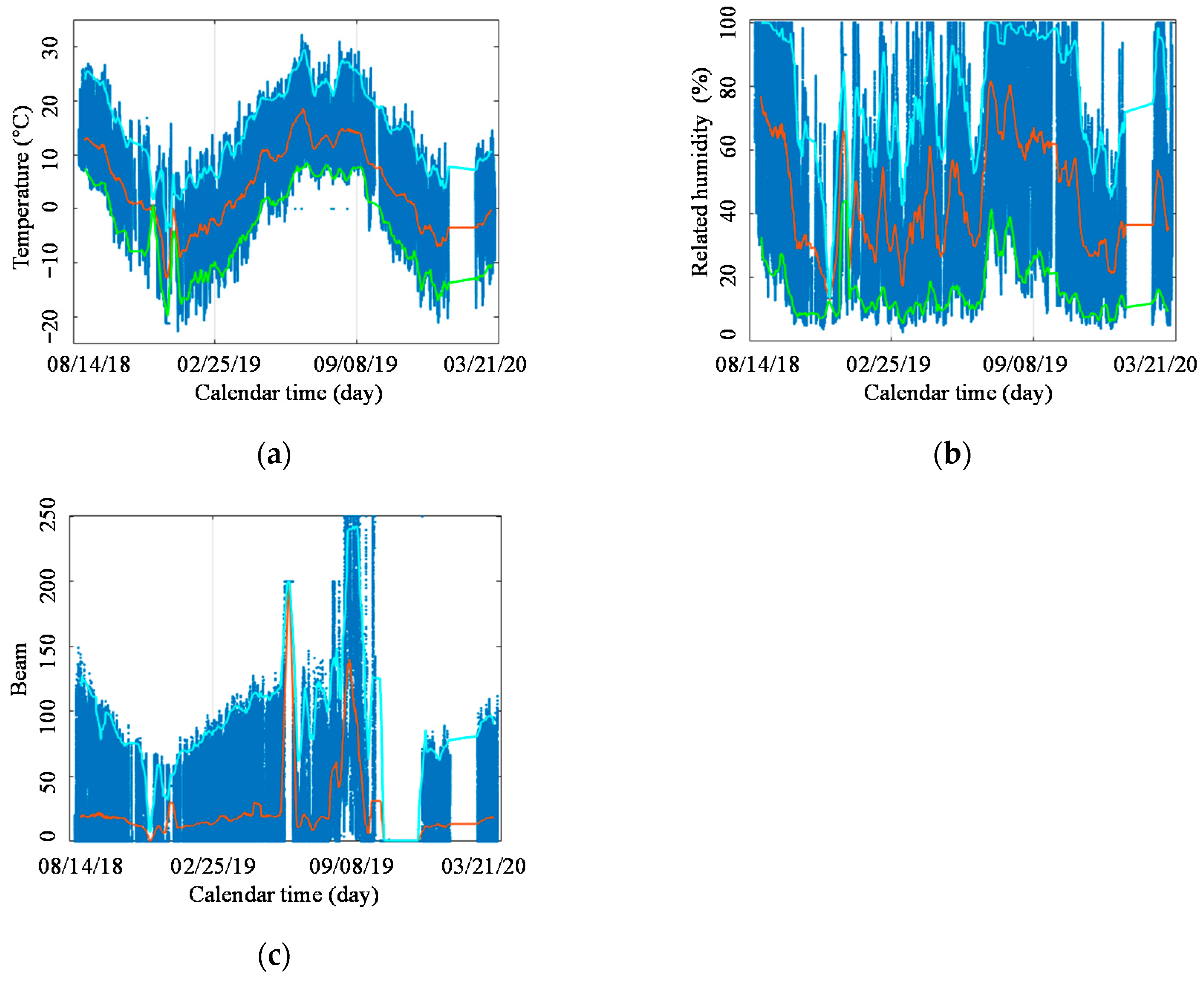
2.2. Environmental Data

Temperature, humidity, and radiation at the testing site from August 2018 to March 2020 were monitored and are shown in Figure 2. The red, blue, and green curves are the mean value curve, upper and lower envelopment lines, respectively. Temperature sinusoidally fluctuates with calendar time, and the maximum value in summer and the minimum value in winter reached 30 °C and −20 °C, respectively. The annual temperature difference reached 50 °C, as shown in Figure 2a. Humidity varies in a wide range; the maximum value and minimum value of relative humidity reached 100% and 5%, respectively, as shown in Figure 2b. Irradiation varies with seasons as shown in Figure 2c.

2.3. On-Site Measurement Error Data of SEMs

Measurement error data of 23 m under 13 testing conditions from August 2018 to December 2019 have been collected and are shown in Figure 3.

The error consistency was defined as the deviation between the measurement error and the mean value. 3σ_t was employed to describe the measurement error consistency. The smaller the value of 3σ_t was, the better the consistency of the measurement error of the smart electricity meters.

$${\sigma }_t=\frac{1}{n-1}\sqrt{{\displaystyle \sum _{i=1}^n{({\gamma }_{t,i}-{\mu }_t)}^2}},$$

(1)

where μ_t and ${\sigma }_t$ are the mean and standard deviation of the measurement error of smart electricity meters, ${\mu }_t=\frac{1}{n}{\displaystyle \sum _{i=1}^n{\gamma }_{t,i}}$, and the measurement error values at time t for n SEMs are γ_t,1, γ_t,2, …, γ_t,n.

The mean and standard deviation sinusoidally fluctuate with calendar time. Although on-site operation data reflect the real influences of environmental conditions on measurement error, the environmental factors vary with calendar time, as shown in Figure 2. As a result, it is difficult to analyze the effects of the operation conditions on measurement error of SEMs.

3. Discussion

The influences of current, power coefficient, and temperature on the measurement error of SEMs were analyzed separately, then an integrated model was developed to describe the effects of all the factors on metering error.

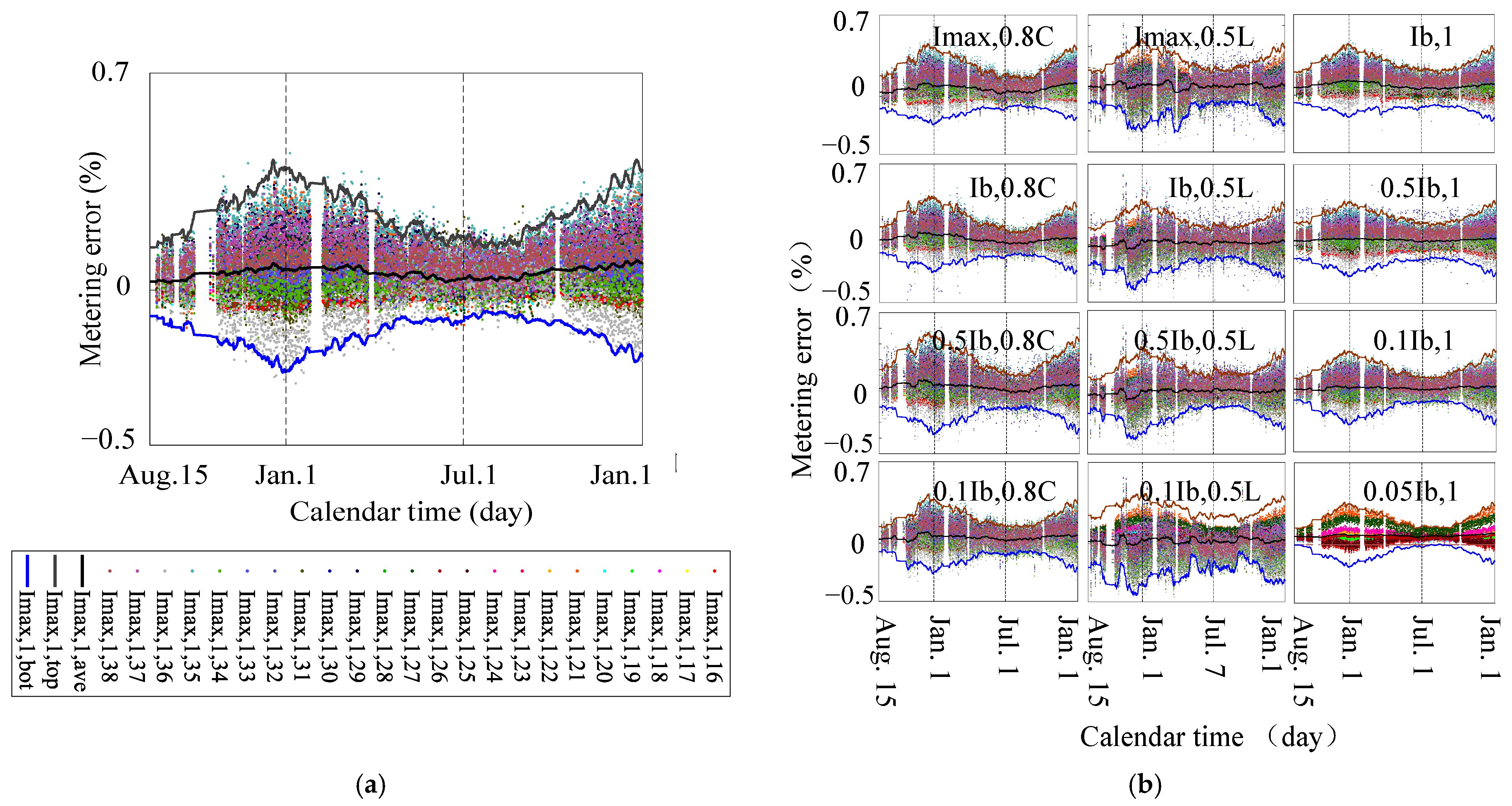
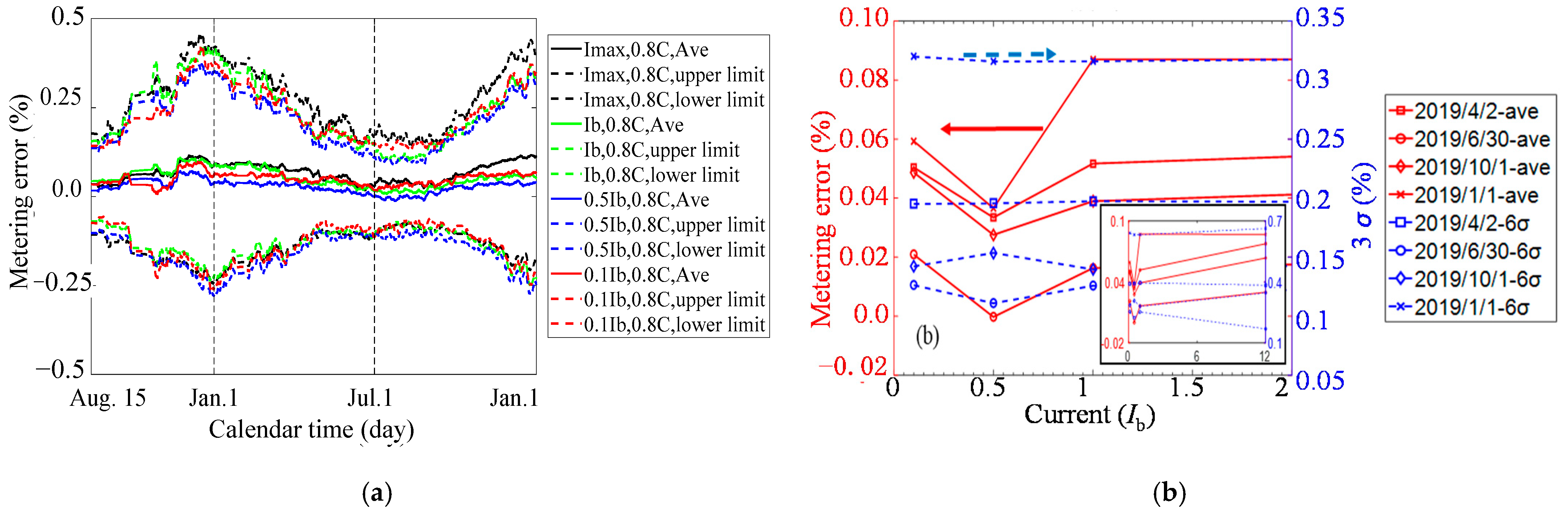
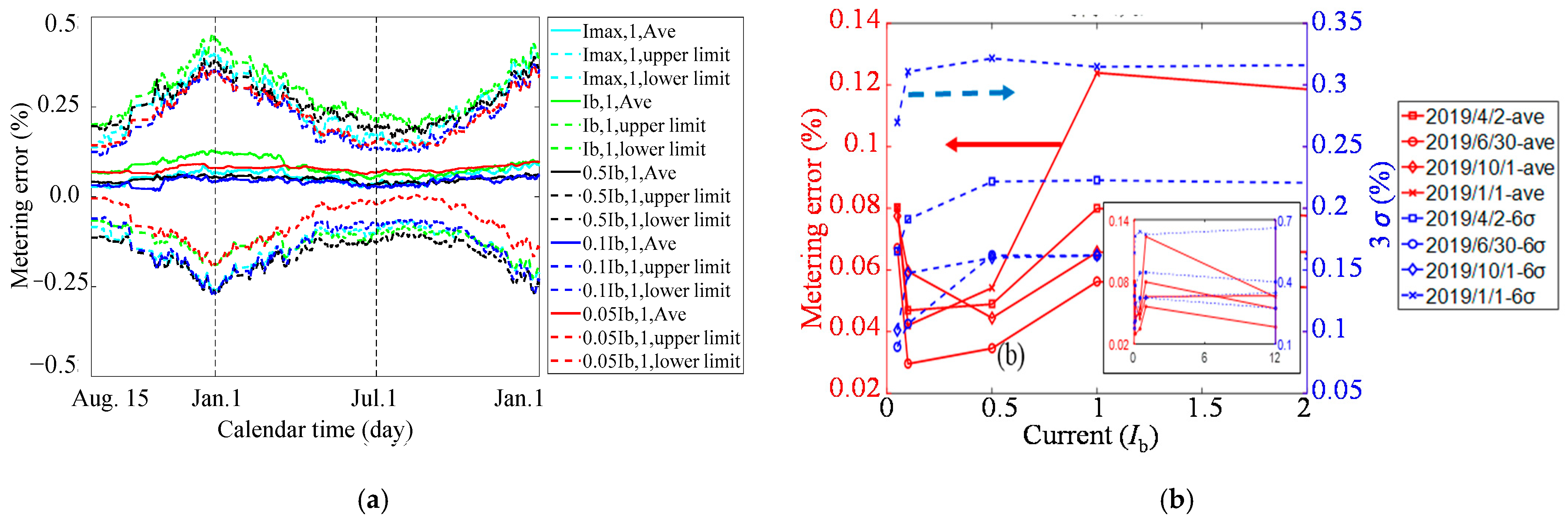
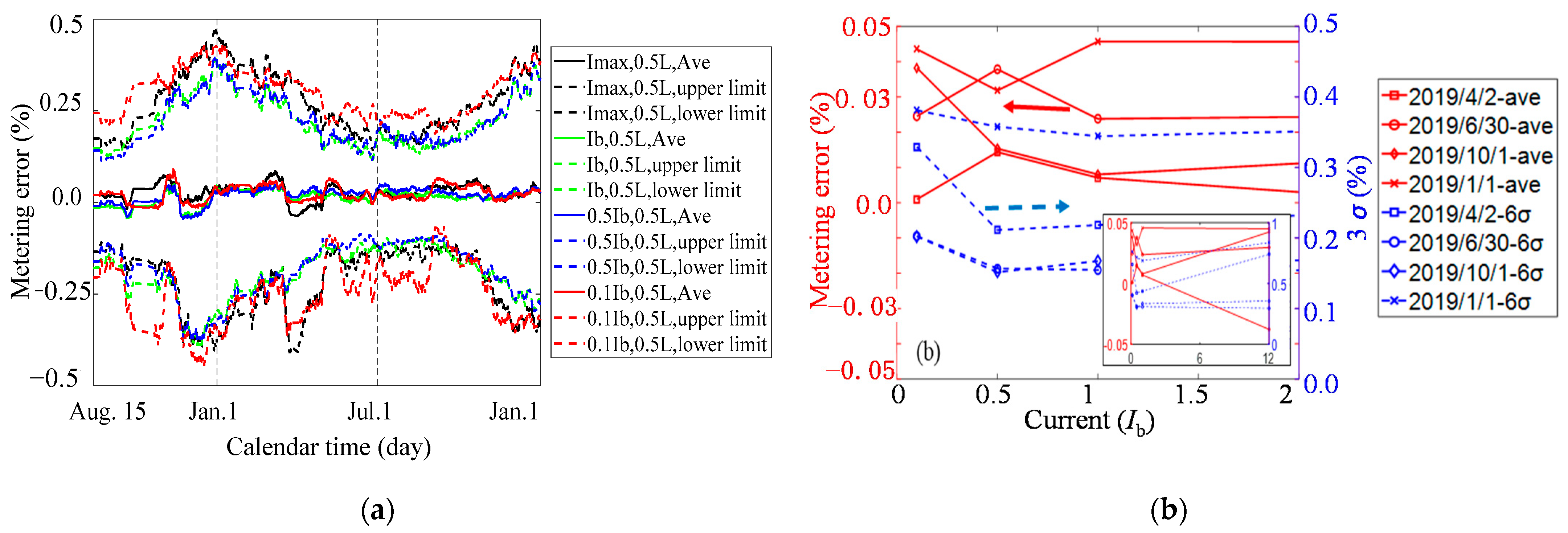
3.1. Effects of Current on Metering Error

When the power coefficient was 1.0 and the currents were $I_{\max }$, $I_b$, $0.5I_b$, $0.1I_b$ and $0.05I_b$, the mean values, upper and lower bounds of the measurement error of 23 SEMs are presented in Figure 4a. The metering errors at specific times on 1 January, 2 April, 30 June, and 1 October were selected and shown in Figure 4b. Due to the time consumed being around 30 min when the currents change from $I_{\max }$ to $0.05I_b$, the changes of environmental factors, such as temperature and humidity, could be neglected in such short time intervals. Therefore, the changes in measurement error could be considered to be caused by the alteration of current.

As shown in Figure 4b, the mean values of metering error decreased firstly and then went up with increasing current. For example, in 30 June, the measurement error declined from 0.07% at 0.05 $I_b$ to 0.03% at 0.1 $I_b$, and then raised to 0.06% at $I_b$.

The standard deviation of metering error increased fast at first and then gradually increased to a stable value. For example, on 1 October, the standard deviation increased quickly from 0.1% at 0.05 $I_b$ to 0.15% at 0.1 $I_b$, and then gradually reached 0.17% at $I_b$.

For power coefficient 0.8C and the current $I_{\max }$, $I_b$, 0.5I_b and $0.1I_b$, the mean value, upper and lower bounds of the measurement error of 23 SEMs were presented in Figure 5a. The measurement errors at specific times on 1 January, 2 April, 30 June, and 1 October were selected and are shown in Figure 5b.

As presented in Figure 5b, the mean value of measurement error decreased firstly and then increased with increasing current. For example, on 30 June, the measurement error declined from 0.05% at 0.1 $I_b$ to 0.03% at 0.5 $I_b$, and then rose to 0.05% at $I_b$. However, the standard deviation kept stable with increasing current.

For power coefficient 0.5L, the mean values and standard deviation of 23 SEMs were presented in Figure 6. The effects of currents on the mean value of the measurement error did not exhibit significant regularity, but the standard deviation declined with increasing current.

According to the variation behaviors of the mean value and the deviation of the metering error as presented in Figure 4b, Figure 5b and Figure 6b, a quadratic polynomial was employed to fit the changing trends,

γ_Ω,ψ,τ(I) = a_Ω,ψ,τ,2 I² + a_Ω,ψ,τ,1 I + a_Ω,ψ,τ,0,

(2)

where, γ_Ω,ψ,τ(I) is the function of mean value and deviation function changing with current I, a_Ω,ψ,τ,2, a_Ω,ψ,τ,1 and a_Ω,ψ,τ,0 are parameters, ψ denotes power coefficients 1.0, 0.8, and 0.5L, and τ = 1, 2, 3 denotes the specific times of 1 January, 2 April, 30 June, the parameters were computed with the help of Matlab and were presented in

Table 2. Parameter estimates for measurement error/current model.

Ω	ψ	τ	aΩ,ψ,τ,2	aΩ,ψ,τ,1	aΩ,ψ,τ,0	R2
Ω = 0, Mean	1.0	1	0.1898	−0.1367	0.0716	0.8600
		2	0.1233	−0.1154	0.0727	0.5964
		3	0.1039	−0.1039	0.0570	0.4012
	0.8C	1	0.1751	−0.1682	0.0737	1.0000
		2	0.0878	−0.0951	0.0590	1.0000
		3	0.0955	−0.1101	0.0309	1.0000
	0.5L	1	0.0635	−0.0675	0.0496	1.0000
		2	−0.0533	0.0655	−0.0051	1.0000
		3	−0.0683	0.0743	0.0178	1.0000
Ω = 1, 3σ	1.0	1	−0.1175	0.1535	0.2778	0.6302
		2	−0.1201	0.1776	0.1648	0.9273
		3	−0.1703	0.2527	0.0789	0.9940
	0.8C	1	0.0120	−0.0176	0.3215	1.0000
		2	0.0028	−0.0005	0.1950	1.0000
		3	0.0754	−0.0835	0.1339	1.0000
	0.5L	1	0.0347	−0.0789	0.3885	1.0000
		2	0.3434	−0.5009	0.3758	1.0000
		3	0.1229	−0.1887	0.2203	1.0000

.

In a summary, the mean values of measurement error decreased first and then grew with increasing current when the power coefficients were 1.0 and 0.8C, but when the power coefficient was 0.5L, the mean value of metering error did not present obvious regularity. In terms of standard deviation, the standard deviation exhibited increasing, stable, and decreasing trends with increasing current when the power coefficients were 1.0, 0.8C and 0.5L, respectively.

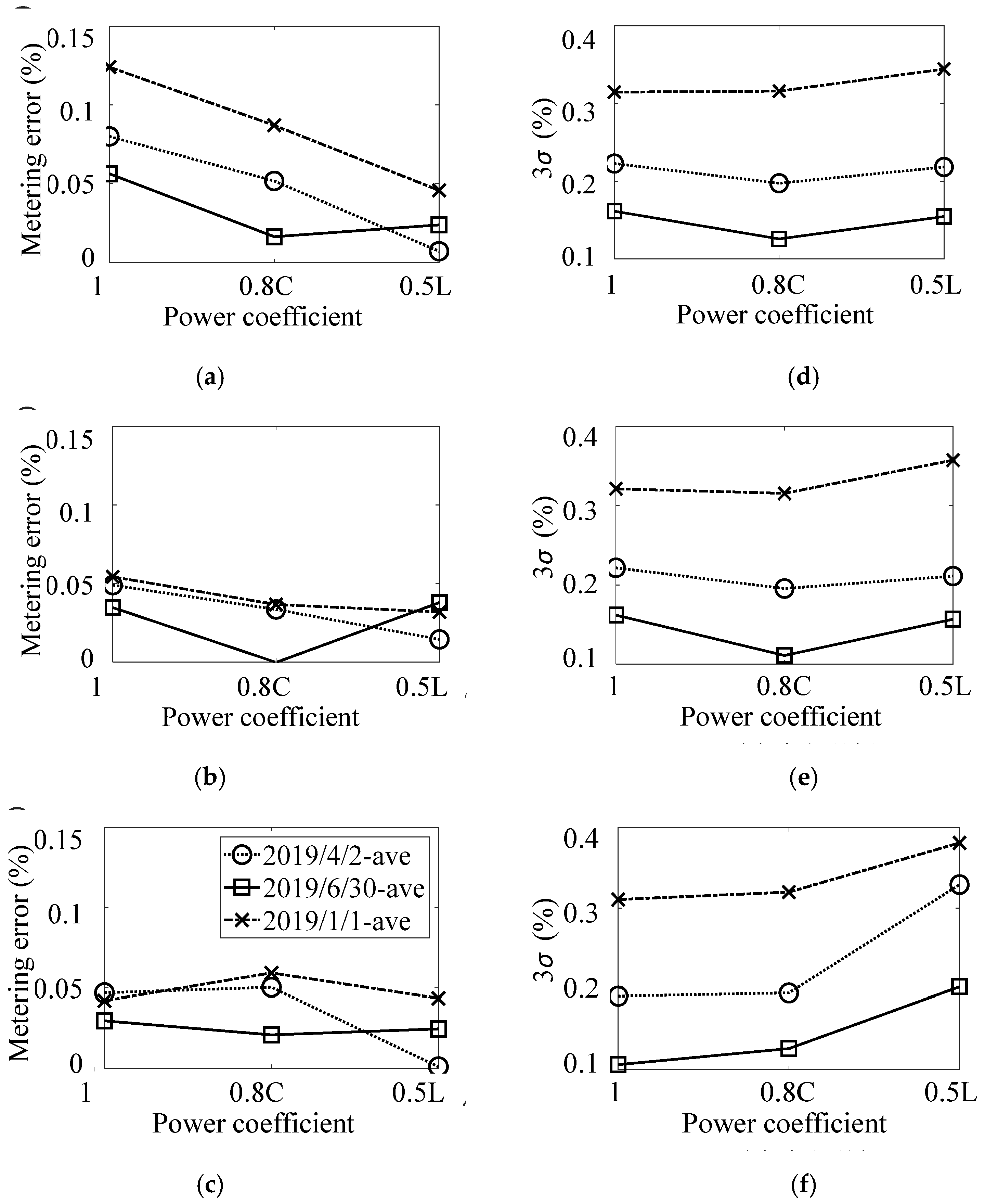
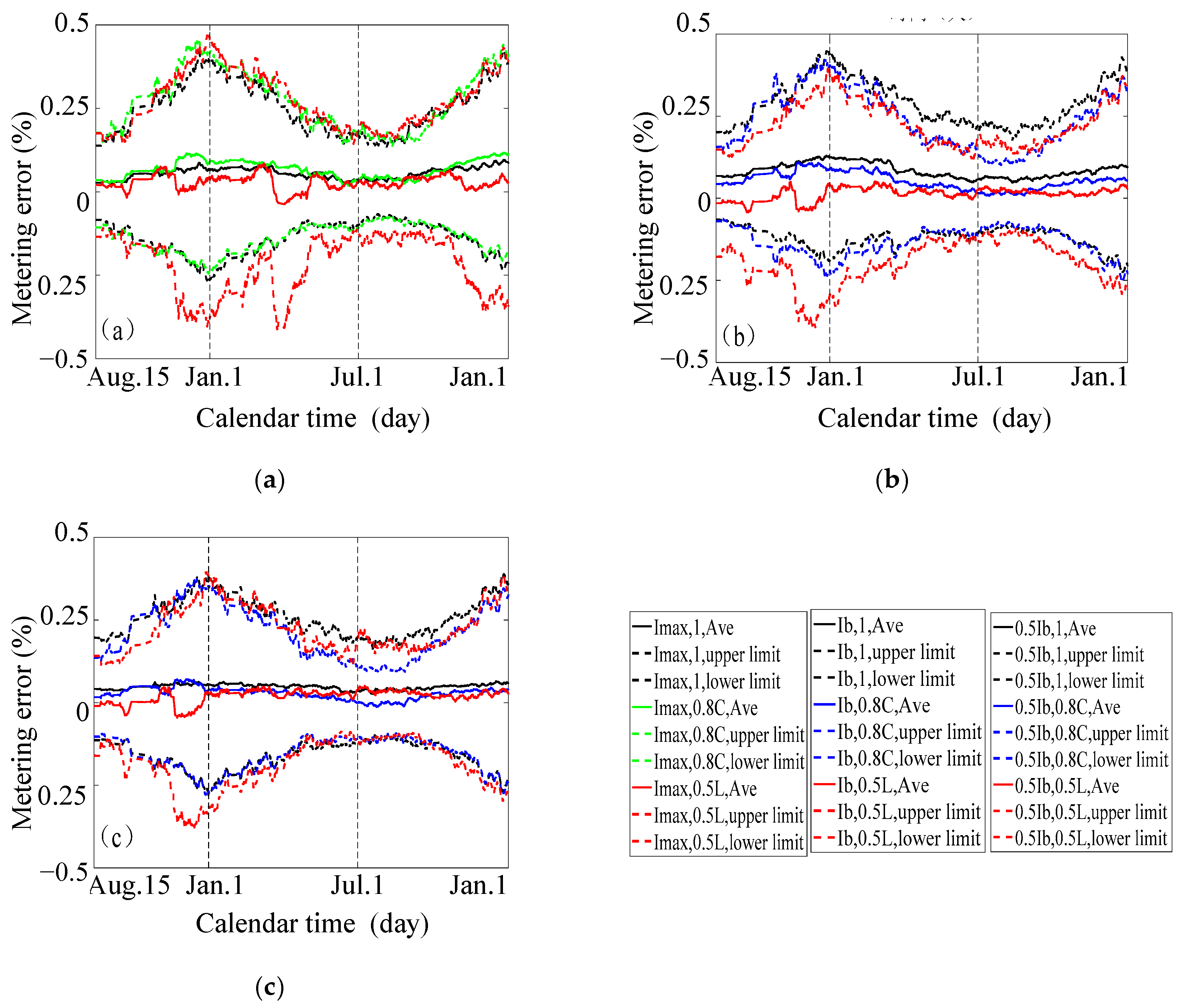
3.2. Effects of Power Coefficient on Metering Error

The mean value, upper and lower curves of metering error at currents $I_{\max }$, $I_b$ and 0.5 $I_b$ are presented in Figure 7a–c, respectively.

As shown in Figure 7, the mean value, upper and lower bounds sinusoidally fluctuated with calendar time both for power coefficients 1.0 and 0.8C. For example, the minimum and maximum of mean values were 0.0% and 0.12% and the fluctuant center was 0.06%. However, the metering error was disturbed more significantly under power coefficient 0.5L than under 1.0 and 0.8C. The mean value and standard deviation were computed at three specific times and were plotted in Figure 8.

As shown in Figure 8a–c, the mean value exhibited a declining trend when the power coefficient changed from 1.0 to 0.8C and then to 0.5L. The maximum alteration of the mean value reached 0.07% at current I_b, whereas the maximum change of mean value at current 0.5 I_b and 0.1 I_b was around 0.03% and less than the value at current I_b. However, the standard deviation of the metering error presented an increased trend when the power coefficient changed from 1.0 to 0.8C and then to 0.5L. When the current was 0.1 I_b, the maximum change of 3σ changed significantly by about 0.12%, but it varied slightly around 0.04% when the currents were I_b and 0.5 I_b.

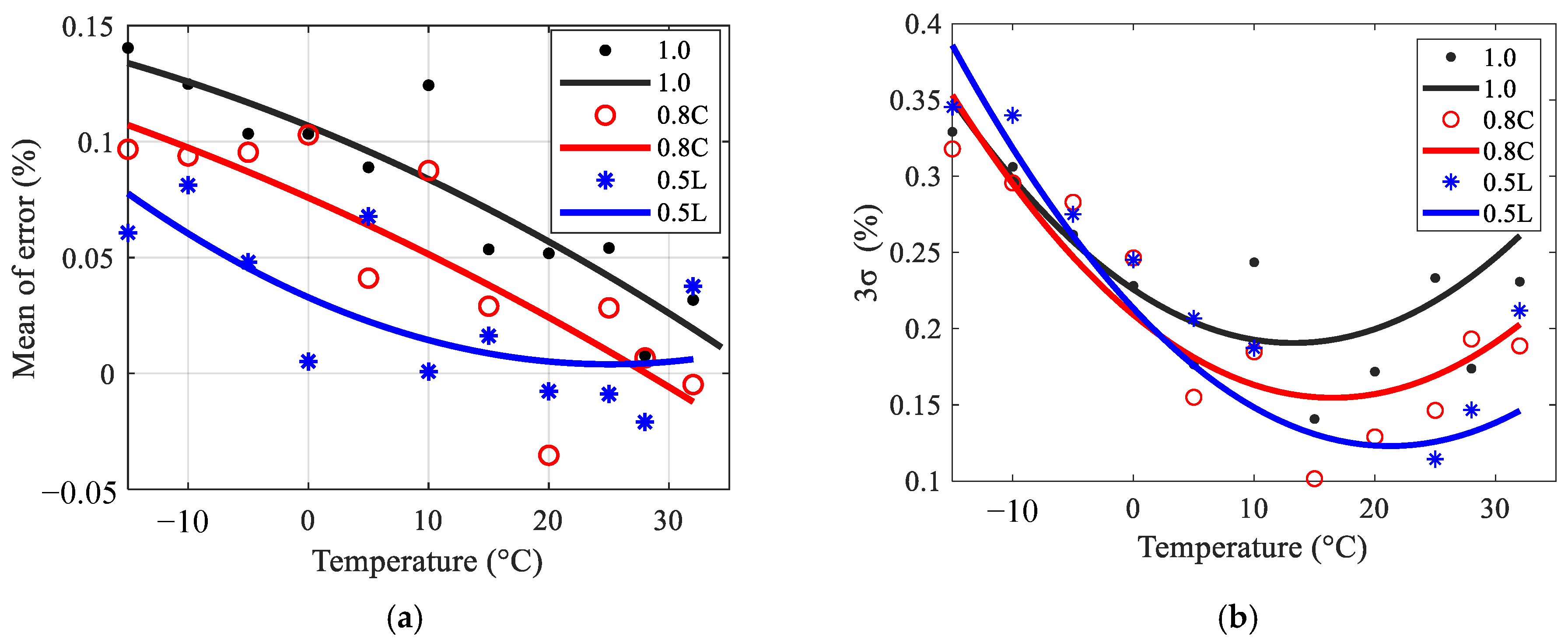
3.3. Effects of Temperature on Metering Error

Since the designed lifespan of SEMs is more than 10 years, the effects of performance degradation in 6 months on the measurement error could be neglected. Therefore, the changes of the measurement error of SEMs could be considered to be due to the changes in temperature. The measurement error at temperatures of −20, −15(5), 25, 28, 32 °C and under current I_b from 1 January 2019 to 30 June 2019 were selected and are presented in Figure 9.

As a nonlinear trend was exhibited between metering error and temperature, a quadratic polynomial was employed to fit the changing trends:

γ_Ω(T) = p_Ω,ψ,2T² + p_Ω,ψ,1 T + p_Ω,ψ,0,

(3)

where γ_Ω(T) is the function of the mean value and the deviation function changing with temperature T; p_Ω,ψ,2, p_Ω,ψ,1, p_Ω,ψ,0 are parameters, which can be computed with the help of Matlab and are listed in

Table 3. Parameter estimates for measurement error/temperature model.

Ω	ψ	pΩ,ψ,2	pΩ,ψ,1	pΩ,ψ,0	SSE	R2
Ω = 0, Mean	1.0	−1.9780 × 10−5	−0.0021	0.1068	0.0032	0.8291
	0.8C	−1.4090 × 10−5	−0.0023	0.0758	0.0068	0.7098
	0.5L	4.5830 × 10−5	−0.0023	0.0328	0.0057	0.5346
Ω = 1, 3σ	1.0	0.0002	−0.0053	0.2257	0.0084	0.7523
	0.8C	0.0002	−0.0066	0.2091	0.0086	0.8345
	0.5L	0.0002	−0.0085	0.2133	0.0160	0.8234

. The fitting curves are also presented in Figure 9.

As shown in Figure 9a, the mean value of the measurement error was inversely proportional to the temperature. For example, the mean value declined from about 0.14% at −15 °C to around 0.02% at 32 °C when the current was I_b and the power coefficient was 1.0. The results were consistent with the existing research. We also paid attention to the evolution of metering error under the other power coefficients. When the power coefficient was 0.8C, the mean value reduced from around 0.12% at −15 °C to 0.03% at 15 °C, and then to −0.02% at 32 °C. As for power coefficient 0.5L, the mean value fluctuated between −0.05% and 0.1%. However, the standard deviation exhibited a declining trend in [−15 °C, 15 °C], whereas it presented a rising trend in [15 °C, 32 °C] as shown in Figure 9b. For example, 3σ decreased from about 0.40% at −15 °C to around 0.1% at 15 °C and then increased to about 0.15% at 32 °C. The quadratic polynomial presented a good fitting result, which could be further employed to model the effects of both current and temperature.

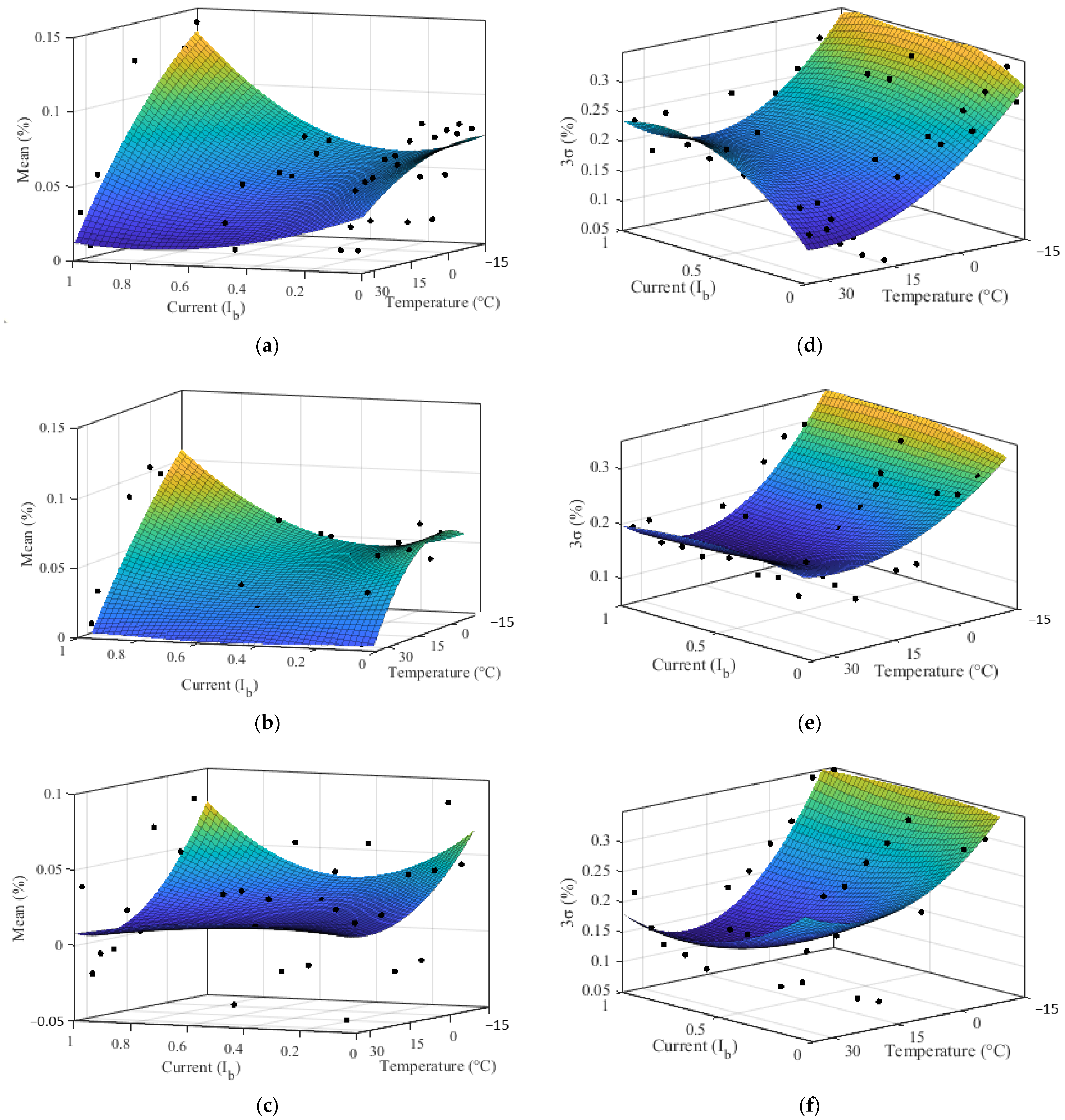
3.4. Integrated Model of Metering Error under Current and Teperature

The mean values and standard deviation of metering error under all power coefficients and currents are listed in

Table 4. Mean values of metering error under different temperatures.

Power Coefficient	Current	Mean Values of Metering Error (%)
		−15 °C	−10 °C	−5 °C	0 °C	5 °C	10 °C	15 °C	20 °C	25 °C	28 °C	32 °C
1	Ib	0.1404	0.1248	0.1034	0.1033	0.0889	0.1243	0.0535	0.0518	0.0541	0.0077	0.0317
	0.5Ib	0.0620	0.0671	0.0604	0.0739	0.0490	0.0536	0.0278	0.0188	0.0518	0.0092	0.0287
	0.1Ib	0.0731	0.0477	0.0198	0.0501	0.0219	0.0683	0.0495	0.0287	0.0107	0.0280	0.0140
	0.05Ib	0.0771	0.0821	0.0799	0.0774	0.0884	0.0785	0.0649	0.0704	0.0598	0.0583	0.0542
0.8C	Ib	0.0967	0.0938	0.0954	0.1029	0.0411	0.0875	0.0290	−0.0353	0.0283	0.0067	−0.0048
	0.5Ib	0.0501	0.0548	0.0343	0.0342	0.0153	0.0757	0.0162	0.0182	−0.0216	0.0394	−0.0057
	0.1Ib	0.0559	0.0592	0.0435	0.0712	0.0551	0.0634	−0.0194	0.0594	0.0359	0.0007	−0.0268
0.5L	Ib	0.0607	0.0812	0.0480	0.0052	0.0677	0.0008	0.0162	−0.0077	−0.0089	−0.0210	0.0376
	0.5Ib	0.0295	0.0370	0.0200	−0.0213	0.0618	−0.0218	0.0277	0.0112	0.0364	−0.0373	0.0369
	0.1Ib	0.0435	0.0861	0.0429	−0.0146	0.0437	−0.0185	0.0205	0.0695	0.0186	−0.0442	0.0301

and

Table 5. 3σ of metering error under different temperatures.

Power Coefficient	Current	3σ of Metering Error (%)
		−15 °C	−10 °C	−5 °C	0 °C	5 °C	10 °C	15 °C	20 °C	25 °C	28 °C	32 °C
1	Ib	0.3291	0.3061	0.2616	0.2281	0.1765	0.2435	0.1407	0.1718	0.2332	0.1738	0.2308
	0.5Ib	0.3259	0.3213	0.2896	0.3060	0.1876	0.1923	0.1599	0.1144	0.2460	0.1786	0.2279
	0.1Ib	0.3329	0.2973	0.2736	0.2249	0.1722	0.1850	0.2218	0.0989	0.1361	0.1680	0.1663
	0.05Ib	0.2777	0.2616	0.2439	0.2018	0.2499	0.1455	0.0569	0.0730	0.0994	0.1283	0.1256
0.8C	Ib	0.3179	0.2956	0.2829	0.2464	0.1550	0.1848	0.1016	0.1290	0.1464	0.1932	0.1887
	0.5Ib	0.3198	0.3164	0.2672	0.2141	0.1835	0.2348	0.0807	0.1239	0.1380	0.2521	0.1826
	0.1Ib	0.3193	0.2916	0.2688	0.2810	0.1604	0.1592	0.3250	0.1252	0.1605	0.1835	0.2166
0.5L	Ib	0.3453	0.3400	0.2750	0.2451	0.2068	0.1873	0.0590	0.0900	0.1144	0.1466	0.2118
	0.5Ib	0.3226	0.3109	0.2793	0.2544	0.2226	0.2143	0.0783	0.0789	0.1556	0.1776	0.1915
	0.1Ib	0.3546	0.3122	0.3021	0.3557	0.2131	0.3593	0.0799	0.0925	0.2031	0.3854	0.1881

.

The mean value and standard deviation of the metering error presented a nonlinear trend with increasing temperature as shown in Figure 9a,b and with increasing current as shown in Figure 6b and Figure 7b, respectively. So, a binary quadratic polynomial was employed to fit the joint influences of current and temperature on the mean and standard deviation of the measurement error. The model was written as:

$$\gamma \mathsf{\Omega }\left(T,I\right)={\left[\begin{array}{c}{I}^2\\ I\\ 1\end{array}\right]}^{\prime }\left[\begin{array}{ccc}{w}_{c,\mathsf{\Omega }}& w_{b,\mathsf{\Omega }}& w_{a,\mathsf{\Omega }}\\ u_{c,\mathsf{\Omega }}& u_{b,\mathsf{\Omega }}& u_{a,\mathsf{\Omega }}\\ v_{c,\mathsf{\Omega }}& v_{b,\mathsf{\Omega }}& v_{a,\mathsf{\Omega }}\end{array}\right]\left[\begin{array}{c}{T}^2\\ T\\ 1\end{array}\right],$$

(4)

where γ_Ω(T,I) is the mean function and the standard deviation function about the random variable of temperature T and current I when Ω = 0 and Ω = 1. The model parameters are w_a,Ω, u_a,Ω, v_a,Ω, w_b,Ω, u_b,Ω, v_b,Ω, w_c,Ω, u_c,Ω, v_c,Ω. The estimates of the model parameters were computed using Matlab tools and are presented in

Table 6. Model parameter estimates.

Ω	Parameters	Power Coefficient
		1.0	0.8C	0.5L
Ω = 0, Mean	wa,0	0.1450	0.1284	0.0747
	ua,0	−0.1095	−0.1214	−0.0787
	va,0	0.0719	0.0688	0.0368
	wb,0	−0.0010	−0.0024	−0.0057
	ub,0	−0.0007	0.0006	0.0054
	vb,0	−0.0003	−0.0005	−0.0020
	wc,0	−5.4070 × 10−5	−0.0001	7.5650 × 10−5
	uc,0	5.2410 × 10−5	0.0002	−6.7290 × 10−5
	vc,0	−1.8450 × 10−5	−6.9960 × 10−5	3.7470 × 10−5
	SSE	0.0134	0.0176	0.0269
	R-square	0.6863	0.6161	0.2803
Ω = 1, 3σ	wa,1	−0.1093	0.0631	0.1031
	ua,1	0.1346	−0.1017	−0.1729
	va,1	0.1999	0.2477	0.2813
	wb,1	0.0015	0.0051	0.0001
	ub,1	−0.0010	−0.0081	−0.0037
	vb,1	−0.0058	−0.0037	−0.0049
	wc,1	−0.0001	−0.0003	7.4560 × 10−5
	uc,1	0.0002	0.0004	1.1790 × 10−5
	vc,1	8.9980 × 10−5	6.0890 × 10−5	0.0001
	SSE	0.0534	0.0584	0.1234
	R-square	0.7646	0.6514	0.5888

, the fitting results are plotted in Figure 10.

As shown in Figure 10, the metering error was severely affected by current and environmental temperature. For power coefficient 1.0, as presented in Figure 10a, the effects of temperature on metering error were more severe under the large current (I_b) than under the small current (0.1 I_b). A higher temperature and a larger current resulted in a higher metering error of SEMs. For power coefficient 0.8C, as shown in Figure 10b, the current slightly influenced the metering error at high temperatures, such as 30 °C, but when the temperature was low, such as −15 °C, the metering error reduced first and then rose with increasing current. However, whether at a low or a high current, the effects of temperature on metering error exhibited a rising trend with decreasing temperature. In addition, the metering error exhibited an increasing trend when the temperature was decreasing, and the current became larger. As for the power coefficient 0.5L, the influences of temperature and current presented a disordered trend as presented in Figure 10c, and the goodness of fitting was not good due to a low R-square of 0.2803 as listed in Table 6.

In terms of the error consistency, the decreasing temperature, from 32 °C to about 15 °C, generated a slight decrease in the standard deviation, but the decreasing temperature, from 15 °C to around −15 °C, resulted in a significant increment at the power coefficients 1.0, 0.8C, and 0.5L, as shown in Figure 10d–f, respectively. However, the current generated different effects on the standard deviation under different power coefficients. The standard deviation exhibited an increasing trend, a stable trend, and a decreasing trend with increasing current under power coefficients 1.0, 0.8C, and 0.5L, respectively.

4. Conclusions

An integrated model was developed to describe the joint effects of both temperature and current on the metering error and consistency of SEMs based on a binary quadratic polynomial. The results show that a lower temperature and a larger current result in a higher metering error of SEMs. Temperature significantly affects metering error—low temperatures (−15 °C) generate the highest measuring error, and high temperatures (32 °C) produce the smallest measurement error, which is consistent with existing studies. Moreover, temperature determines the effects of current on metering error since the current generates more severe influences on metering error under low temperatures than under high temperatures.

In addition, the effects of temperature on standard deviation are different from the influences of current on standard deviation. The standard deviation declines with decreasing temperature from [32 °C, 15 °C], but increases from [15 °C, −15 °C]. The effects of current on standard deviation depend on the power coefficient, and exhibit a decreasing trend, a stable trend, and an increasing trend with decreasing current under power coefficients 1.0, 0.8C, and 0.5L, respectively.

For the effects of power coefficients on the metering error of SEMs, the metering error exhibited disordered behaviors under power coefficient 0.5L compared to 1.0 and 0.8C. If we investigate how the power coefficient will affect the influences of temperature and current on metering error, the effects of current on measurement error are determined by the power coefficient, whereas the influences of temperature on the measuring error are slightly disturbed by the power coefficient.

Why temperature, current, and power coefficient affect the metering error of SEMs needs to be further studied.

References

1. Yao, L.; Zhang, J.M.; Hu, Y.J. Study on running reliability data processing method for smart electrical energy meters. Bull. Sci. Technol. 2018, 34, 125–129. [Google Scholar]
2. Yang, Z.; Diao, D.C.; Lu, H.J.; Sun, Q.X.; Wu, S. Review and prospect of research on reliability test method of electric energy meters. Electr. Meas. Instrum. 2020, 57, 17–25. [Google Scholar]
3. Bai, Y.D. The Stability Research of Electric Energy Meter Based on Accelerated Degradation Test. Master’s Thesis, National University of Defense Technology, Changsha, China, 2016. [Google Scholar]
4. Yang, Z.; Chen, Y.X.; Li, Y.F.; Zio, E.; Kang, R. Smart Electricity Meter Reliability Prediction based on Accelerated Degradation Testing and Modeling. Int. J. Electr. Power Energy Syst. 2014, 56, 209–219. [Google Scholar] [CrossRef] [Green Version]
5. Plenz, M.; Dong, C.; Grumm, F.; Meyer, M.F.; Schumann, M.; McCulloch, M.; Jia, H.; Schulz, D. Framework Integrating Lossy Compression and Perturbation for the Case of Smart Meter Privacy. Electronics 2020, 9, 465. [Google Scholar] [CrossRef] [Green Version]
6. Apse-Apsitis, P.; Vitols, K.; Grinfogels, E.; Senfelds, A.; Avotins, A. Electricity meter sensitivity and precision measurements and research on influencing factors for the meter measurements. IEEE Electromagn. Compat. Mag. 2018, 7, 48–52. [Google Scholar] [CrossRef]
7. Wang, X.W.; Wang, J.; Yuan, R.M.; Jiang, Z.Y. Orthogonal pseudo-random measurement dynamic test signal modeling and dynamic error indirect test method of likelihood function for electricity meter. Proc. CSEE 2019, 39, 6686–6699. [Google Scholar] [CrossRef]
8. Wang, Y.; Chen, Q.; Hong, T.; Kang, C. Review of smart meter data analytics: Applications, methodologies, and challenges. IEEE Trans. Smart Grid 2019, 10, 3125–3148. [Google Scholar] [CrossRef] [Green Version]
9. Alahakoon, D.; Yu, X. Smart electricity meter data intelligence for future energy systems: A survey. IEEE Trans. Ind. Inform. 2016, 12, 425–436. [Google Scholar] [CrossRef]
10. Cheng, X.Q.; Yu, M.Q.; Liu, M.H.; Huang, R.; Xie, L.J.; Tan, H.B. Research on comprehensive performance evaluation method of smart energy meter. In Proceedings of the 2018 3rd International Conference on Mechanical Control and Computer Engineering (ICMCCE), Harbin, China, 8–10 December 2018; pp. 450–455. [Google Scholar]
11. Jiao, Y.; Li, H.B.; Hu, C.; Zhang, Z.; Zhang, C.J. Data-driven evaluation for error states of standard electricity meters on automatic verification assembly line. IEEE Trans. Ind. Inform. 2019, 15, 4999–5006. [Google Scholar] [CrossRef]
12. Yin, X.; Lu, Y.B.; Gong, Y.; Han, D.; Sun, Y.; Liu, H.Y.; Liang, Y.H. The error model of the smart meter under influence of temperature. Electr. Meas. Instrum. 2017, 54, 85–88. [Google Scholar]
13. Xu, Q.; Cheng, H.M.; Cai, Q.X.; Ji, F.; Li, J.; Gao, Y.X.; Li, X.R. Study on the influence of environmental factors on the basic error of single-phase electricity meters. Electr. Meas. Instrum. 2020, 57, 119–125. [Google Scholar]
14. Zheng, J.; Chen, L.; Yuan, W.; Dong, S.F.; Wu, Y.H.; Zhang, L.P. Study on error of meter with environmental factors under high altitude typical environment. Electr. Meas. Instrum. 2019, 56, 135–140. [Google Scholar]
15. Kong, X.; Zhang, X.; Li, G.; Dong, D.; Li, Y. An estimation method of smart meter errors based on DREM and DRLS. Energy 2020, 204, 117774. [Google Scholar] [CrossRef]
16. Edgars, G.; Peteris, A.A.; Senfelds, A.; Avotins, A.; Porins, R. Electrical power measurement method comparison using statistical analysis. In Proceedings of the 2018 IEEE 59th International Scientific Conference on Power and Electrical Engineering of Riga Technical University (RTUCON), Riga, Latvia, 12–14 November 2018; pp. 1–4. [Google Scholar]
17. Lu, M.D. Analysis and Optimization of Metering Accuracy Consistency of Smart Power Meter Considering Temperature Effect. Master’s Thesis, Harbin Ind. Univ., Harbin, China, 2018. [Google Scholar]
18. Yuan, R.M.; Lv, Y.G.; Jiang, Z.Y.; Li, W.W.; Ye, X.R.; Yang, H.Z.; Zhou, S.G.; Liu, L.; Xie, X.Y.; Zhai, G.F. Analysis and optimization design of intelligent meter measurement error consistency. Electr. Energy Manag. Technol. 2017, 17, 26–30. [Google Scholar]
19. Cai, H.; Chen, H.; Ye, X.; Zhang, X.; Wen, H.; Li, J.; Guo, Q. An on-line state evaluation method of smart meters based on information fusion. IEEE Access 2019, 7, 163665–163676. [Google Scholar] [CrossRef]
20. Avancini, D.B.; Rodrigues, J.J.P.C.; Martins, S.G.B.; Rabêlo, R.A.L.; Al-Muhtadi, J.; Solic, P. Energy meters evolution in smart grids: A review. J. Clean. Prod. 2019, 217, 702–715. [Google Scholar] [CrossRef]
21. Kong, X.; Ma, Y.; Zhao, X.; Li, Y.; Teng, Y. A recursive least squares method with double-parameter for online estimation of electric meter errors. Energies 2019, 12, 805. [Google Scholar] [CrossRef] [Green Version]
22. Abate, F.; Carratù, M.; Liguori, C.; Paciello, V. A low-cost smart power meter for IoT. Measurement 2019, 136, 59–66. [Google Scholar] [CrossRef]
23. Kemal, M.; Sanchez, R.; Olsen, R.; Iov, F.; Schwefel, H.P. On the trade-off between timeliness and accuracy for low voltage distribution system grid monitoring utilizing smart meter data. Int. J. Electr. Power Energy Syst. 2020, 121, 106090. [Google Scholar] [CrossRef]
24. Liu, X.L.; Cui, W.J.; Li, J.M. Electric Energy Meter Online Detection Method. WIPO Patent Application WO/2012/174693, 27 December 2012. [Google Scholar]
25. Nakutis, Ž.; Saunoris, M.; Ramanauskas, R.; Daunoras, V.; Lukočius, R.; Marčiulionis, P. A method for remote estimation of wattmeter’s adjustment gain. IEEE Trans. Instrum. Meas. 2018, 68, 713–721. [Google Scholar] [CrossRef]
26. Nakutis, Ž.; Kaškonas, P.; Saunoris, M.; Daunoras, V.; Jurčević, M. A framework for remote in-service metrological surveillance of energy meters. Measurement 2021, 168, 108438. [Google Scholar] [CrossRef]
Figure 1. Diagram of on-site operation of smart electricity meters. (a) on-site operation process; (b) scheme of the experimental set-up.
Applsci 11 11457 g001
Figure 2. Environmental data. (a) Temperature vs. time; (b) Humidity vs. time; (c) Irradiation vs. time.
Applsci 11 11457 g002
Figure 3. Metering error of 23 electricity meters under all test conditions. (a) Error data under conditions of current I max and power coefficient 1.0; (b) Error data under the remaining conditions. The black, red, and blue curves are the mean value curves, upper, and lower envelopment lines, respectively.
Applsci 11 11457 g003
Figure 4. Metering error of batch electricity meters under conditions of (power coefficient: 1.0). (a) The evolution of mean values and upper and lower bounds of metering error with calendar time; (b) The changing trends of mean value and 3σ of metering error with current.
Applsci 11 11457 g004
Figure 5. Metering error of batch electricity meters under conditions of (power coefficient: 0.8C). (a) The evolution of mean values and upper and lower bounds of metering error with calendar time; (b) The changing trends of mean value and 3σ of metering error with current.
Applsci 11 11457 g005
Figure 6. Metering error of batch electricity meters under conditions of (power coefficient: 0.5L). (a) The evolution of mean value and upper and lower bounds of metering error with calendar time; (b) The changing trends of mean value and 3σ of metering error with current.
Applsci 11 11457 g006
Figure 7. Metering error of SEMs under conditions of (ac) for current: I max , I b , and 0.5 I b , respectively.
Applsci 11 11457 g007
Figure 8. Metering error under various power coefficients, (a,d), (b,e), (c,f) for current I b , 0.5 I b and 0.1 I b .
Applsci 11 11457 g008
Figure 9. Measurement error under various levels of power coefficient, (a,b) for mean values and standard deviation, respectively.
Applsci 11 11457 g009
Figure 10. Fitting results. (a,d), (b,e), (c,f) are for power coefficients 1.0, 0.8C, and 0.5L, respectively.
Applsci 11 11457 g010