Abstract
To decrease human and economic damage owing to earthquakes, it is necessary to discover signals preceding earthquakes. We focus on the concept of “early warning signals” developed in bifurcation analysis, in which an increase in the variances of variables precedes its transition. If we can treat earthquakes as one of the transition phenomena that moves from one state to the other state, this concept is useful for detecting earthquakes before they start. We develop a covariance matrix from multi-channel time series data observed by an observatory on the seafloor and calculate the first eigenvalue and corresponding eigenstate of the matrix. By comparing the time dependence of the eigenstate to some past earthquakes, it is shown that the contribution from specific observational channels to the eigenstate increases before earthquakes, and there is a case in which the eigenvalue increases as predicted in early warning signals. This result suggests the first eigenvalue and eigenstate of multi-channel data are useful to identify signals preceding earthquakes.
1. Introduction
Determining precursor signals of earthquakes is sought as earthquakes result in considerable damage including economic loss and fatalities. If these could be determined, the damage resulting from earthquakes could be reduced by countermeasures such as stopping the use of equipment, and evacuation to a safe location. Certainly, earthquake early warnings are effective for locations away from the epicenter. On the other hand, they are unhelpful for locations near the epicenter because they warn only after earthquakes occur. Thus, preceding earthquake signals are desired. However, no conclusive method has been developed owing to the complexity of earthquakes such as a variety of crustal hardness and applied stress inhomogeneity.
There are studies determining preceding signals via defining feature quantities and analytical methods describing their behaviors. Some regard observable physical quantities as feature quantities, and adopt their change as preceding signals. Examples of such studies include those of earthquake lights [1], groundwater levels [2], earth current [3,4], very low frequencies [5], crustal deformation measured using a global positioning system [6] and ionospheric anomalies [7,8]. Other studies have extracted feature quantities from physical quantities via the use of statistical methods. The correlation between the b-value and earth tide [9] is found out by insight. Machine learning methods [10] are one trends in statical methods. There are example such as using the earth current [11] and radon monitoring [12]. Nevertheless, it cannot be said that the method to determine preceding earthquake signals is established. In the case of electro-magnetic phenomena and ionospheric anomalies, the relations between observed physical quantities and an earthquake are not direct. Earthquake lights and the change in the confined groundwater level are the consequences of a particular locality and do not have generality. Concerning the studies using machine learning, they inherently need a large amount of data and they have difficulty showing generality, i.e., independence of locality owing to data. Crustal deformation measured using the global positioning system seems to be closely related to earthquakes but it does not show clear preceding signals.
Feature quantities extracted from data that have a strong relation to earthquake activity such as velocity and acceleration on the surface of earth are a promising candidate for general preceding signals. Observational points are already established on the ground surface and observed time series data of several physical quantities are available. It is natural that these data have a direct relation to the state of the crust because of certain continuity between the observed point and epicenter. Thus, feature quantities extracted from these observed data are candidate for preceding signals if such signals exist.
If we can treat earthquakes as one of the transition phenomena from one state to the other state, the methods termed “early warning signals (EWSs)” [13], which is one of the preceding signals, are available. EWSs are methods focusing on increasing fluctuations in variables and decreasing recovery rates against disturbances when the system reaches the vicinity of the transition point. EWSs based on a covariance matrix detect preceding signals from the relation between multiple types of time series data. It adopts the first eigenvalue as a preceding signal. In addition, the EWS termed “dynamical network marker” not only constructs preceding signals but also extracts variables contributing to the transition via the use of eigenstates [14,15,16]. In the case of earthquakes, in which the process of the transition is complex, the eigenstate is expected to play an important role as a factor estimation or as preceding signals themselves.
Thus, we propose a method to detect preceding earthquake signals via a transition of the first eigenvalue and the corresponding eigenstate of the covariance matrix developed from observed data such as velocity and acceleration of the ground surface such as the EWS methods.
The rest of the paper is organized as follows. In Section 2, we introduce materials and methods. This section consists of two subsections, “Data sets and pre-processing” and “Methodology”. Next, in Section 3, we show the analysis results by the means of EWSs. Then, in Section 4, we discuss the relation between the analysis results and earthquake location. Finally, in Section 5, we summarize conclusions.
2. Materials and Methods
2.1. Data Sets and Pre-Processing
We adopt multi-channel time series data observed by the Dense Oceanfloor Network system for Earthquakes and Tsunamis (DONET) which are partly published on the website of the Japan Agency for Marine-Earth Science and Technology (JAMSTEC). DONETs were first installed offshore of Kii Peninsula (DONET1) and then installed offshore of Shikoku Island (DONET2) in Japan. They have multi-channel sensors such as seismometers, accelerometers, pressure gauges, thermometers, and inclinometers at some hundreds of meters under the ocean floor [17,18]. Thus, less artificial noise is expected. Here, we use available open data from the station termed KMDB1 in DONET1 which has published time series data on and after 1 April 2015. The KMDB1 station is at a latitude of 33.18 degrees North and a longitude of 136.3 degrees East and is 1936 m below sea level. The sampling frequencies of sensors are at least 1 Hz and at most 125 Hz. We converted the time series data from the SEED format to the ASCII format using “rdseed” (version 5.3.1), which is available to the public from the Incorporated Research Institutions for Seismology [19].
A desirable time scale for preceding signals may be at least a few minutes and at the most a few weeks. Thus, sampling at 1 Hz is enough to extract preceding signals. Time-series physical quantities are reproduced from the SEED file and RESP file provided by DONETs. The conversion coefficient at 1 Hz for each sensor is explicitly written as the represented value in the RESP file. Hence, we simply multiply the conversion coefficients by the observed value. For the channels that have a higher sampling frequency than 1 Hz, the sampling rate is reduced to 1 Hz by taking moving average.
2.2. Methodology
In reference to EWSs, we adopt the first eigenvalue and the corresponding eigenstate of the covariance matrix of the observed data as a feature quantity. To create a covariance matrix, we define a time window in which each data point is regarded as a sample for the matrix. The time dependence of the matrix is based on the feature quantities obtained by sliding the time window. We term the width of the slide a time step; the relation is shown in Figure 1.
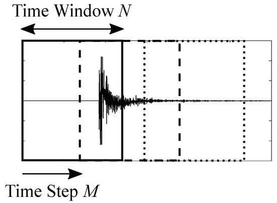
Figure 1.
Setting of time windows (solid, dashed, and dotted lines) and time steps for an observed data.
Here, we mention that the end time of the window corresponds to the present time because we can analyze only past data. Thus, we must extract preceding signals before a window includes the main shock data of an earthquake.
We extract feature quantities based on the concept of an EWS from multi-channel time series data at a 1 Hz sampling as in the following procedures.
- Prepare multi-channel time series data with the indexes of the sensor channel i () and discrete time q (). Then, set the time step width M and time window width N. Analysis of the object for the pth time step is from to .
- Define a variable that represents the fluctuation from the average of the data in the time window.
- Create normalized data with normalization constant for channel i which is the average of the absolute value of at some time window .
- Define matrix which has the element for the ith row and the jth column.
- Develop a following covariance matrix using and its transverse matrix .
- Calculate the sets of eigenvalues and eigenstate by means of the eigenvalue decomposition of . Here, we define r () as the index of the eigenvalue which has the rth largest value.
- Calculate p-dependence, i.e., the time dependence of eigenstate corresponding to the first eigenvalue .
- Compare the time dependence to earthquakes focusing on the eigenvalue and the contribution weight to the eigenstate from the original channel. The contribution weights are defined as follows:Here, is the eigenstate, and , , ⋯, are the bases that represent the original channel as used in Equation (4).
According to the EWS concept, contributions from specific channels related to a transition will increase prior to an earthquakes. Thus, we define an occupancy rate , which is a ratio of the weights of specific R channels, named , ⋯, :
In typical EWS theory, both an increase in eigenvalue and occupancy rate from specific channels is expected.
We selected three earthquakes as listed in Table 1 to be analysis objects whose waveforms were observed by DONET, and visualized location of the epicenters and the KMDB1 station of DONET observatory in Figure 2. Hereafter, we term each earthquake simply the Mie, Kumamoto, or Fukushima earthquake.

Table 1.
Earthquakes of 2016 analyzed [20].
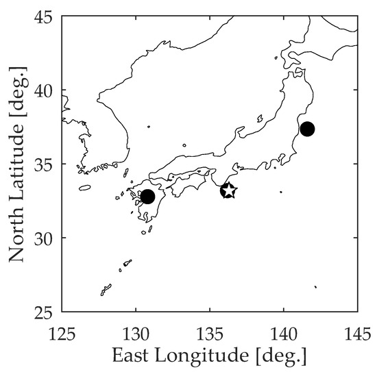
Figure 2.
Location of the epicenters and the KMDB1 station of DONET observatory. The epicenters are shown as filled circle, and the KMDB1 station is shown as a pentagram.
As listed in Table 1, the Mie earthquake occurred very near the location of the KMDB1 station and its depth was shallow at 29 km. Thus, we expect that the observed data include information regarding some changes in the crustal state. The others, Kumamoto and Fukushima earthquakes, have similar energy scales to that of the Mie earthquake at moment magnitude 7 and 6.9, but they occurred far from the station. As an example of the reproduced waveform from a SEED file, we show representative waveforms, in which the average values are subtracted from original data, from 20:00 during the day before the Mie earthquake to 0:00 during the day of the earthquake in Figure 3.
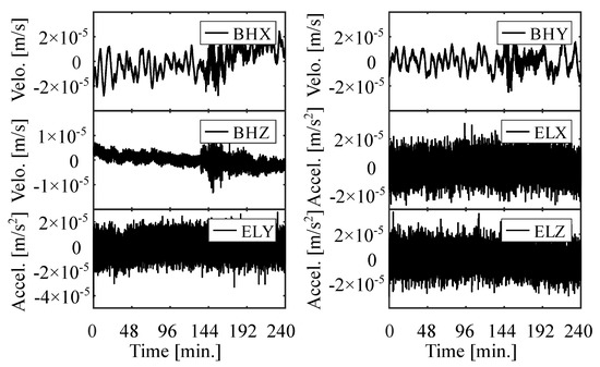
Figure 3.
Representative waveforms for the Mie earthquake. The origin of the time is 20:00 on 31 March.
Here, BHX, BHY, BHZ, ELX, ELY, and ELZ are the waveforms in the x, y, z direction of the velocity type seismometer, and x, y, z direction of the accelerometer, respectively. Since the change of the other quantities are not at the time scale for expected preceding signals, We adopt only these waveform data for EWS analysis.
We provide channel numbers 1, 2, 3, 4, 5, and 6 to BHX, BHY, BHZ, ELX, ELY, and ELZ, respectively. We adopt the channel number L, the time step width M, and the time window N as 6, 200, and 400, respectively. As we treat the sampling frequency as 1 Hz, the unit of M and N is the same with time (seconds). We set the time window N to 400, so we have 400 data points for each time window. This amount of data is sufficient to evaluate the variance, that is enough to discuss EWSs. We note that the data are completely replaced when the time step is different by more than 2.
We show the time we analyzed in Table 2, which is 24 h of data before and after the earthquakes. For each earthquake, we took a new normalization constant for channel i. For the programming software, we used GNU Octave (version 5.1.0) [21], and used the internal function “svd” for the eigenvalue analysis of the covariance matrix. We made normalization factor in Equation (3) from data in the first window of 4 h before the first objective time in Table 2. Namely, we adopt from the first window in 91st 12:00 data for Mie earthquake, in 106th 04:00 data for Kumamoto earthquake, in 326th 08:00 data for Fukushima earthquake, respectively.
Table 2.
Analysis time (the day is written as the day during the year).
3. Results
In this section, we show the results of the time dependence of the eigenstate. We show an example of the time dependence of the channel contribution as a contour plot in Figure 4 and the occupancy rate and first eigenvalue in Figure 5.
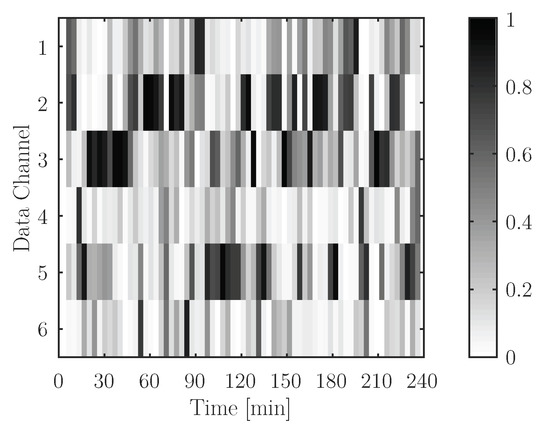
Figure 4.
Time dependence of the channel contribution for 2016/072/00-04.
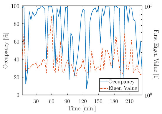
Figure 5.
Occupancy rate and eigenvalue for 2016/72/00-04.
Here, we denoted the time from Y to Z of the Xth day in 2016 as “2016/X/Y-Z.” In Figure 4, the horizontal axis is the time whose origin is 2016/072/00 and the vertical axis is composed of the channel number i. (Unfortunately, the data from 22:30 in the 72nd day to 10:30 the 91st day are not available due to a malfunction of the observatory.) As seen, the random contribution is confirmed for the time far from the Mie earthquake.
At the beginning, we show the time dependence of the channel contribution around the Mie earthquake as contour plot in Figure 6.
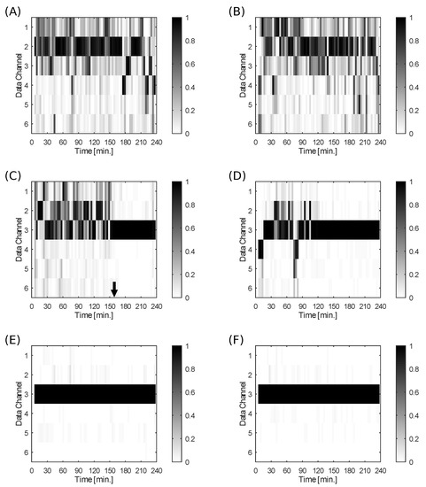
Figure 6.
Transition of the eigenstate around the Mie earthquake for (A) 2016/091/16-19, (B) 2016/091/20-24, (C) 2016/092/00-04, (D) 2016/92/04-08, (E) 2016/92/08-12, (F) 2016/92/12-16. The down arrow shows the time the earthquake occurred.
While the state 20 days before the earthquake shown in Figure 4 has a random contribution, the state of some hours before the earthquake is shown in Figure 6A,B, and it has a strong contribution from channels 1 to 3. Then, the state of several tens of minutes before the earthquake is shown in Figure 6C and it has a strong contribution from channels 2 and 3. Thus, it seems that the contribution from channels 1, 2, and 3 increase before the earthquake. After the earthquake, the eigenstate is mainly consists of channel 3, which is considered due to a change of a crustal state. The first eigenvalue, i.e., the first eigenvalue, has a sharp peak at the time the earthquake occurred in Figure 7C. As shown in Figure 7C, the occupancy rate remains high several tens of minutes before the earthquake.
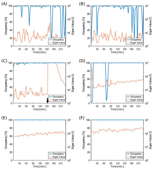
Figure 7.
Occupancy rate and the first eigenvalue around the Mie earthquake for (A) 2016/091/16-19, (B) 2016/091/20-24, (C) 2016/092/00-04, (D) 2016/92/04-08, (E) 2016/92/08-12, (F) 2016/92/12-16. The down arrow shows the time the earthquake occurred.
Next, we show the case of the Kumamoto earthquake. Except around earthquake, the contribution from channel 1 and 2 is always high, as shown in Figure 8. However, the time in which the occupancy rate keeps almost 100% is longer before the earthquake (Figure 9A,B) than after the earthquake (Figure 9E,F).
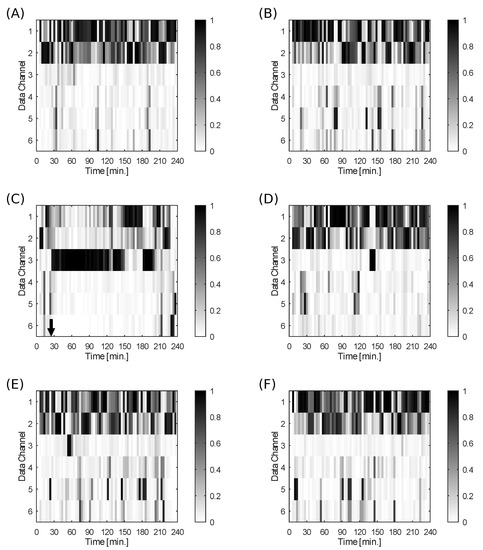
Figure 8.
Transition of the eigenstate around the Kumamoto earthquake for (A) 2016/106/8-12, (B) 2016/106/12-16, (C) 2016/106/16-20, (D) 2016/106/20-24, (E) 2016/107/0-4, (F) 2016/107/4-8.
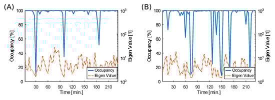
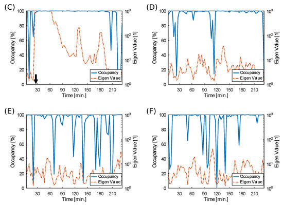
Figure 9.
Occupancy rate and the first eigenvalue around the Kumamoto earthquake for (A) 2016/106/8-12, (B) 2016/106/12-16, (C) 2016/106/16-20, (D) 2016/106/20-24, (E) 2016/107/0-4, (F) 2016/107/4-8.
Finally, we show the results of the Fukushima earthquakes in Figure 10 and Figure 11. At the beginning of the analyzed time, channel 3 has already mainly contributed to the eigenstate while channel 1 and 2 slightly contribute. After that, the states keeps until the end of analyzed time. On the other hand, as seen in Figure 11, eigenvalue shows a similar behavior with EWSs. Namely the first eigenvalue increases from 8 h before the earthquake, and is calm down after the earthquake.
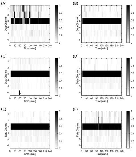
Figure 10.
Transition of the eigenstate around the Fukushima earthquake for (A) 2016/326/12-16, (B) 2016/326/16-20, (C) 2016/326/20-24, (D) 2016/327/00-04, (E) 2016/327/04-08, (F) 2016/327/08-12.
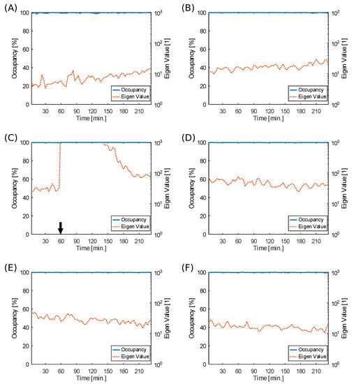
Figure 11.
Occupancy rate and the first eigenvalue around the Fukushima earthquake for (A) 2016/326/12-16, (B) 2016/326/16-20, (C) 2016/326/20-24, (D) 2016/327/00-04, (E) 2016/327/04-08, (F) 2016/327/08-12.
4. Discussion
We discuss the relation between the analytical results and earthquake locations. In the case of the Mie earthquake, we obtain an eigenstate transition of the covariance matrix such as a concentration of the contribution from specific channels immediately around the earthquakes. This shows that an increase in the occupancy rate corresponds to a preceding signal of the an earthquake. It seems that the proximity of this earthquake to the observatory KMDB1 results in this state change. In the case of the Kumamoto earthquake, we could not capture the explicit dominant state as shown in Figure 9A,B. However, the time in which the occupancy rate stays almost 100% is longer before the earthquake (Figure 9A,B) than after the earthquake (Figure 9E,F). This is possibly attributed to the distance between the earthquake and observatory. The observed waveform of DONET is the sum of the activity of various locations with weights depending on the distance. Thus, it is natural to assume that the weights are smaller when the distance is longer. Hence, even if earthquake activity of a far-away point becomes active, its effect on the eigenstate is not direct but reduced by the near-point activity. Thus, the eigenstate shown in Figure 8A,B is interpreted as the combination of a random contribution from the usual earthquake activity from the near point and the dominant state of specific channels before the Kumamoto earthquake. On the other hand, in the case of the Fukushima earthquake which is as far as Kumamoto case, we could not find such randomness. Namely, the concentration from specific channels in eigenstate already starts to occur at the beginning of the analyzed time as shown in Figure 10. Moreover, the eigenvalue increased before the earthquake (Figure 11). Even though we do not have a criteria value to judge earthquake occurrence about the eigenvalue, these behaviors could be interpreted as preceding signals. However, the reason why there is a difference between Kumamoto and Fukushima even though they are both far away from DONET station is an open question.
We analyzed three different earthquakes in which DONET was able to observe the earthquake waveform obtained a common transition of the eigenstate, i.e., the concentration of contribution from the specific channel in the eigenstates. This transition possibly becomes a preceding signal because the concentration to some channels precedes earthquakes at a few hours’ scale. However, using only qualitative analysis of this transition is not sufficient for being useful in preceding signals in practice.
For future work, quantitative analysis of this transition is required such as the relation between the time concentration maintenance and the closeness or magnitude of earthquakes by analyzing many more earthquakes. Furthermore, it is expected that we are able to extract more information by comparing transitions of eigenstates developed from data of different observatories. Noting the relation between the results of our study and EWS methods, as described in the introduction, the EWS method results in an increase in the first eigenvalue and the weights of variables related to a transition. In our study, even though an increasing eigenvalue is confirmed only in the Fukushima earthquake, the concentration in specific channels, which precedes earthquakes, is shown. The data of typical earthquake activity fluctuate and include observational noise because of a requirement to maintain high sensitivity. Thus, it is more difficult to differentiate fluctuation before a transition and observational noise than that of other fields. Thus, it is possible that a difference between our results and the EWS method occurs. For such a system, EWS methods based on a state space model, in which an observational model and physical model are treated, may be required.
There are other studies that focus on the aspect that earthquakes are critical phenomena. For example, regarding earthquake occurrence as point process, small earthquakes before large earthquakes were analyzed by the means of multiresolution wavelet analysis and natural time analysis [22]. It is proposed that we could know whether the crustal state is at a critical stage of earthquake occurrence by extracting critical parameters. Although the timescales they are focusing on are different from us, there is a possibility that they can be discussed on the basis of a common root, such as a micro model of earthquake, in the future. Another study considered multiple strain gauges installed at distant locations, that is wide area information, as a network, and captured the topological changes in the network structure before an earthquake occurs [23]. Their study considered multiple strain gauges at different locations as multi-channel and uses multi-channel anomaly spectrum analysis. On the other hand, we tried to capture the precursors of earthquakes from local multi-physical quantity relationships. It would be useful for developing our study to capture seismic activity with wide area information. There is a possibility that it enables estimating more information such as the location and timing of earthquake occurrence. Then, in order to discuss the relationship between time series data at spatially distant locations, spatial data interpolation techniques [24] would be necessary.
5. Conclusions
In this study, we analyzed the eigenstate of the covariance matrix developed from multi-channel time series data of DONET. We validated the possibility of using the eigenstate as a preceding signal comparing past earthquakes and the transition of the eigenstate on the basis of the EWS concept. As a result, it was confirmed that the concentration of the contribution to the eigenstate from specific channels or the first eigenvalue precedes earthquakes. Though this change possibly becomes a preceding signal, this qualitative analysis is not sufficient for practical usage because of the lack of specific criteria for earthquake occurrence. Thus, a quantitative analysis of this transition is required, such as the relation between the concentration maintenance time and the closeness or magnitude of earthquakes by analyzing many more earthquakes. Furthermore, it is expected to extract more information by comparing transitions of eigenstates developed by data obtained from different location observatories. These works will be promoted when the observation network develops in the future.
Author Contributions
Conceptualization, A.O. and Y.K.; Investigation, A.O.; Supervision, Y.K.; Writing—original draft, A.O.; Writing—review & editing, Y.K. All authors have read and agreed to the published version of the manuscript.
Funding
This research was not supported by any granting agency or foundation, nor by any third-party donations.
Institutional Review Board Statement
Not applicable.
Informed Consent Statement
Not applicable.
Data Availability Statement
The data we used in this study are available by requesting JAMSTEC on their website (J-SEIS, https://join-web.jamstec.go.jp/join-portal/, accessed on 25 July 2019).
Acknowledgments
We would like to thank JAMSTEC for their data publicly available.
Conflicts of Interest
Author A.O. was employed by the company Toyota Central Research and Development Laboratories, Inc. The remaining author declares that the research was conducted in the absence of any commercial or financial relationships that could be construed as a potential conflict of interest.
Abbreviations
| The following abbreviations are used in this manuscript: | |
| EWS | Early warning signals |
| DONET | Dense Oceanfloor network |
| JAMSTEC | Japan agency for marine-earth science and technology |
| SEED | Standard for the exchange of earthquake data |
References
- Enomoto, Y.; Yamabe, T.; Okumura, N. Causal mechanisms of seismo-EM phenomena during the 1965–1967 Matsushiro earthquake swarm. Sci. Rep. 2017, 7, 44774. [Google Scholar] [CrossRef] [PubMed] [Green Version]
- Orihara, Y.; Kamogawa, M.; Nagao, T. Preseismic Changes of the Level and Temperature of Confined Groundwater related to the 2011 Tohoku Earthquake. Sci. Rep. 2014, 4, 6907. [Google Scholar] [CrossRef] [PubMed] [Green Version]
- Varotsos, P.; Alexopoulos, K. Physical properties of the variations of the electric field of the earth preceding earthquakes. II. determination of epicenter and magnitude. Tectonophysics 1984, 110, 99–125. [Google Scholar] [CrossRef]
- Uyeda, S.; Nagao, T.; Kamogawa, M. Short-term earthquake prediction: Current status of seismo-electromagnetics. Tectonophysics 2009, 470, 205–213. [Google Scholar] [CrossRef]
- Molchanov, O.A.; Hayakawa, M.; Oudoh, T.; Kawai, E. Precursory effects in the subionospheric VLF signals for the Kobe earthquake. Phys. Earth Planet. Inter. 1998, 105, 239–248. [Google Scholar] [CrossRef]
- Murai, S. Can we predict earthquakes with GPS data? Int. J. Digit. Earth 2010, 3, 83–90. [Google Scholar] [CrossRef]
- He, L.; Heki, K. Three-Dimensional Tomography of Ionospheric Anomalies Immediately Before the 2015 Illapel Earthquake, Central Chile. J. Geophys. Res. Space Phys. 2018, 123, 4015–4025. [Google Scholar] [CrossRef] [Green Version]
- He, L.; Heki, K.; Wu, L. Three-Dimensional and Trans-Hemispheric Changes in Ionospheric Electron Density Caused by the Great Solar Eclipse in North America on 21 August 2017. Geophys. Res. Lett. 2018, 45, 10933–10940. [Google Scholar] [CrossRef] [Green Version]
- Ide, S.; Yabe, S.; Tanaka, Y. Earthquake potential revealed by tidal influence on earthquake size-frequency statistics. Nat. Geosci. 2016, 9, 834–837. [Google Scholar] [CrossRef]
- Mignan, A.; Broccardo, M. Neural Network Applications in Earthquake Prediction (1994–2019): Meta-Analytic and Statistical Insights on Their Limitations. Seismol. Res. Lett. 2020, 91, 2330–2342. [Google Scholar] [CrossRef]
- Moustra, M.; Avraamides, M.; Christodoulou, C. Artificial neural networks for earthquake prediction using time series magnitude data or Seismic Electric Signals. Expert Syst. Appl. 2011, 38, 15032–15039. [Google Scholar] [CrossRef]
- Külahcı, F.; İnceöz, M.; Doğru, M.; Aksoy, E.; Baykara, O. Artificial neural network model for earthquake prediction with radon monitoring. Appl. Radiat. Isot. 2009, 67, 212–219. [Google Scholar] [CrossRef] [PubMed]
- Scheffer, M.; Bascompte, J.; Brock, W.A.; Brovkin, V.; Carpenter, S.R.; Dakos, V.; Held, H.; van Nes, E.H.; Rietkerk, M.; Sugihara, G. Early-warning signals for critical transitions. Nature 2009, 461, 53–59. [Google Scholar] [CrossRef] [PubMed]
- Chen, L.; Liu, R.; Liu, Z.P.; Li, M.; Aihara, K. Detecting early-warning signals for sudden deterioration of complex diseases by dynamical network biomarkers. Sci. Rep. 2012, 2, 342. [Google Scholar] [CrossRef] [PubMed] [Green Version]
- Oku, M.; Aihara, K. On the covariance matrix of the stationary distribution of a noisy dynamical system. Nonlinear Theory Its Appl. IEICE 2018, 9, 166–184. [Google Scholar] [CrossRef] [Green Version]
- Matsumori, T.; Sakai, H.; Aihara, K. Early-warning signals using dynamical network markers selected by covariance. PRE 2019, 100, 052303. [Google Scholar] [CrossRef] [PubMed]
- Kaneda, Y.; Kawaguchi, K.; Araki, E.; Matsumoto, H.; Nakamura, T.; Kamiya, S.; Ariyoshi, K.; Hori, T.; Baba, T.; Takahashi, N.; et al. Development and application of an advanced ocean floor network system for megathrust earthquakes and tsunamis. In Seafloor Observatories: A New Vision of the Earth from the Abyss; Springer: Berlin/Heidelberg, Germany, 2015; pp. 643–662. [Google Scholar] [CrossRef]
- Kawaguchi, K.; Kaneko, S.; Nishida, T.; Komine, T.; Favali, P.; Beranzoli, L.; De Santis, A. Construction of the DONET real-time seafloor observatory for earthquakes and tsunami monitoring. In Seafloor Observatories: A New Vision of the Earth from the Abyss; Springer: Berlin/Heidelberg, Germany, 2015; pp. 211–228. [Google Scholar] [CrossRef]
- Incorporated Research Institutions for Seismology. Manuals: Rdseed. Available online: https://ds.iris.edu/ds/nodes/dmc/manuals/rdseed/ (accessed on 25 July 2019).
- Japan Meteorological Agency. CMT Solution. Available online: https://www.data.jma.go.jp/svd/eqev/data/mech/cmt/cmt201604.html (accessed on 24 November 2021).
- Eaton, J.W.; Bateman, D.; Hauberg, S.; Wehbring, R. GNU Octave Version 5.1.0 Manual: A High-Level Interactive Language for Numerical Computations. Available online: https://www.gnu.org/software/octave/doc/v5.1.0/ (accessed on 25 July 2019).
- Vallianatos, F.; Michas, G.; Hloupis, G. Seismicity Patterns Prior to the Thessaly (Mw6.3) Strong Earthquake on 3 March 2021 in Terms of Multiresolution Wavelets and Natural Time Analysis. Geosciences 2021, 11, 379. [Google Scholar] [CrossRef]
- Yu, Z.; Hattori, K.; Zhu, K.; Chi, C.; Fan, M.; He, X. Detecting Earthquake-Related Anomalies of a Borehole Strain Network Based on Multi-Channel Singular Spectrum Analysis. Entropy 2020, 22, 1086. [Google Scholar] [CrossRef] [PubMed]
- Ghaderpour, E. Multichannel antileakage least-squares spectral analysis for seismic data regularization beyond aliasing. Acta Geophys. 2019, 67, 1349–1363. [Google Scholar] [CrossRef]
Publisher’s Note: MDPI stays neutral with regard to jurisdictional claims in published maps and institutional affiliations. |
© 2021 by the authors. Licensee MDPI, Basel, Switzerland. This article is an open access article distributed under the terms and conditions of the Creative Commons Attribution (CC BY) license (https://creativecommons.org/licenses/by/4.0/).