
Fundus Image Registration Technique Based on Local Feature of Retinal Vessels

 , and
, and
Abstract
:1. Introduction
2. Related Works
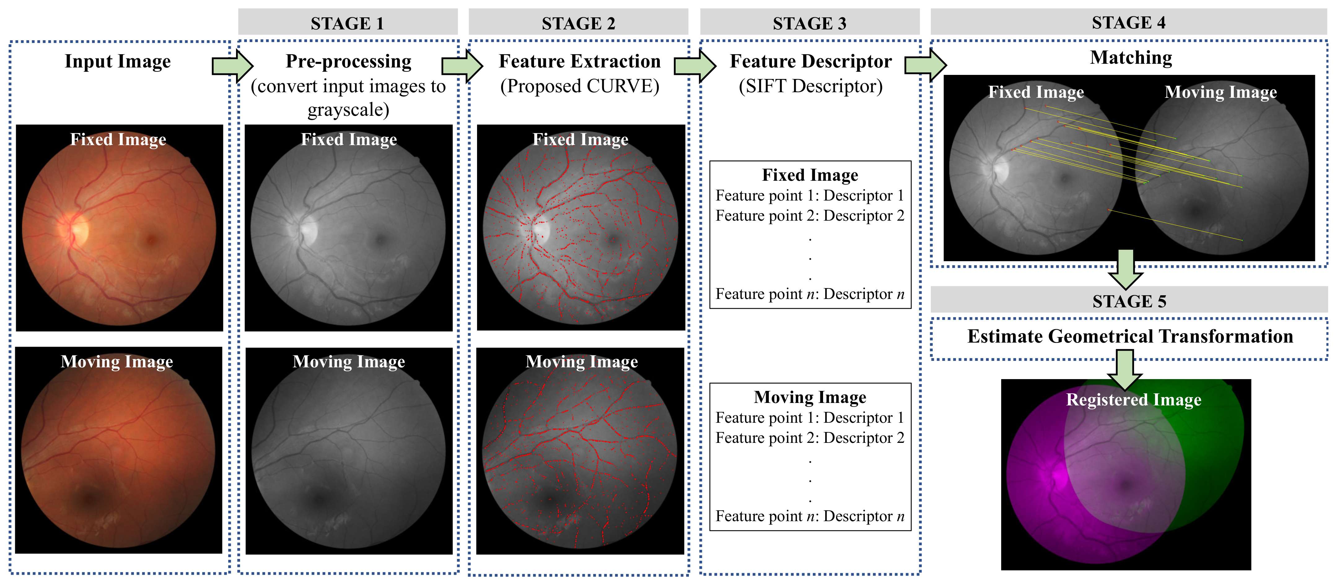
3. Methodology
3.1. STAGE 1: Pre-Processing
3.2. STAGE 2: Feature Extraction
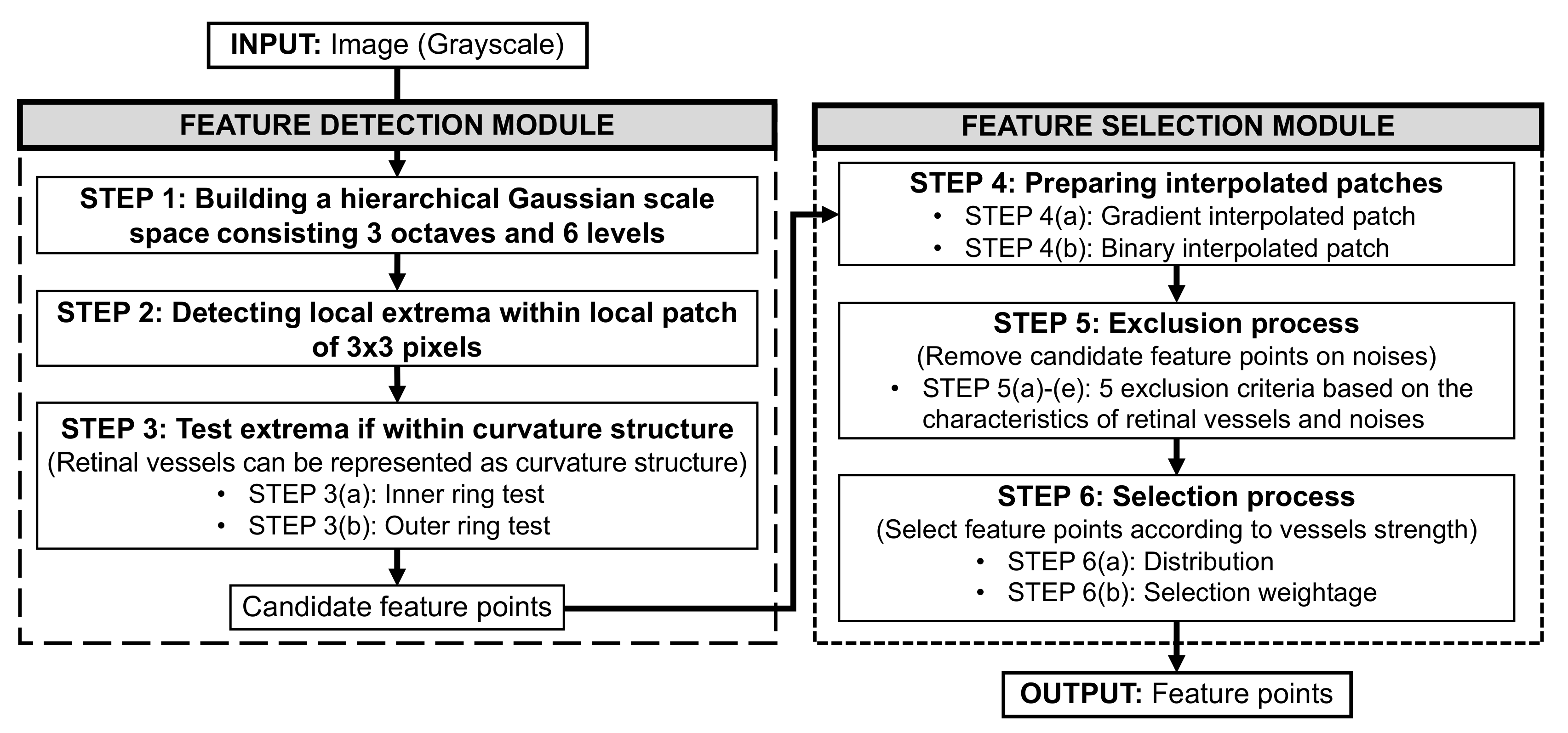
3.2.1. Feature Detection Module
- (a)
- STEP 1: Building a hierarchical Gaussian scale space
- (b)
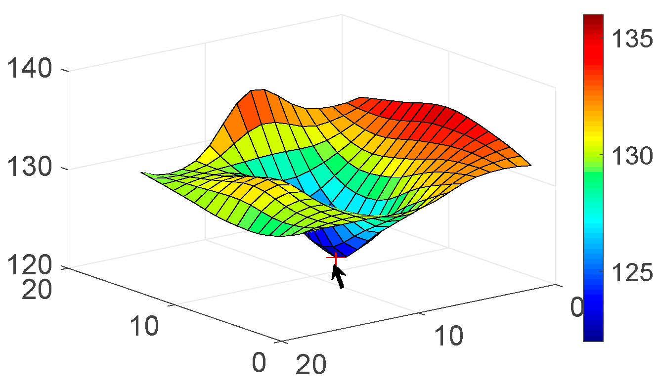
- STEP 2: Detecting local extrema
- (c)
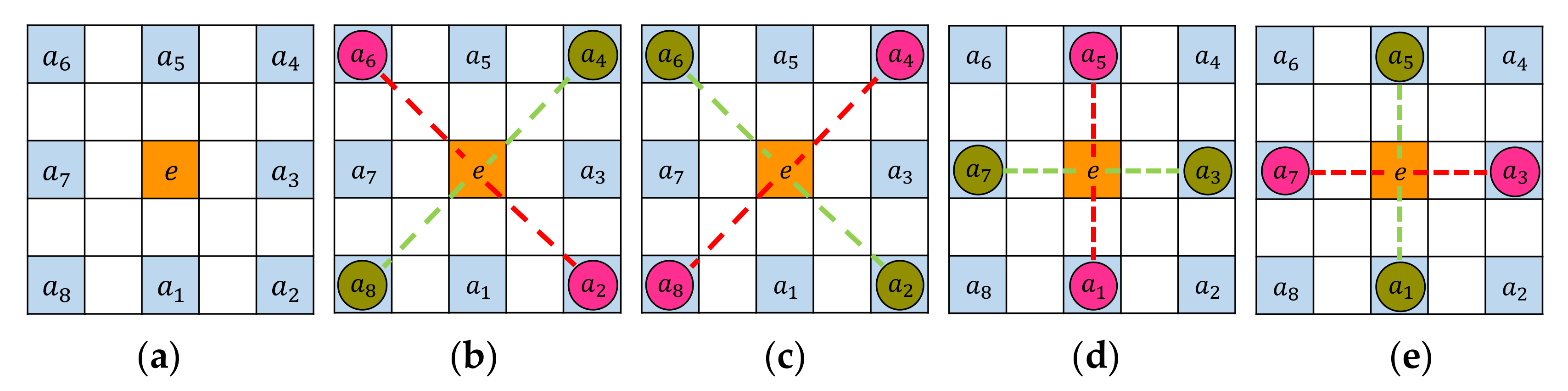
- STEP 3: Test extrema if within curvature structure
- STEP 3(a): Inner ring test
- STEP 3(b): Outer ring test
3.2.2. Feature Selection Module
- (a)
- STEP 4: Preparing gradient and binary interpolated patches
- (b)
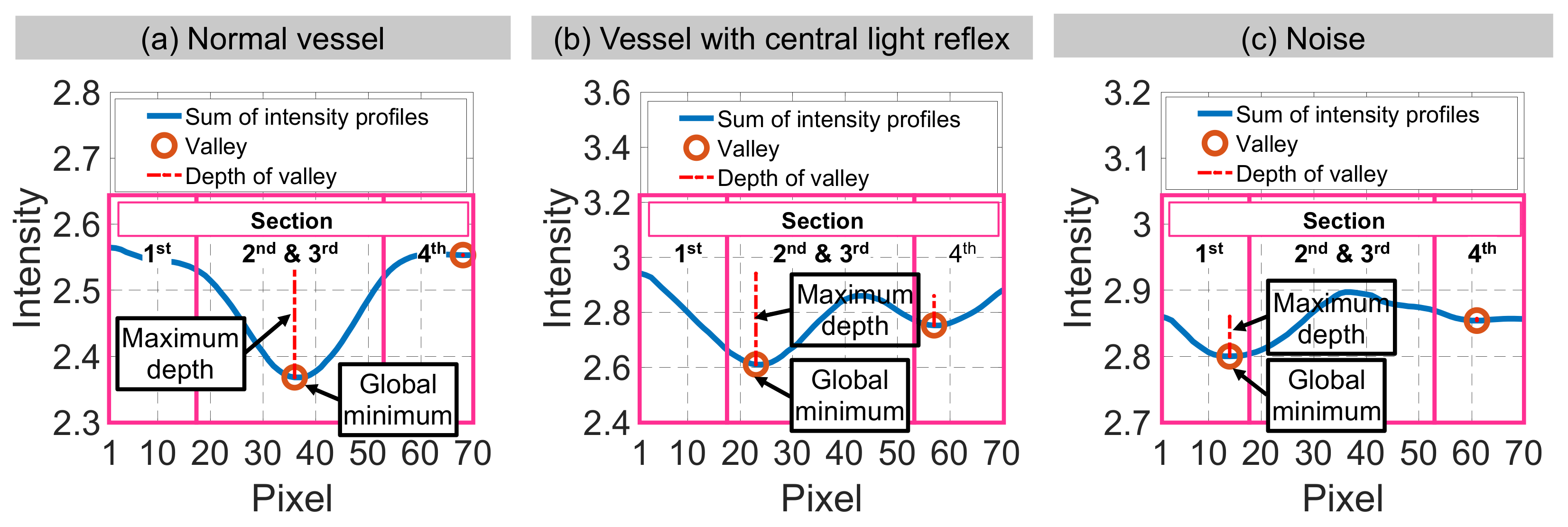
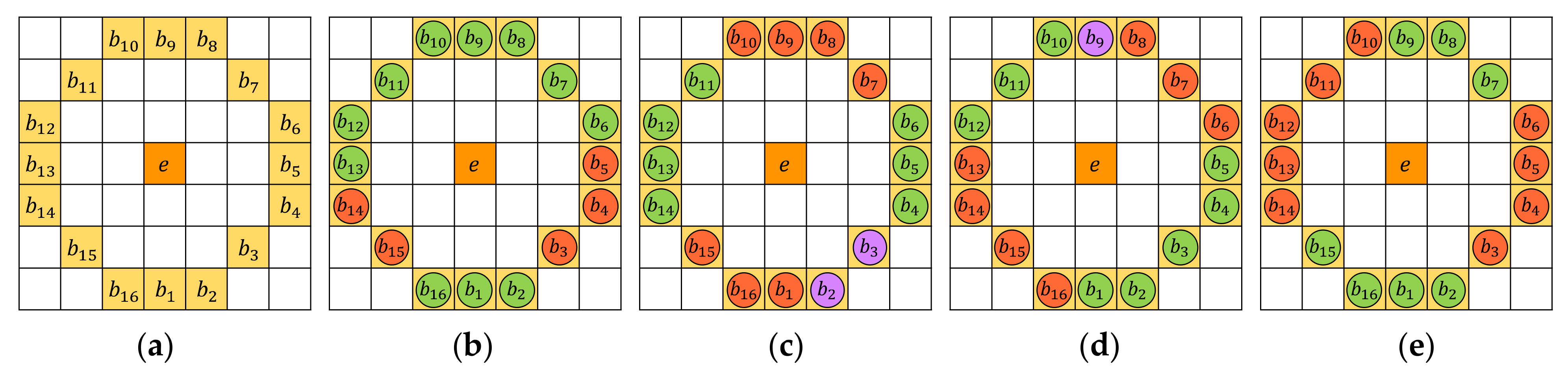
- STEP 5: Exclusion process
- STEP 5(a): Exclusion criterion 1
- STEP 5(b): Exclusion criterion 2
- STEP 5(c): Exclusion criterion 3
- STEP 5(d): Exclusion criterion 4
- STEP 5(e): Exclusion criterion 5
- (c)
- STEP 6: Selection process
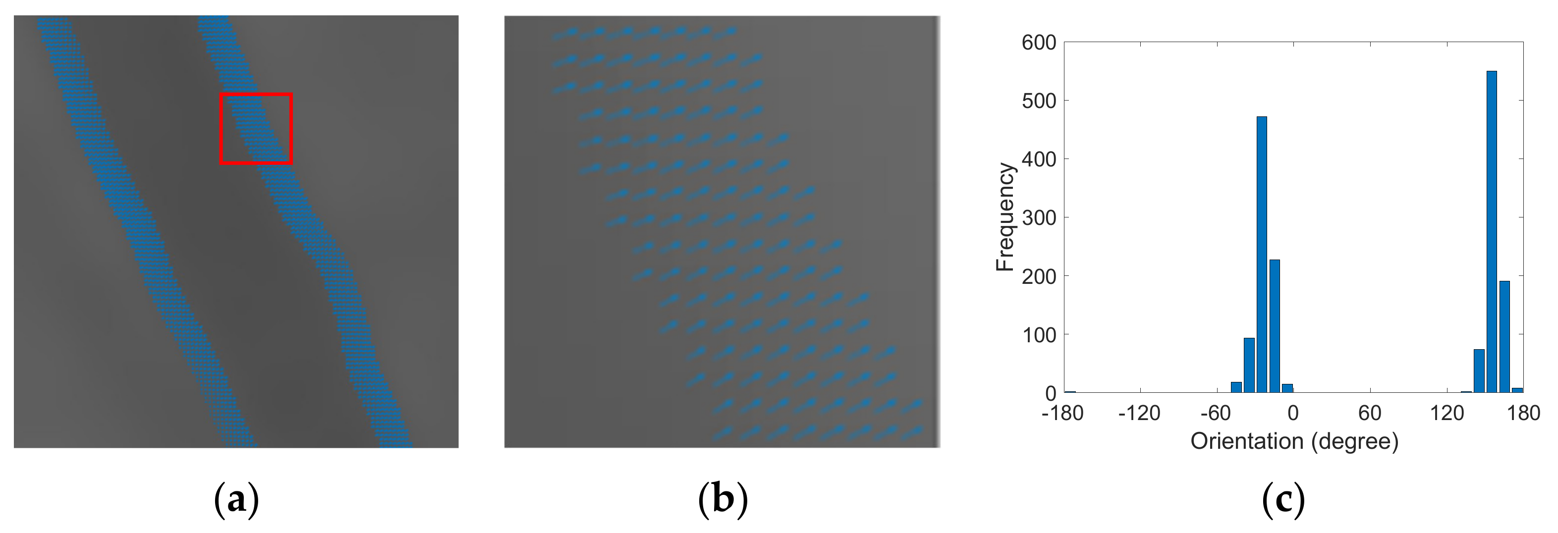
- STEP 6(a): Distribution
- STEP 6(b): Selection weightage
3.3. STAGE 3: Feature Descriptor
3.4. STAGE 4: Matching
3.5. STAGE 5: Geometrical Transformation
4. Experimental Setup
4.1. Datasets
4.2. Evaluation Metrics
4.2.1. Feature Extraction Performance
- (a)
- Extraction accuracy
- (b)
- Factors influencing the extraction accuracy
4.2.2. Registration Performance
- (a)
- Success rate
- (b)
- Factors influencing the success rate
5. Results
5.1. Feature Extraction Performance
5.2. Registration Performance
6. Conclusions
Author Contributions
Funding
Institutional Review Board Statement
Informed Consent Statement
Data Availability Statement
Conflicts of Interest
Appendix A

| No. | Symbol | Description | No. | Symbol | Description |
|---|---|---|---|---|---|
| 1 | . | 28 | Distance between the parallel cross-sectional lines. pixels. | ||
| 2 | Central intensity value. | 29 | Length of the cross-sectional lines. | ||
| 3 | . | 30 | Total of the cross-sectional lines, an odd number. pixels. | ||
| 4 | Constant factor. | 31 | Index of the feature point. | ||
| 5 | . | 32 | Index of the images in the hierarchical Gaussian scale space. | ||
| 6 | . | 33 | |||
| 7 | . | 34 | |||
| 8 | for inner ring test. | 35 | |||
| 9 | Area of the intersected region between the sums of intensity profiles from the gradient and binary interpolated patches. | 36 | |||
| 10 | for outer ring test. | 37 | |||
| 11 | The blue channel. | 38 | |||
| 12 | . | 39 | |||
| 13 | Extremum. | 40 | The red channel. | ||
| 14 | Entropy of a grid image. | 41 | Side length of the binary interpolated patch. | ||
| 15 | Entropy of a gradient interpolated patch. | 42 | . | ||
| 16 | . | 43 | |||
| 17 | . | 44 | |||
| 18 | The green channel. | 45 | Total candidate feature points detected in a grid image. | ||
| 19 | Hierarchical Gaussian scale space. | 46 | |||
| 20 | . | 47 | |||
| 21 | Index of the candidate feature point in a Gaussian image. | 48 | Peak deviation nonuniformity of a grid image. | ||
| 22 | Input image in grayscale. | 49 | |||
| 23 | . | 50 | |||
| 24 | . | 51 | |||
| 25 | . | 52 | |||
| 26 | . | 53 | |||
| 27 | . | 54 |
Appendix B
| (i) Colour Patch | (ii) Grayscale Patch | (iii) Intensity Profile for (ii) | (iv) Binary Patch | (v) Intensity Profile for (iv) | (vi) Grayscale Patch in 3-D | |
|---|---|---|---|---|---|---|
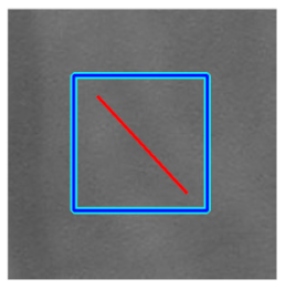
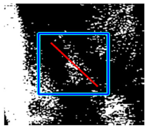
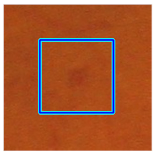
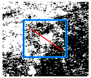
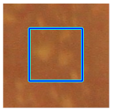
| Retinal Vessels |  (a) Retinal vessel without central light reflex |  |  |  |  | 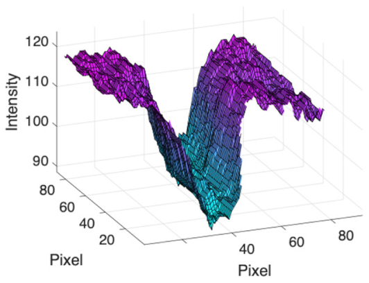 |
 |  |  |  | |||
 (b) Retinal vessel with central light reflex | 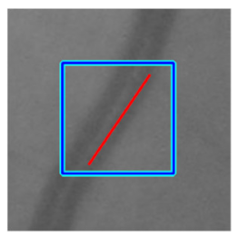 | 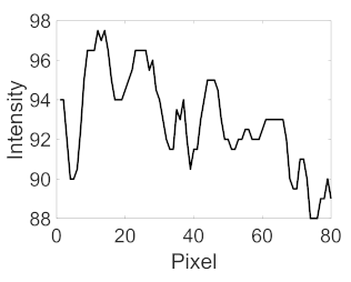 | 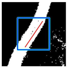 | 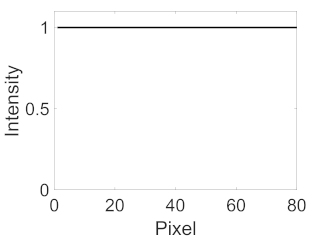 | 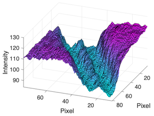 | |
 |  |  |  | |||
| Noise | (i) Colour Patch | (ii) Grayscale Patch | (iii) Intensity Profile for (ii) | (iv) Binary Patch | (v) Intensity Profile for (iv) | (vi) Grayscale Patch in 3-D |
 (c) Retinal nerve fibre layer | 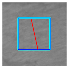 | 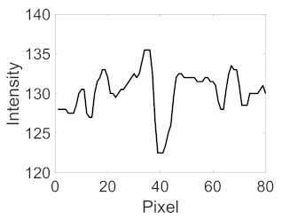 | 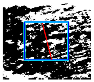 | 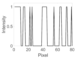 | 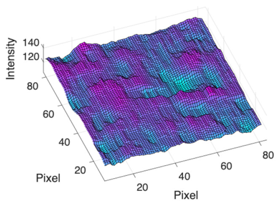 | |
 |  |  |  | |||
 (d) Single underlying choroidal vessels | 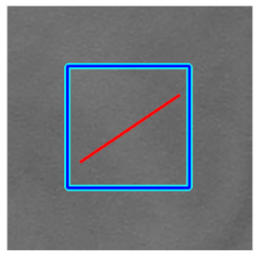 | 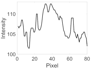 | 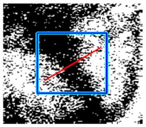 |  | 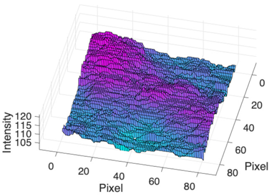 | |
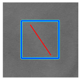 |  |  |  | |||
| Noise | (i) Colour Patch | (ii) Grayscale Patch | (iii) Intensity Profile for (ii) | (iv) Binary Patch | (v) Intensity Profile for (iv) | (vi) Grayscale Patch in 3-D |
 (e) Multiple underlying choroidal vessels |  | 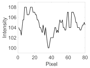 | 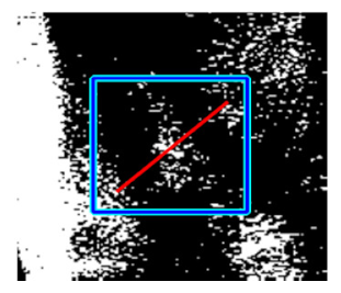 |  | 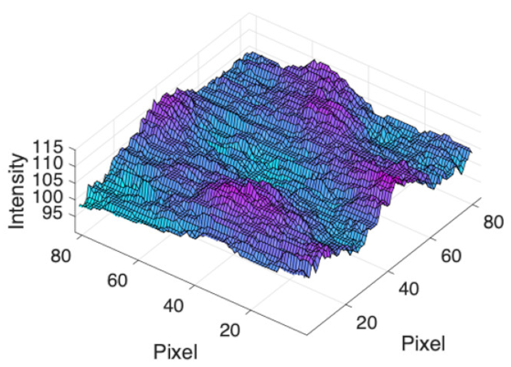 | |
 |  |  |  | |||
 (f) Microaneurysm | 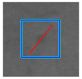 |  | 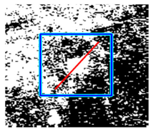 | 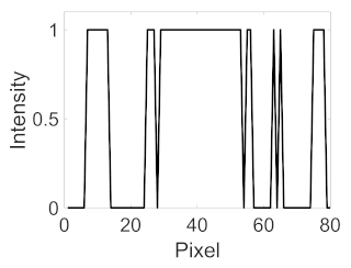 | 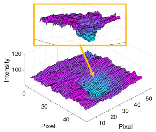 | |
 |  |  |  | |||
| Noise | (i) Colour Patch | (ii) Grayscale Patch | (iii) Intensity Profile for (ii) | (iv) Binary Patch | (v) Intensity Profile for (iv) | (vi) Grayscale Patch in 3-D |
 (g) Exudates |  | 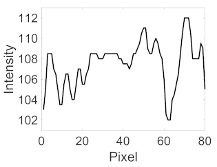 | 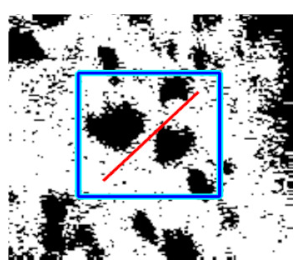 | 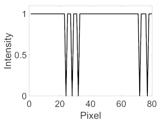 | 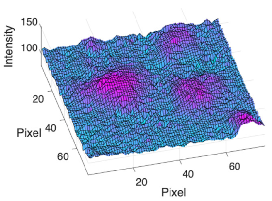 | |
 |  |  |  | |||
 (h) Edge of optic disc |  | 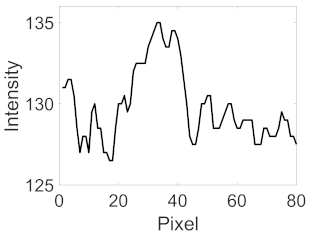 | 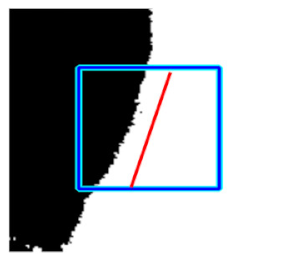 |  | 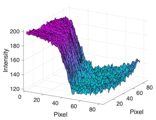 | |
 |  |  |  |
References
- Hernandez-Matas, C.; Zabulis, X.; Argyros, A.A. Retinal image registration as a tool for supporting clinical applications. Comp. Meth. Prog. Biomed. 2021, 199, 105900. [Google Scholar] [CrossRef] [PubMed]
- Legg, P.A.; Rosin, P.L.; Marshall, D.; Morgan, J.E. Improving accuracy and efficiency of mutual information for multi-modal retinal image registration using adaptive probability density estimation. Comput. Med. Imaging. Graph. 2013, 37, 597–606. [Google Scholar] [CrossRef] [PubMed] [Green Version]
- Nakagawa, T.; Suzuki, T.; Hayashi, Y.; Mizukusa, Y.; Hatanaka, Y.; Ishida, K.; Hara, T.; Fujita, H.; Yamamoto, T. Quantitative depth analysis of optic nerve head using stereo retinal fundus image pair. J. Biomed. Opt. 2008, 13, 064026. [Google Scholar] [CrossRef] [PubMed] [Green Version]
- Kolar, R.; Sikula, V.; Base, M. Retinal Image Registration using Phase Correlation. Anal. Biomed. Signals Images 2010, 20, 244–252. [Google Scholar] [CrossRef]
- Kolar, R.; Harabis, V.; Odstrcilik, J. Hybrid retinal image registration using phase correlation. Imaging Sci. J. 2013, 61, 369–384. [Google Scholar] [CrossRef]
- Chanwimaluang, T.; Fan, G.L.; Fransen, S.R. Hybrid Retinal Image Registration. IEEE Trans. Inf. Technol. Biomed. 2006, 10, 129–142. [Google Scholar] [CrossRef]
- Zitova, B.; Flusser, J. Image registration methods: A survey. Image Vis. Comput. 2003, 21, 977–1000. [Google Scholar] [CrossRef] [Green Version]
- Ghassabi, Z.; Shanbehzadeh, J.; Mohammadzadeh, A.; Ostadzadeh, S.S. Colour retinal fundus image registration by selecting stable extremum points in the scale–Invariant feature transform detector. IET Image Process. 2015, 9, 889–900. [Google Scholar] [CrossRef]
- Hernandez-Matas, C.; Zabulis, X.; Argyros, A.A. An Experimental Evaluation of the Accuracy of Keypoints-Based Retinal Image Registration. In Proceedings of the 39th Annual International Conference of the IEEE Engineering in Medicine and Biology Society (EMBC), Seogwipo, Korea, 11–15 July 2017; pp. 377–381. [Google Scholar]
- Chen, J.; Chen, J.; Tian, J.; Lee, N.; Zheng, J.; Smith, R.T.; Laine, A.F. A Partial Intensity Invariant Feature Descriptor for Multimodal Retinal Image Registration. IEEE Trans. Biomed. Eng. 2010, 57, 1707–1718. [Google Scholar] [CrossRef] [Green Version]
- Ghassabi, Z.; Shanbehzadeh, J.; Sedaghat, A.; Fatemizadeh, E. An efficient approach for robust multimodal retinal image registration based on UR-SIFT features and PIIFD descriptors. Eurasip. J. Image Video Process. 2013, 2013, 25. [Google Scholar] [CrossRef] [Green Version]
- Ramli, R.; Idris, M.Y.I.; Hasikin, K.; Karim, N.K.A. Histogram-Based Threshold Selection of Retinal Feature for Image Registration. In Proceedings of the 3rd International Conference on Information Technology & Society (IC-ITS), Penang, Malaysia, 31 July–1 August 2017; pp. 105–114. [Google Scholar]
- Yang, G.; Stewart, C.V.; Sofka, M.; Tsai, C.-L. Registration of challenging image pairs: Initialization, estimation, and decision. IEEE Trans. Pattern Anal. Mach. Intell. 2007, 29, 1973–1989. [Google Scholar] [CrossRef] [PubMed] [Green Version]
- Ramli, R.; Idris, M.Y.I.; Hasikin, K.; Karim, N.K.A.; Abdul Wahab, A.W.; Ahmedy, I.; Ahmedy, F.; Kadri, N.A.; Arof, H. Feature-Based Retinal Image Registration Using D-Saddle Feature. J. Healthc. Eng. 2017, 2017, 1489524. [Google Scholar] [CrossRef] [PubMed] [Green Version]
- Lowe, D.G. Distinctive image features from scale-Invariant keypoints. Int. J. Comput. Vis. 2004, 60, 91–110. [Google Scholar] [CrossRef]
- Hernandez-Matas, C.; Zabulis, X.; Argyros, A.A. Retinal image registration through simultaneous camera pose and eye shape estimation. In Proceedings of the 38th Annual International Conference of the IEEE Engineering in Medicine and Biology Society (EMBC), Orlando, FL, USA, 16–20 August 2016; pp. 3247–3251. [Google Scholar]
- Hernandez-Matas, C.; Zabulis, X.; Triantafyllou, A.; Anyfanti, P.; Argyros, A.A. Retinal image registration under the assumption of a spherical eye. Comput. Med. Imaging Graph. 2017, 55, 95–105. [Google Scholar] [CrossRef] [PubMed]
- Tsai, C.; Li, C.; Yang, G.; Lin, K. The Edge-Driven Dual-Bootstrap Iterative Closest Point Algorithm for Registration of Multimodal Fluorescein Angiogram Sequence. IEEE Trans. Med. Imaging. 2010, 29, 636–649. [Google Scholar]
- Sedaghat, A.; Mokhtarzade, M.; Ebadi, H. Uniform robust scale-Invariant feature matching for optical remote sensing images. IEEE Trans. Geosci. Remote. Sens. 2011, 49, 4516–4527. [Google Scholar] [CrossRef]
- Frangi, A.F.; Niessen, W.J.; Vincken, K.L.; Viergever, M.A. Multiscale vessel enhancement filtering. In Proceedings of the International Conference on Medical Image Computing and Computer-Assisted Intervention (MICCAI’98), Cambridge, MA, USA, 11–13 October 1998. [Google Scholar]
- Vonikakis, V.; Chrysostomou, D.; Kouskouridas, R.; Gasteratos, A. A biologically inspired scale-Space for illumination invariant feature detection. Meas. Sci. Technol. 2013, 24, 074024. [Google Scholar] [CrossRef] [Green Version]
- Lee, J.A.; Cheng, J.; Hai Lee, B.; Ping Ong, E.; Xu, G.; Wing Kee Wong, D.; Liu, J.; Laude, A.; Han Lim, T. A low-Dimensional step pattern analysis algorithm with application to multimodal retinal image registration. In Proceedings of the IEEE Conference on Computer Vision and Pattern Recognition (CVPR), Boston, MA, USA, 7–12 June 2015; pp. 1046–1053. [Google Scholar]
- Wang, G.; Wang, Z.C.; Chen, Y.F.; Zhao, W.D. Robust point matching method for multimodal retinal image registration. Biomed. Signal Process. Control. 2015, 19, 68–76. [Google Scholar] [CrossRef]
- Hernandez-Matas, C.; Zabulis, X.; Argyros, A.A. Retinal image registration based on keypoint correspondences, spherical eye modeling and camera pose estimation. In Proceedings of the 37th Annual International Conference of the IEEE Engineering in Medicine and Biology Society (EMBC), Milan, Italy, 25–29 August 2015; pp. 5650–5654. [Google Scholar]
- Lee, J.A.; Lee, B.H.; Xu, G.; Ong, E.P.; Wong, D.W.K.; Liu, J.; Lim, T.H. Geometric corner extraction in retinal fundus images. In Proceedings of the 2014 36th Annual International Conference of the IEEE Engineering in Medicine and Biology Society, Chicago, IL, USA, 26–30 August 2014; pp. 158–161. [Google Scholar]
- Harris, C.; Stephens, M. A combined corner and edge detector. In Proceedings of the 4th Alvey Vision Conference, Manchester, UK, 31 August–2 September 1988; pp. 147–151. [Google Scholar]
- Bay, H.; Tuytelaars, T.; van Gool, L. SURF: Speeded up Robust Features. In Proceedings of the 9th European Conference on Computer Vision (ECCV), Graz, Austria, 7–13 May 2006; pp. 404–417. [Google Scholar]
- Bay, H.; Ess, A.; Tuytelaars, T.; Van Gool, L. Speeded-Up Robust Features (SURF). Comput. Vis. Image Underst. 2008, 110, 346–359. [Google Scholar] [CrossRef]
- International Telecommunication Union. Studio encoding parameters of digital television for standard 4:3 and wide-Screen 16: 9 aspect ratios. In Recommendation ITU-R BT.601–7; ITU: Geneva, Switzerland, 2017; pp. 1–8. [Google Scholar]
- Kanan, C.; Cottrell, G.W. Color-to-Grayscale: Does the Method Matter in Image Recognition? PLoS ONE 2012, 7, e29740. [Google Scholar] [CrossRef] [Green Version]
- Burger, W.; Burge, M.J. SIFT—Scale-Invariant Local Features. In Principles of Digital Image Processing: Advanced Methods; Springer: London, UK, 2013; pp. 229–295. [Google Scholar]
- Aldana-Iuit, J.; Mishkin, D.; Chum, O.; Matas, J. In the Saddle: Chasing Fast and Repeatable Features. In Proceedings of the 23rd International Conference on Pattern Recognition, Cancun, Mexico, 4–8 December 2016. [Google Scholar]
- CHASE_DB1 Retinal Image Database. Available online: https://blogs.kingston.ac.uk/retinal/chasedb1/ (accessed on 10 December 2017).
- Fraz, M.M.; Remagnino, P.; Hoppe, A.; Uyyanonvara, B.; Rudnicka, A.R.; Owen, C.G.; Barman, S.A. An ensemble classification-Based approach applied to retinal blood vessel segmentation. IEEE Trans. Biomed. Eng. 2012, 59, 2538–2548. [Google Scholar] [CrossRef] [PubMed]
- Staal, J.; Abràmoff, M.D.; Niemeijer, M.; Viergever, M.A.; Van Ginneken, B. Ridge-Based vessel segmentation in color images of the retina. IEEE Trans. Med. Imaging 2004, 23, 501–509. [Google Scholar] [CrossRef]
- DRIVE: Digital Retinal Images for Vessel Extraction. Available online: http://www.isi.uu.nl/Research/Databases/DRIVE/ (accessed on 10 December 2017).
- HRF: High-Resolution Fundus Image Database. Available online: https://www5.cs.fau.de/research/data/fundus-images/ (accessed on 10 December 2017).
- Budai, A.; Bock, R.; Maier, A.; Hornegger, J.; Michelson, G. Robust vessel segmentation in fundus images. Int. J. Biomed. Imaging 2013, 2013, 154860. [Google Scholar] [CrossRef] [Green Version]
- STARE: Structured Analysis of the Retina. Available online: http://cecas.clemson.edu/~ahoover/stare/ (accessed on 10 December 2017).
- Hoover, A.; Kouznetsova, V.; Goldbaum, M. Locating blood vessels in retinal images by piecewise threshold probing of a matched filter response. IEEE Trans. Med. Imaging 2000, 19, 203–210. [Google Scholar] [CrossRef] [PubMed] [Green Version]
- Hernandez-Matas, C.; Zabulis, X.; Triantafyllou, A.; Anyfanti, P.; Douma, S.; Argyros, A.A. FIRE: Fundus Image Registration dataset. J. Modeling Ophthalmol. 2017, 1, 16–28. [Google Scholar] [CrossRef]
- Saha, S.K.; Xiao, D.; Frost, S.; Kanagasingam, Y. A Two-Step Approach for Longitudinal Registration of Retinal Images. J. Med. Syst. 2016, 40, 277. [Google Scholar] [CrossRef]
- Gonzalez, R.C.; Woods, R.E.; Eddins, S.L. Representation and Description. In Digital Image Processing Using MATLAB; Prentice Hall: Hoboken, NJ, USA, 2009. [Google Scholar]
- Goerner, F.L.; Duong, T.; Stafford, R.J.; Clarke, G.D. A comparison of five standard methods for evaluating image intensity uniformity in partially parallel imaging MRI. Med. Phys. 2013, 40, 082302-1–082302-10. [Google Scholar] [CrossRef] [Green Version]
- Brown, M.; Lowe, D.G. Invariant Features from Interest Point Groups. In Proceedings of the British Machine Vision Conference (BMVC), Cardiff, UK, 2–5 September 2002. [Google Scholar]
- Vedaldi, A.; Fulkerson, B. VLFeat: An open and portable library of computer vision algorithms. In Proceedings of the 18th ACM international conference on Multimedia, Firenze, Italy, 25–29 October 2010; pp. 1469–1472. [Google Scholar]
- Torr, P.H.; Zisserman, A. MLESAC: A new robust estimator with application to estimating image geometry. Comput. Vis. Image Underst. 2000, 78, 138–156. [Google Scholar] [CrossRef] [Green Version]
- Goshtasby, A. Image registration by local approximation methods. Image Vis. Comput. 1988, 6, 255–261. [Google Scholar] [CrossRef]
- Pauli, T.W.; Gangaputra, S.; Hubbard, L.D.; Thayer, D.W.; Chandler, C.S.; Peng, Q.; Narkar, A.; Ferrier, N.J.; Danis, R.P. Effect of Image Compression and Resolution on Retinal Vascular Caliber. Investig. Ophthalmol. Vis. Sci. 2012, 53, 5117–5123. [Google Scholar] [CrossRef] [Green Version]
- Brown, D.M.; Ciardella, A. Mosaic Fundus Imaging in the Diagnosis of Retinal Diseases. Investig. Ophthalmol. Vis. Sci. 2005, 46, 2581. [Google Scholar]
- Bontala, A.; Sivaswamy, J.; Pappuru, R.R. Image mosaicing of low quality neonatal retinal images. In Proceedings of the 9th IEEE International Symposium on Biomedical Imaging (ISBI), Barcelona, Spain, 2–5 May 2012; pp. 720–723. [Google Scholar]
- Lee, B.H.; Xu, G.; Gopalakrishnan, K.; Ong, E.P.; Li, R.; Wong, D.W.K.; Lim, T.H. AEGIS-Augmented Eye Laser Treatment with Region Guidance for Intelligent Surgery. In Proceedings of the 11th Asian Conference on Computer Aided Surgery (ACCAS 2015), Singapore, 9–11 July 2015. [Google Scholar]
- Adal, K.M.; van Etten, P.G.; Martinez, J.P.; van Vliet, L.J.; Vermeer, K.A. Accuracy Assessment of Intra-and Intervisit Fundus Image Registration for Diabetic Retinopathy ScreeningAccuracy Assessment of Fundus Image Registration. Investig. Ophthalmol. Vis. Sci. 2015, 56, 1805–1812. [Google Scholar] [CrossRef] [PubMed] [Green Version]
- Matsopoulos, G.K.; Asvestas, P.A.; Mouravliansky, N.A.; Delibasis, K.K. Multimodal registration of retinal images using self organizing maps. IEEE Trans. Med. Imaging. 2004, 23, 1557–1563. [Google Scholar] [CrossRef]
- Dalal, N.; Triggs, B. Histograms of oriented gradients for human detection. In Proceedings of the IEEE Computer Society Conference on Computer Vision and Pattern Recognition (CVPR), San Diego, CA, USA, 20–25 June 2005; pp. 886–893. [Google Scholar]
- Patel, M.I.; Thakar, V.K.; Shah, S.K. Image Registration of Satellite Images with Varying Illumination Level Using HOG Descriptor Based SURF. Procedia Comput. Sci. 2016, 93, 382–388. [Google Scholar] [CrossRef] [Green Version]
- Grabner, M.; Grabner, H.; Bischof, H. Fast approximated SIFT. In Proceedings of the Asian Conference on Computer Vision, Hyderabad, India, 13–16 January 2006. [Google Scholar]
- Rashid, M.; Khan, M.A.; Sharif, M.; Raza, M.; Sarfraz, M.M.; Afza, F. Object detection and classification: A joint selection and fusion strategy of deep convolutional neural network and SIFT point features. Multimed. Tools Appl. 2019, 78, 15751–15777. [Google Scholar] [CrossRef]
- Andrei Dmitri, G.; Alex, J.; Maya, V.; Jack, D. Preventing Model Overfitting and Underfitting in Convolutional Neural Networks. Int. J. Softw. Sci. Comput. Intell. (IJSSCI) 2018, 10, 19–28. [Google Scholar]


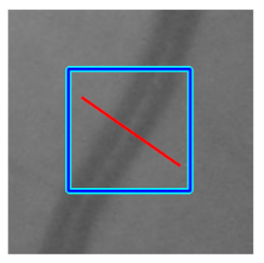
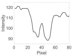
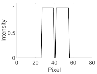
| STEP 5(a): Exclusion Criterion 1 | STEP 5(b): Exclusion Criterion 2 | STEP 5(c): Exclusion Criterion 3 | STEP 5(d): Exclusion Criterion 4 | STEP 5(e): Exclusion Criterion 5 | ||
|---|---|---|---|---|---|---|
| Settings to extract the sum of intensity profiles from interpolated patches | ||||||
| Interpolated Patch | Binary | Gradient | – | – | Binary and gradient | |
| Cross-sectional lines | 5 | 7 | – | – | 7 | |
| 3 pixels | 5 pixels | – | – | 5 pixels | ||
| Orientation | Along main orientation | Perpendicular to main orientation | – | – | Perpendicular to main orientation | |
| Details of exclusion criteria | ||||||
| Input | Sum of intensity profiles from binary interpolated patch | Sum of intensity profiles from gradient interpolated patch | Valley with maximum depth from STEP 5(b) | Valley with maximum depth and global minimum from STEP 5(c) | Sums of intensity profiles from binary and gradient interpolated patches | |
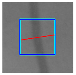
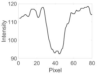
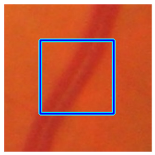
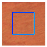
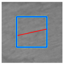
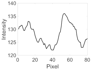
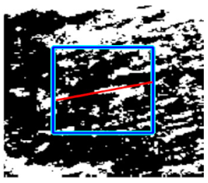
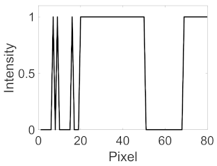
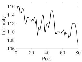
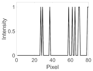
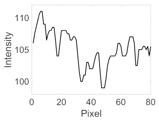
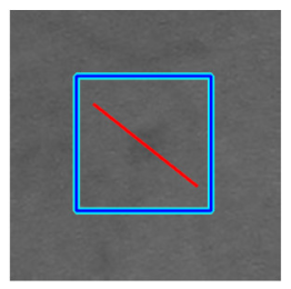
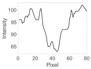
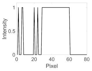
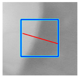
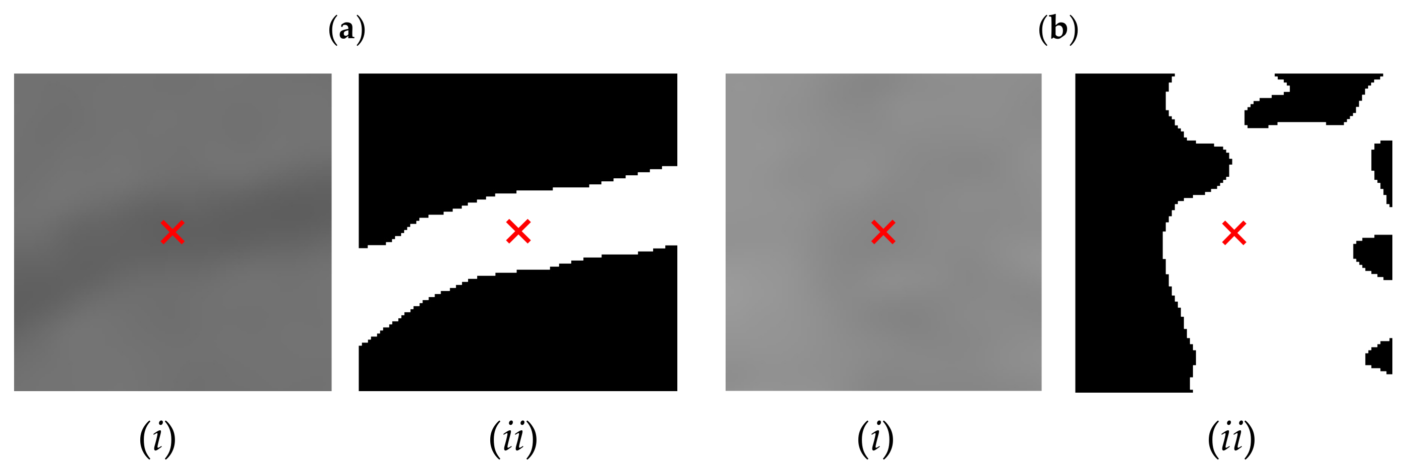
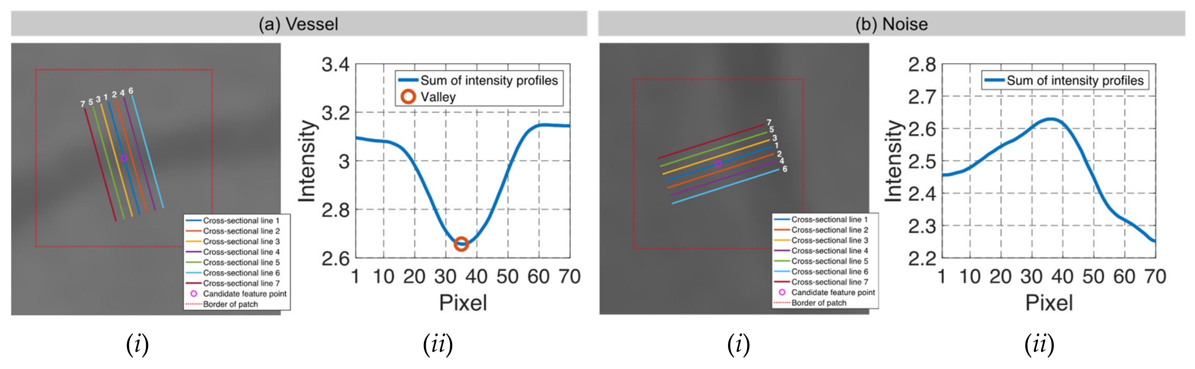
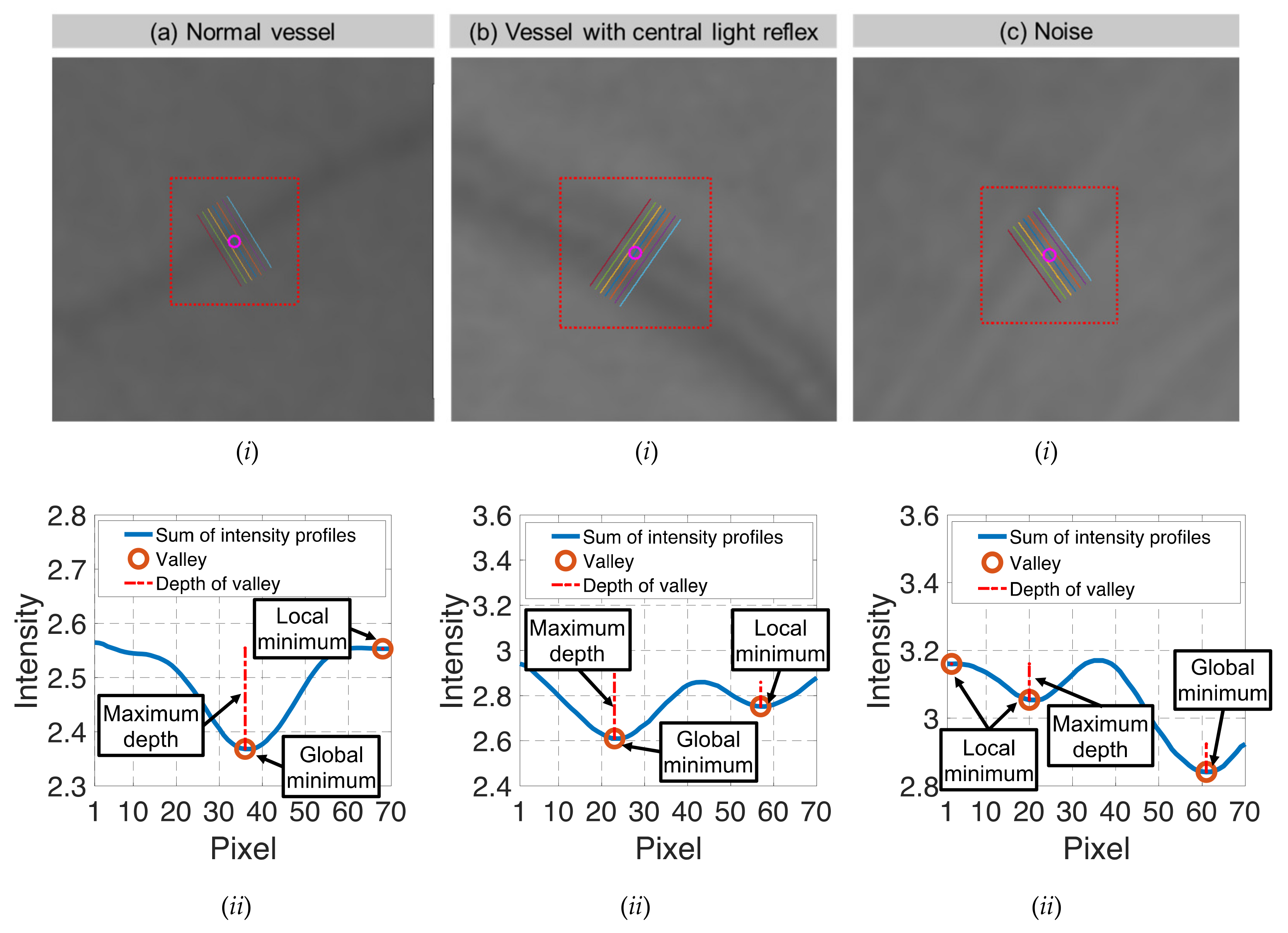
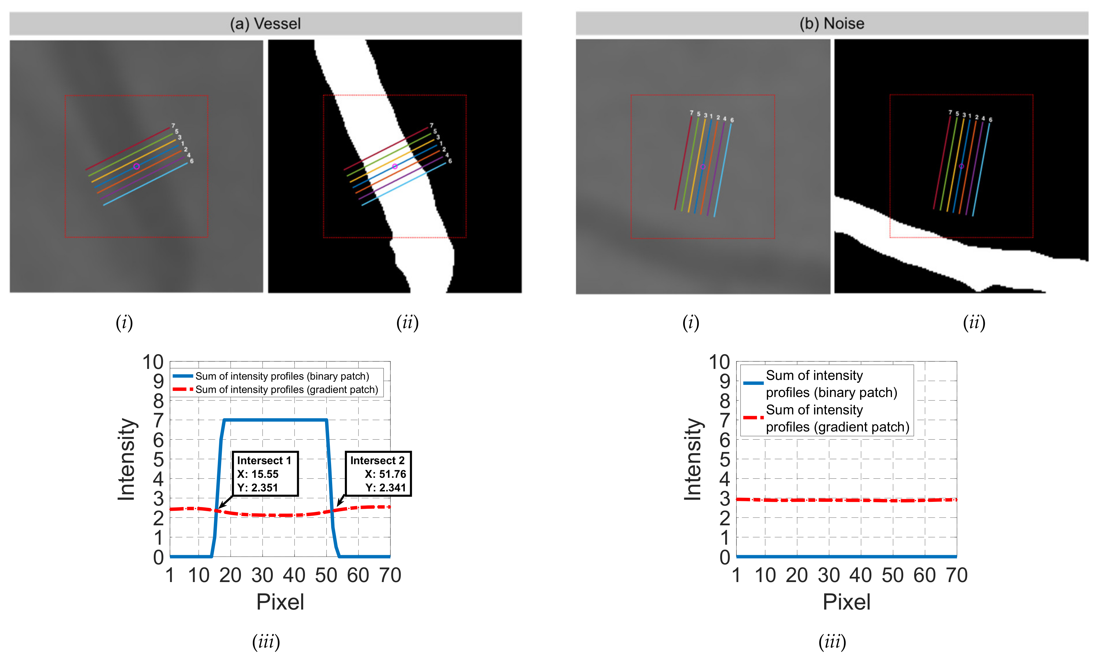
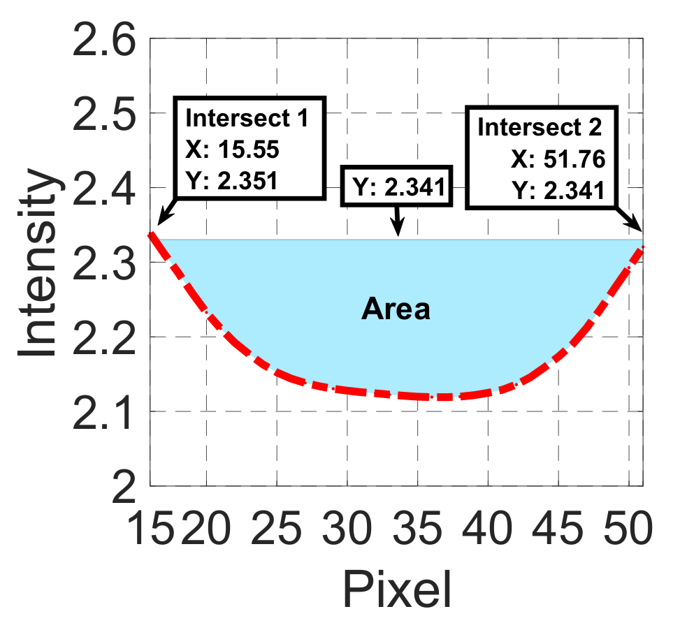
| Candidate feature point | On Vessels | A horizontal line. Figure 7(aii) | With at least a valley. Figure 8(aii) | Is global minimum. Figure 9(aii,bii) | -axis. Figure 10a,b | Intersected when overlaid. Figure 11(aiii) |
| On Noise | With at least a peak. Figure 7(bii) | Without valley. Figure 8(bii) | Is local minimum. Figure 9(cii) | At 1st or 4th section on -axis. Figure 10c | Apart from each other when overlaid. Figure 11(biii) | |
| Descriptions | Datasets | |||
|---|---|---|---|---|
| CHASE_DB1 | DRIVE | HRF | STARE | |
| Total images | 28 | 40 | 45 | 20 |
| Image size (pixels) | 999 × 960 | 564 × 584 | 3504 × 2336 | 605 × 700 |
| Total patients | 14 | 40 | 45 | 20 |
| Age (Years) | 9–10 | 25–90 | N/A | N/A |
| Pathological cases | Vessel tortuosity | 33 images without sign of diabetic retinopathy 7 images with mild early diabetic retinopathy | 15 images of healthy patients 15 images of diabetic retinopathy 15 images of glaucomatous | Abnormalities that obscure the blood vessel appearance, such as hemorrhaging, etc. |
| Field of view | 30° | 45° | 45° | 35° |
| Year | 2012 | 2004 | 2009 | 2000 |
| Ground truth images | 56 | 60 | 45 | 40 |
| Intensity distribution 1 | 22.6136 | 49.3307 | 34.9433 | 49.5126 |
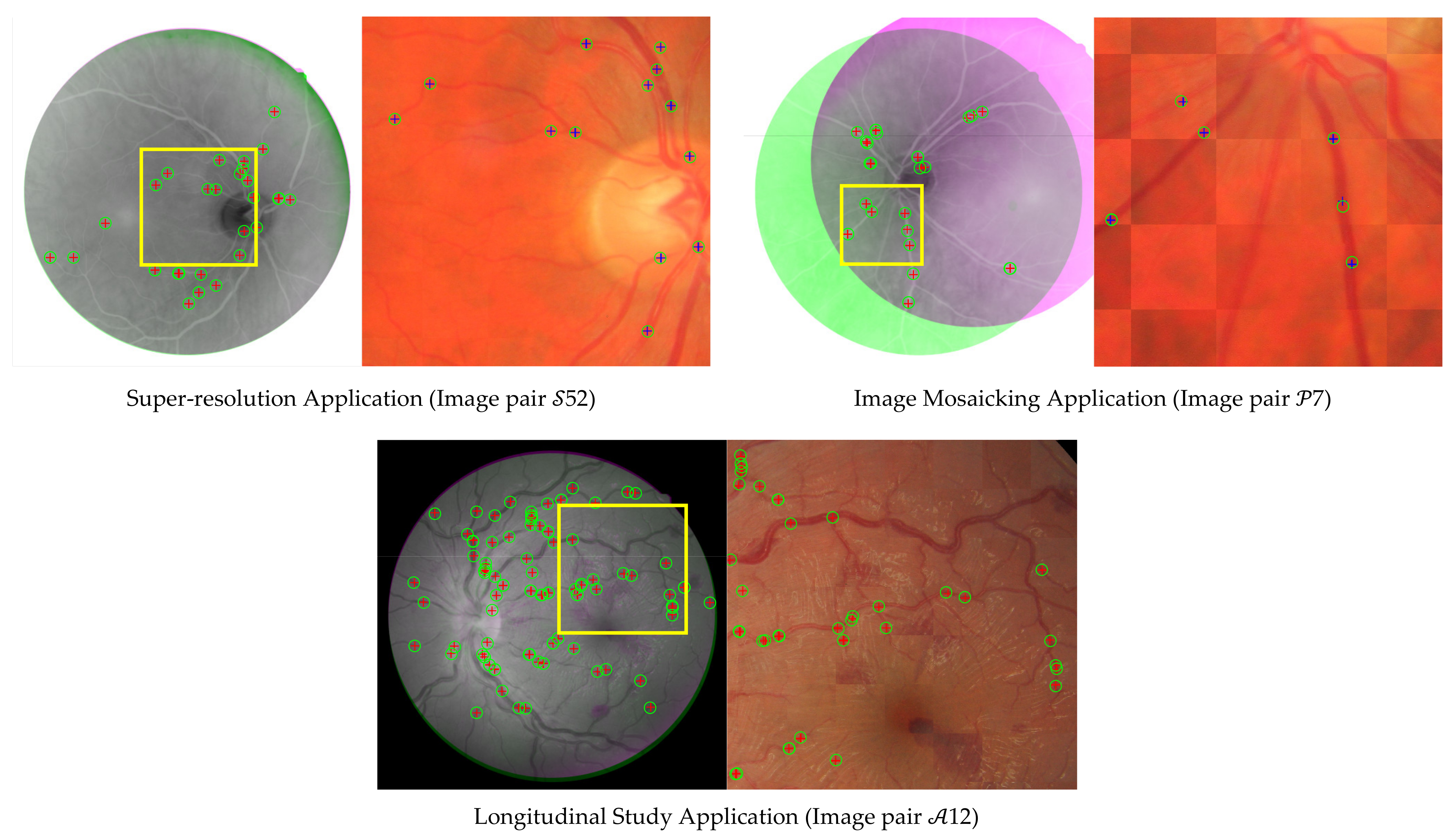
| Descriptions | Retinal Image Registration Applications | ||
|---|---|---|---|
| Super-Resolution | Image Mosaicking | Longitudinal Study | |
| Total images | 71 | 49 | 14 |
| Image size (pixels) | 2912 × 2912 | ||
| Total patients | 39 | ||
| Age (Years) | 19–67 | ||
| Pathological cases | Diabetic retinopathy | ||
| Field of view | 45° | ||
| Year | 2006 to 2015 | ||
| Ground truth images | 10 corresponding points for each image pair | ||
| Anatomical differences 1 | No | No | Yes |
| Scale | ≈1 | ≈1 | ≈1 |
| Overlapping area (%) | 86–100 | 17–89 | 95–100 |
| Rotation (°) | 0°–12° | 6°–52° | 1°–4° |
| Feature Extraction Method | Total Images | Mean | Standard Deviation | Min | Max |
|---|---|---|---|---|---|
| Harris corner | 133 | 41.613 | 21.317 | 0.000 | 92.857 |
| SIFT detector | 133 | 16.164 | 5.411 | 5.241 | 30.299 |
| SURF | 133 | 18.929 | 4.206 | 9.502 | 30.412 |
| Ghassabi’s | 133 | 28.280 | 5.975 | 17.055 | 44.197 |
| D-Saddle | 133 | 20.509 | 4.791 | 12.221 | 31.273 |
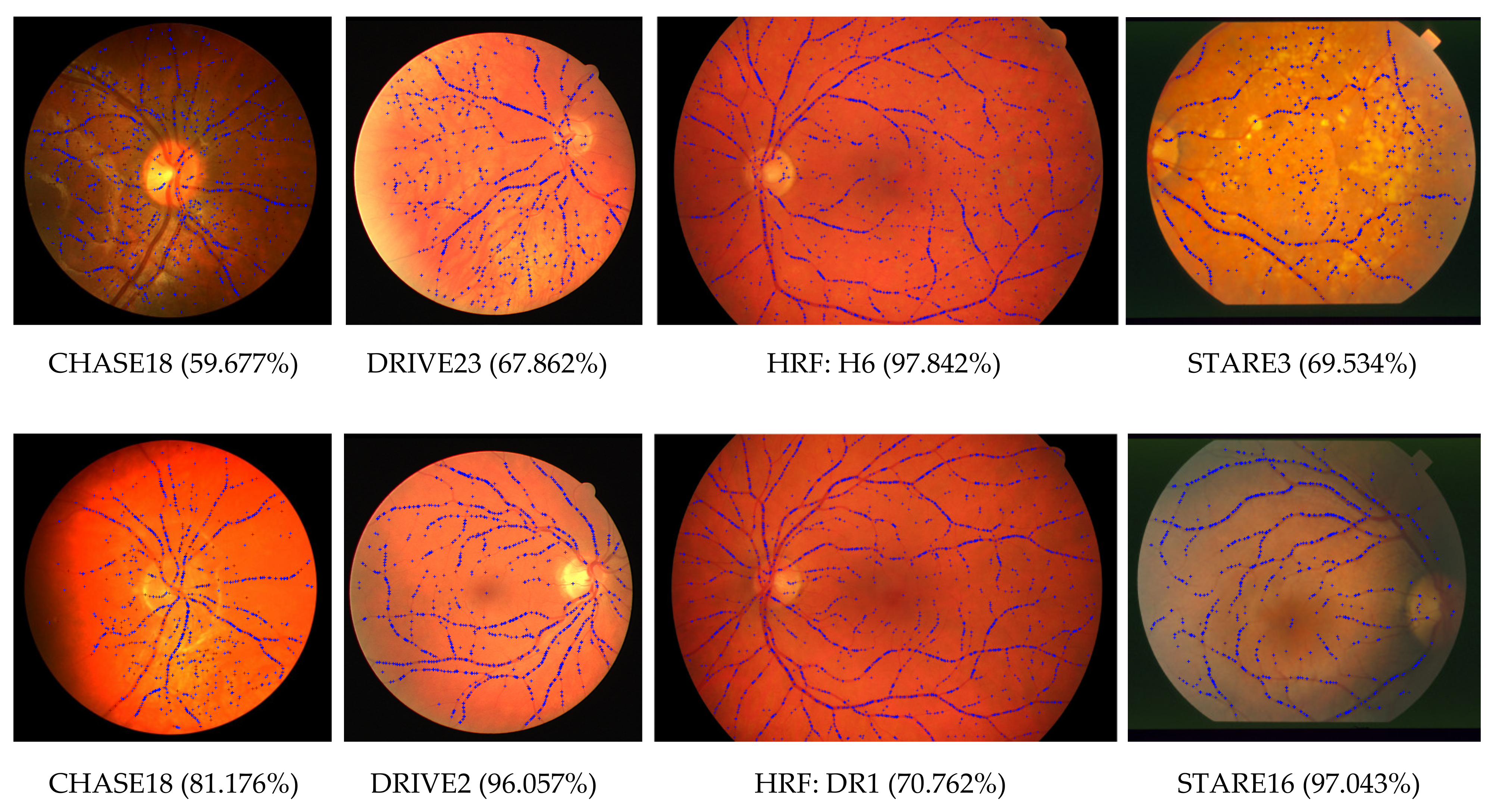
| CURVE | 133 | 86.021 | 9.199 | 59.677 | 97.842 |
| Feature Extraction Method | Image Size | Intensity Distribution | ||
|---|---|---|---|---|
| rs | p-Value | rs | p-Value | |
| Harris corner | −0.178 | 0.041 * | 0.360 | <0.001 ** |
| SIFT detector | −0.649 | <0.001 ** | 0.138 | 0.113 |
| SURF | 0.590 | <0.001 ** | −0.398 | <0.001 ** |
| Ghassabi’s | −0.142 | 0.104 | 0.314 | <0.001 ** |
| D-Saddle | −0.138 | 0.114 | 0.386 | <0.001 ** |
| CURVE | −0.032 | 0.712 | 0.342 | <0.001 ** |
| Feature-Based RIR Technique | Total Image Pairs 1 | Mean | Standard Deviation | TRE (Pixels) | |
|---|---|---|---|---|---|
| Min | Max | ||||
| Overall | |||||
| GDB-ICP | 37 | 27.612 | 44.875 | 2.354 | 10.416 |
| Harris-PIIFD | 5 | 3.731 | 19.024 | 3.319 | 1486.255 |
| Ghassabi’s-SIFT | 17 | 12.687 | 33.407 | 3.082 | 322.616 |
| H-M 16 | 22 | 16.418 | 37.183 | 2.857 | 410.087 |
| H-M 17 | 26 | 19.403 | 39.694 | 2.920 | 60.875 |
| D-Saddle-HOG | 16 | 11.940 | 32.548 | 4.583 | 27.266 |
| CURVE-SIFT | 59 | 44.030 | 49.829 | 1.928 | 1016.330 |
| Super-resolution | |||||
| GDB-ICP | 17 | 23.944 | 42.978 | 0.486 | 4.575 |
| Harris-PIIFD | 2 | 2.817 | 16.663 | 0.785 | 12.850 |
| Ghassabi’s-SIFT | 13 | 18.310 | 38.950 | 0.665 | 15.798 |
| H-M 16 | 18 | 25.352 | 43.812 | 0.554 | 13.903 |
| H-M 17 | 20 | 28.169 | 45.302 | 0.489 | 5.696 |
| D-Saddle-HOG | 10 | 14.085 | 35.034 | 0.748 | 9.327 |
| CURVE-SIFT | 28 | 39.437 | 49.219 | 0.613 | 9.696 |
| Image Mosaicking | |||||
| GDB-ICP | 16 | 32.653 | 47.380 | 1.946 | 6.323 |
| Harris-PIIFD | 0 | 0.000 | 0.000 | 10.041 | 3870.632 |
| Ghassabi’s-SIFT | 0 | 0.000 | 0.000 | 7.358 | 578.494 |
| H-M 16 | 0 | 0.000 | 0.000 | 7.976 | 129.658 |
| H-M 17 | 1 | 2.041 | 14.286 | 3.327 | 41.192 |
| D-Saddle-HOG | 2 | 4.082 | 19.991 | 3.082 | 366.401 |
| CURVE-SIFT | 26 | 53.061 | 50.423 | 1.787 | 19.799 |
| Longitudinal Study | |||||
| GDB-ICP | 4 | 28.571 | 46.881 | 2.354 | 10.416 |
| Harris-PIIFD | 3 | 21.429 | 42.582 | 3.319 | 1486.255 |
| Ghassabi’s-SIFT | 4 | 28.571 | 46.881 | 3.082 | 322.616 |
| H-M 16 | 4 | 28.571 | 46.881 | 2.857 | 410.087 |
| H-M 17 | 5 | 35.714 | 49.725 | 2.920 | 60.875 |
| D-Saddle-HOG | 4 | 28.571 | 46.881 | 4.583 | 27.266 |
| CURVE-SIFT | 5 | 35.714 | 49.725 | 1.928 | 1016.330 |
| Feature-Based RIR Technique | Overlapping Area | Rotation | ||
|---|---|---|---|---|
| rs | p-Value | rs | p-Value | |
| GDB-ICP | 0.443 | <0.001 ** | −0.380 | <0.001 ** |
| Harris-PIIFD | 0.732 | <0.001 ** | −0.723 | <0.001 ** |
| Ghassabi’s-SIFT | 0.795 | <0.001 ** | −0.766 | <0.001 ** |
| H-M 16 | 0.785 | <0.001 ** | −0.763 | <0.001 ** |
| H-M 17 | 0.773 | <0.001 ** | −0.765 | <0.001 ** |
| D-Saddle-HOG | 0.769 | <0.001 ** | −0.745 | <0.001 ** |
| CURVE-SIFT | 0.415 | <0.001 ** | −0.382 | <0.001 ** |
Publisher’s Note: MDPI stays neutral with regard to jurisdictional claims in published maps and institutional affiliations. |
© 2021 by the authors. Licensee MDPI, Basel, Switzerland. This article is an open access article distributed under the terms and conditions of the Creative Commons Attribution (CC BY) license (https://creativecommons.org/licenses/by/4.0/).
Share and Cite
Ramli, R.; Hasikin, K.; Idris, M.Y.I.; A. Karim, N.K.; Wahab, A.W.A. Fundus Image Registration Technique Based on Local Feature of Retinal Vessels. Appl. Sci. 2021, 11, 11201. https://doi.org/10.3390/app112311201
Ramli R, Hasikin K, Idris MYI, A. Karim NK, Wahab AWA. Fundus Image Registration Technique Based on Local Feature of Retinal Vessels. Applied Sciences. 2021; 11(23):11201. https://doi.org/10.3390/app112311201
Chicago/Turabian StyleRamli, Roziana, Khairunnisa Hasikin, Mohd Yamani Idna Idris, Noor Khairiah A. Karim, and Ainuddin Wahid Abdul Wahab. 2021. "Fundus Image Registration Technique Based on Local Feature of Retinal Vessels" Applied Sciences 11, no. 23: 11201. https://doi.org/10.3390/app112311201
APA StyleRamli, R., Hasikin, K., Idris, M. Y. I., A. Karim, N. K., & Wahab, A. W. A. (2021). Fundus Image Registration Technique Based on Local Feature of Retinal Vessels. Applied Sciences, 11(23), 11201. https://doi.org/10.3390/app112311201