
Graph Theory-Based Characterization and Classification of Household Photovoltaics


Abstract
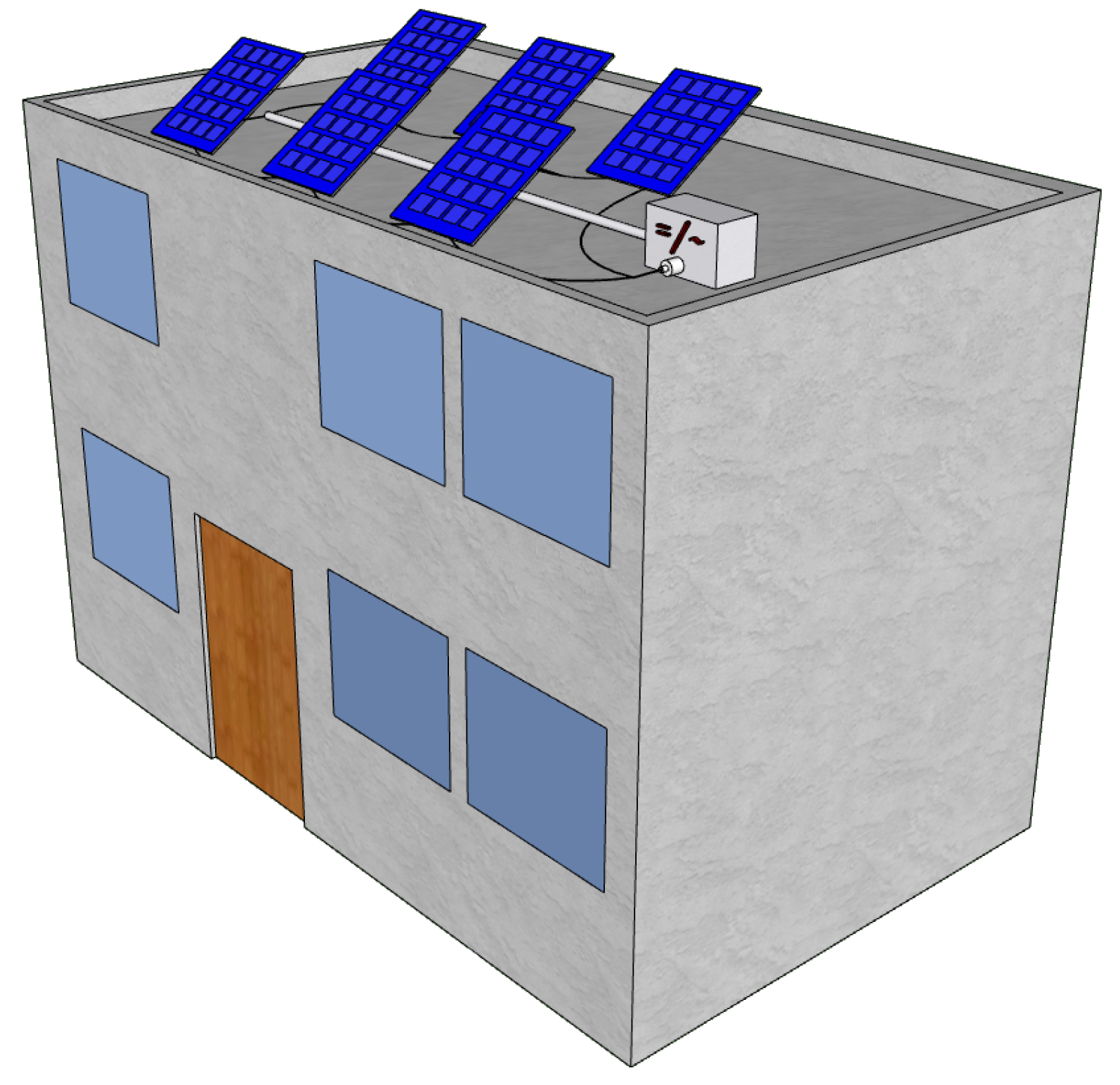
:1. Introduction
2. Graph Theory Background
- (1)
- The number of vertices is known as the order of the graph. The number of edges and/or arcs is known as the size of the graph.
- (2)
- If u and v are vertices of graph G () we write to represent the edge and we say that u is adjacent to v or vice-versa. If u and v are vertices of digraph D we write to represent the arc , and we say that u is adjacent to v, or v is adjacent from u.
- (3)
- The underlying graph U of a digraph D is the one obtained when arcs are replaced by edges .
- (4)
- Given a graph G and , the degree of u written is the number of vertices adjacent to (or from) u. Given a digraph D and , the outdegree of u written is the number of vertices adjacent from u and the indegree of u written is the number of vertices adjacent to u.
- (5)
- A graph H is a subgraph of graph G if and . When , H is said to be a spanning subgraph of G.
- (6)
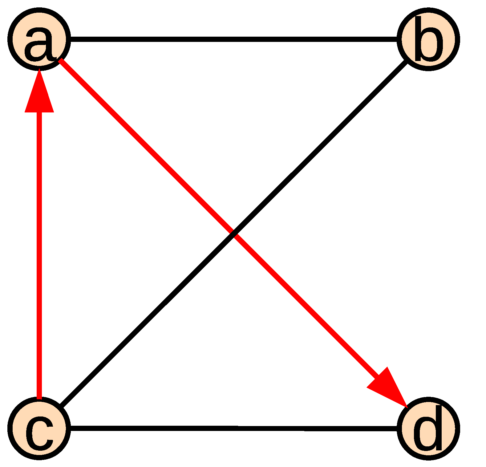
- A path is a graph whose vertices can be labeled by such that its edges are for . A directed path from to is a digraph whose vertices can be labelled by such that its arcs are for .
- (7)
- A graph G is connected if for every given pair of vertices there exists a subgraph P, which is a path starting at u and ending at v. A digraph D is strongly connected if, for every given pair of vertices , there exists a subdigraph P, which is a directed path from u to v. A digraph is weakly connected if its underlying graph is connected.
- (8)
- Two graphs and are isomorphic if there exists a bijective function such that if then . Function is called isomorphism from to .
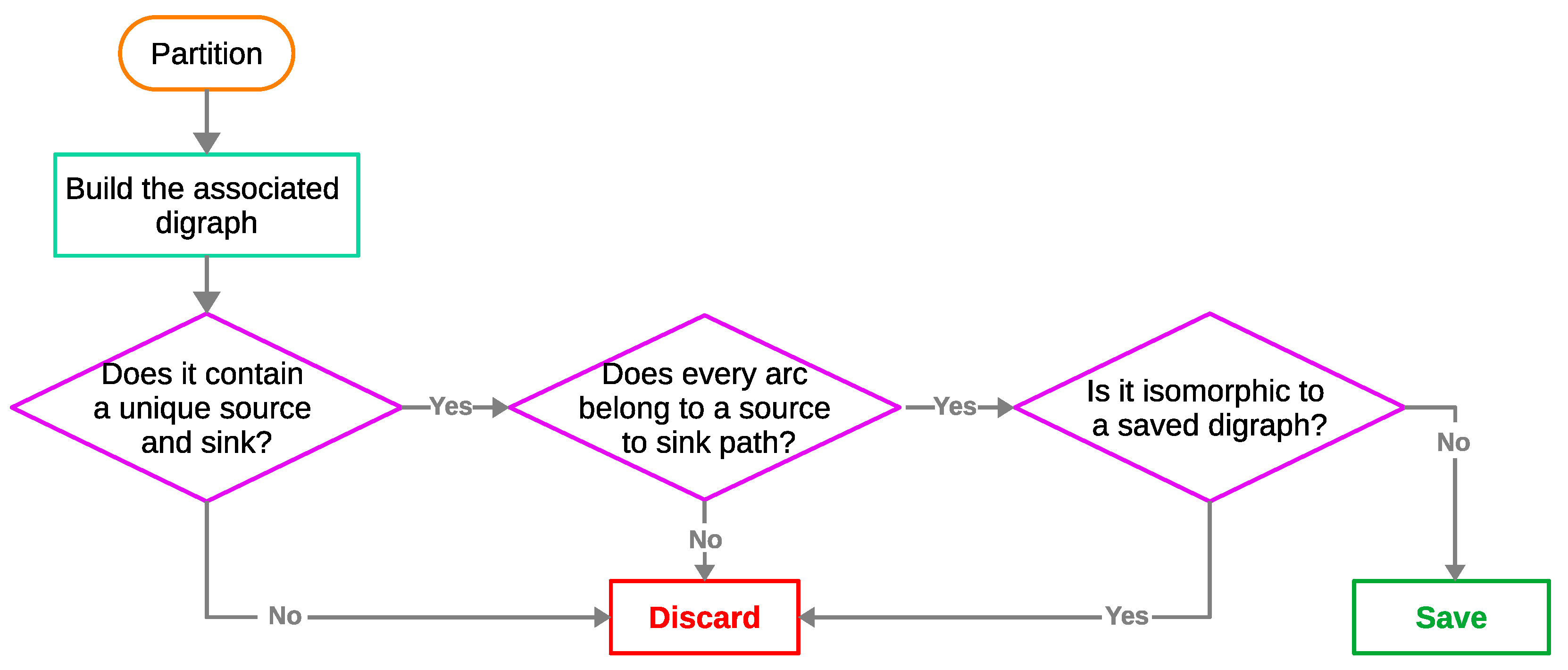
3. Methodology
3.1. Modeling
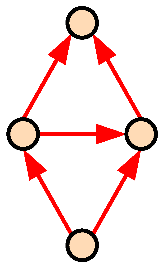
- Panels are represented by arcs, which point in the direction that the photo-current is created. This characterization shows the fact that panels have a determined polarity. The head represents the positive pole and the tail the negative one.
- Vertices represent nodes in the network structure. If different panel poles represented by heads or tails of arcs are incident to or from a given vertex, there exists a cable connection between them.
- (1)
- There exists only one vertex , called the source, such that , i.e., there is only one vertex s, such that there is no arc adjacent to s.
- (2)
- There exists only one vertex , called the target, such that , i.e., there is only one vertex t, such that there is no arc adjacent from t.
- (3)
- For every arc there exists at least one path C from s to t, such that , i.e., every arc in the digraph belongs to a path from s to t.
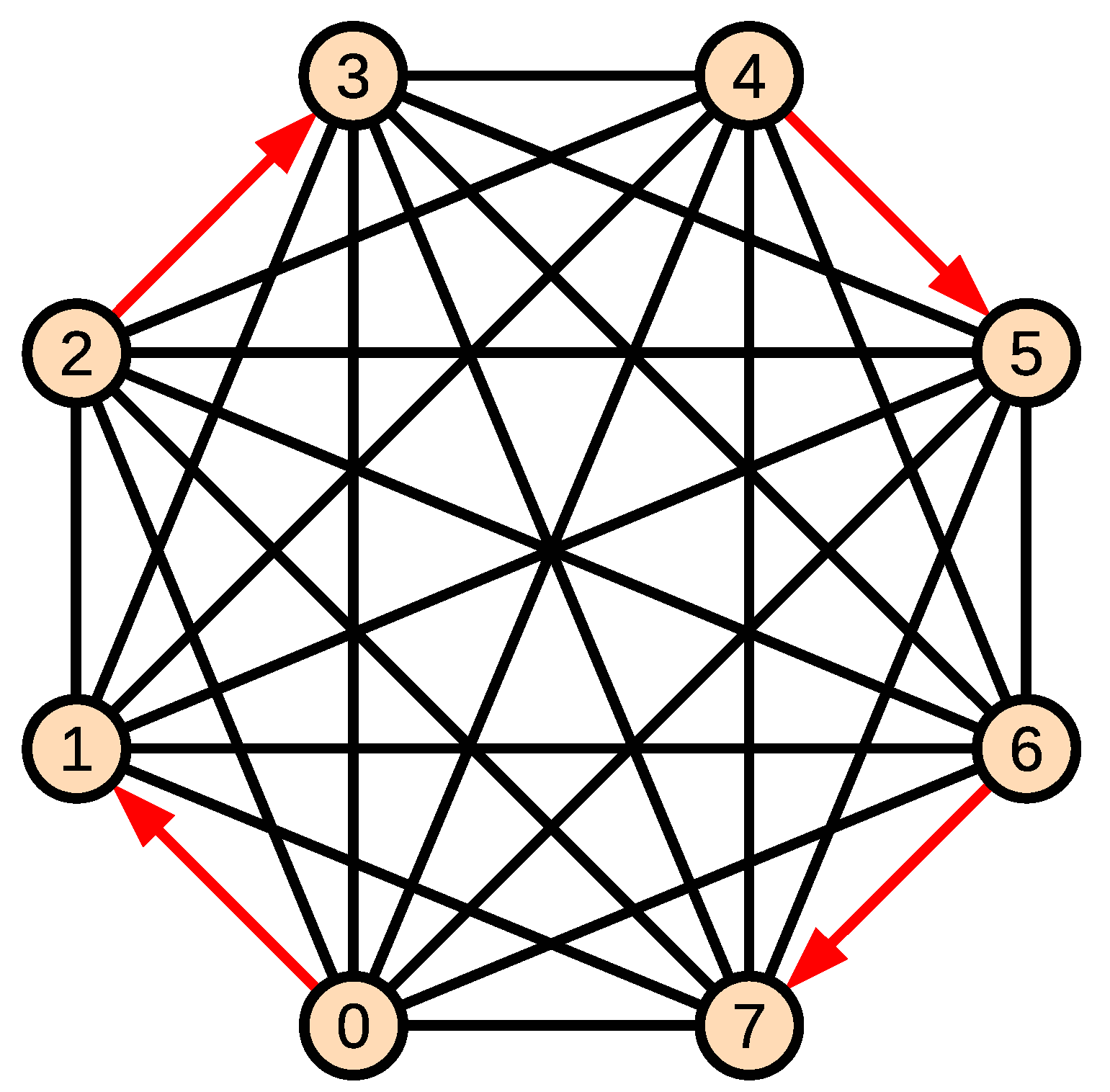
3.2. Construction
- (1)
- Vertex is adjacent to through an arc , and adjacent to all other vertices through an edge for all .
- (2)
- Vertex is adjacent from through the arc , and adjacent to all other vertices through an edge for all .
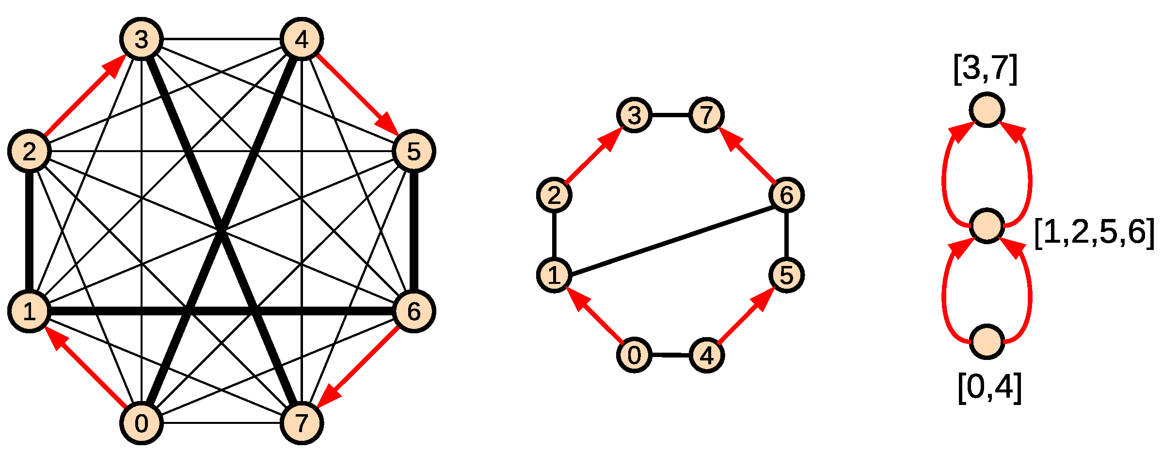
- (1)
- Every vertex is an equivalence class of .
- (2)
- Arc is drawn for every and such that is an arc of H.
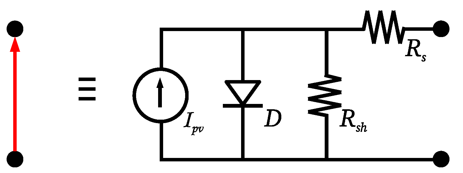
3.3. Simulation
3.4. Reliability
3.5. Expected Value of Power (EVP)
4. Results and Discussion
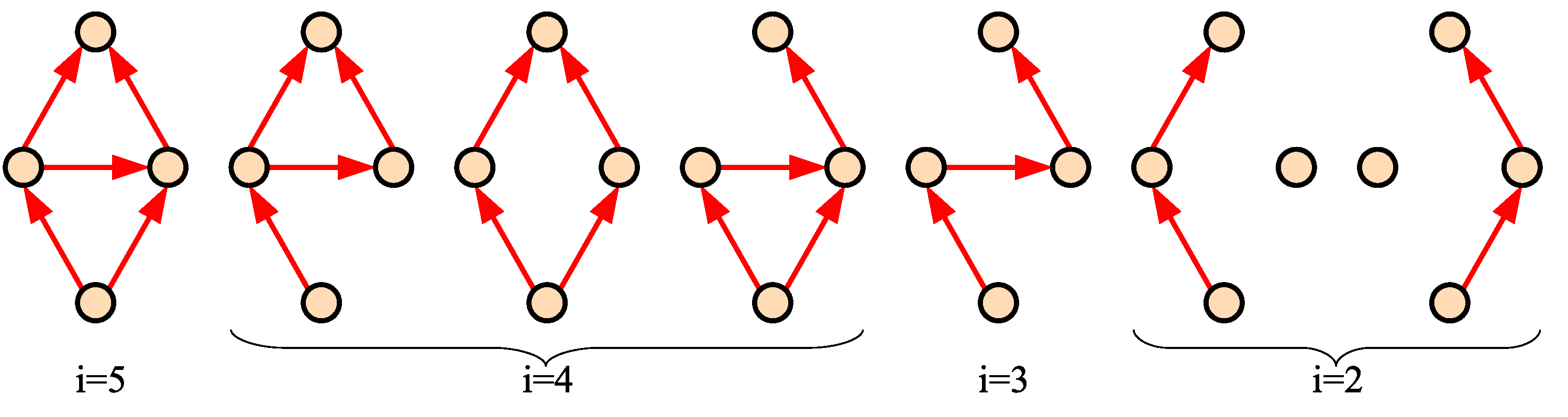
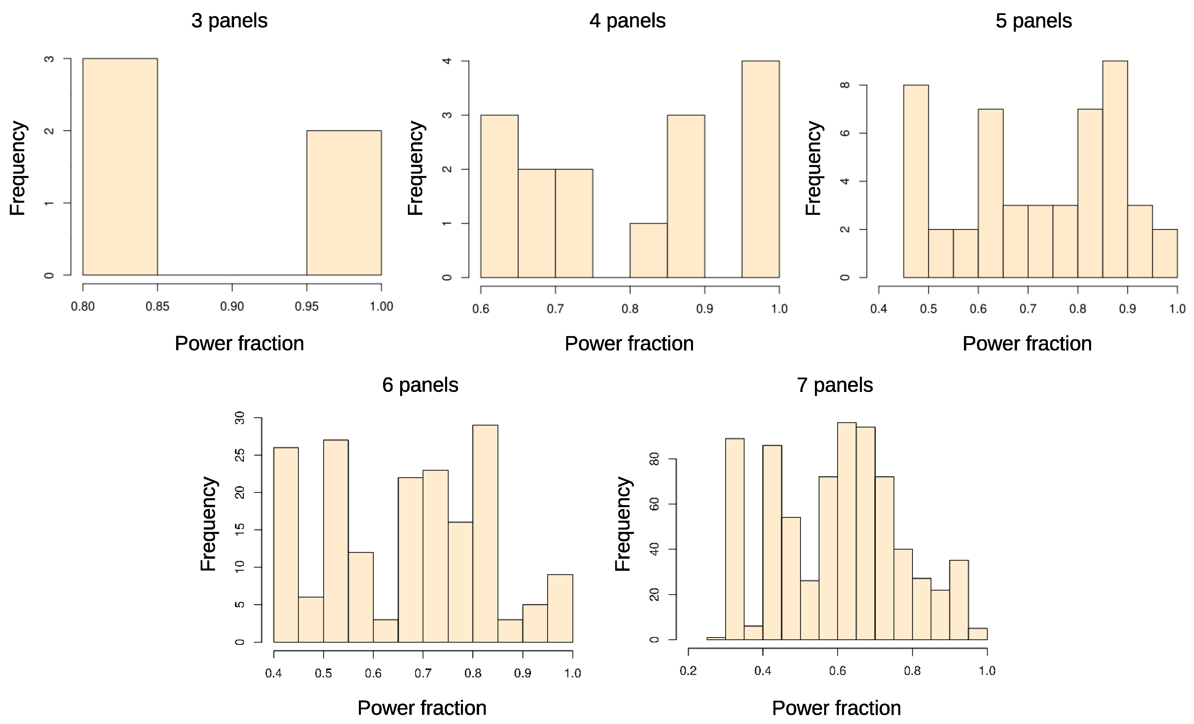
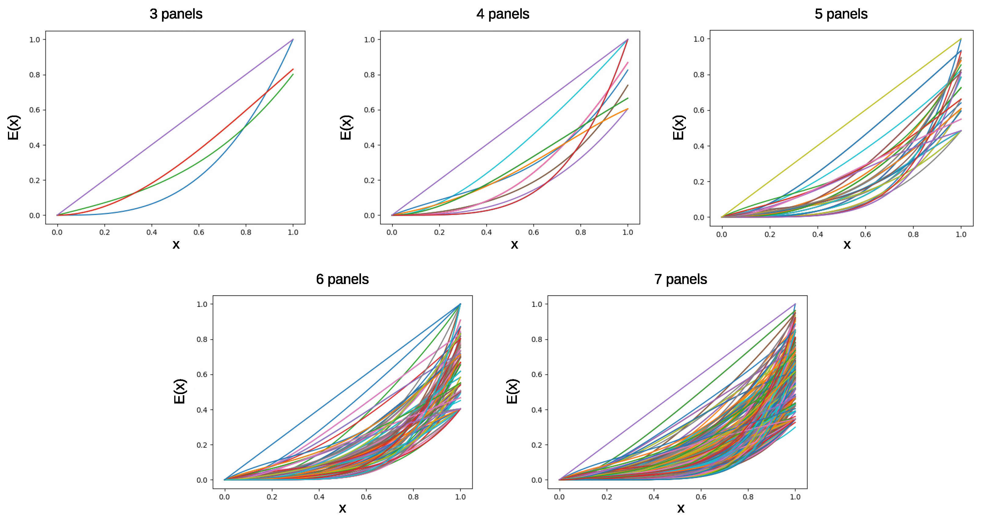
4.1. Construction and Simulation
- (1)
- The number of partitions of elements.
- (2)
- The number of partitions that pass the filter, i.e., that are associated with an array-digraph.
- (3)
- The number of partitions that represent different (non-isomorphic) array-digraphs.
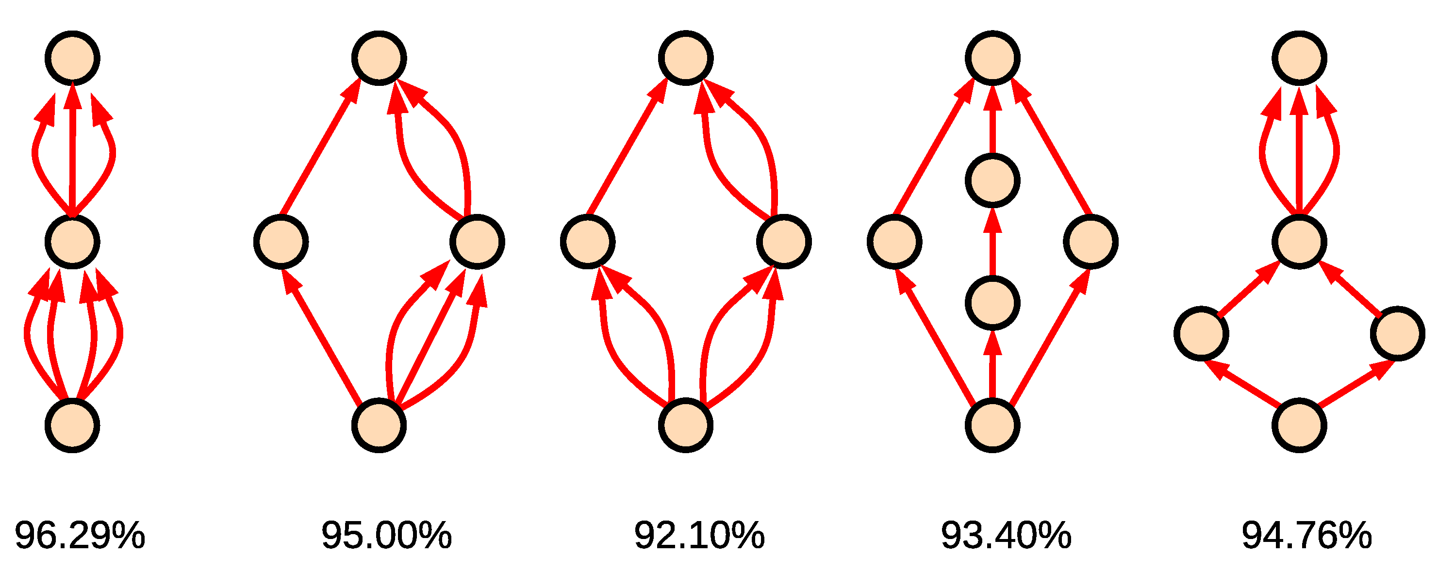
4.2. Reliability
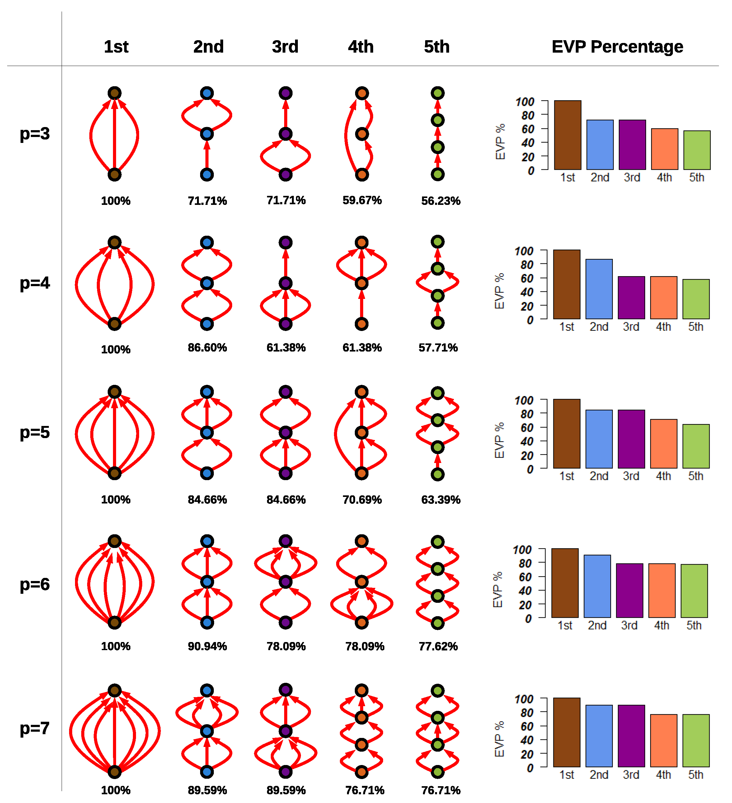
4.3. Expected Value of Power (EVP)
5. Conclusions
Author Contributions
Funding
Informed Consent Statement
Conflicts of Interest
Abbreviations
| PV | PhotoVoltaic |
| GT | Graph Theory |
| ODM | One Diode Model |
| EVP | Expected Value of Power |
References
- Council of European Union. The Energy Performance of Buildings Directive Factsheet. 2019. Available online: https://ec.europa.eu/energy/sites/ener/files/documents/buildings_performance_factsheet.pdf (accessed on 1 November 2021).
- Council of European Union. Council Regulation (EU) No. 844/2018. 2018. Available online: https://eur-lex.europa.eu/legal-content/EN/TXT/PDF/?uri=CELEX:32018L0844&from=EN (accessed on 1 November 2021).
- Council of European Union. European Climate Strategies and Objectives for 2030. 2019. Available online: https://ec.europa.eu/clima/policies/strategies/2030_en (accessed on 1 November 2021).
- Nayak, P.; Mahesh, S.; Snaith, H.; Cahen, D. Photovoltaic solar cell technologies: Analysing the state of the art. Nat. Rev. Mater. 2019, 4, 269–285. [Google Scholar] [CrossRef]
- Sabiha, M.; Saidur, R.; Mekhilef, S.; Mahian, O. Progress and latest developments of evacuated tube solar collectors. Renew. Sustain. Energy Rev. 2015, 51, 1038–1054. [Google Scholar] [CrossRef]
- Usman, M.; Ali, M.; ur Rashid, T.; Ali, H.M.; Frey, G. Towards zero energy solar households—A model-based simulation and optimization analysis for a humid subtropical climate. Sustain. Energy Technol. Assess. 2021, 48, 101574. [Google Scholar] [CrossRef]
- Haegel, N.; Atwater, H.J.; Barnes, T.; Breyer, C.; Burrell, A.; Chiang, Y.M.; De Wolf, S.; Dimmler, B.; Feldman, D.; Glunz, S.; et al. Terawatt-scale photovoltaics: Transform global energy Improving costs and scale reflect looming opportunities. Science 2019, 364, 836–838. [Google Scholar] [CrossRef] [Green Version]
- Obane, H.; Okajima, K.; Ozeki, T.; Yamada, T.; Ishi, T. Minimizing mismatch loss in BIPV system by reconnection. In Proceedings of the 2011 37th IEEE Photovoltaic Specialists Conference, Seattle, WA, USA, 19–24 June 2011; pp. 002406–002411. [Google Scholar] [CrossRef]
- Kour, J.; Shukla, A. Enhanced energy harvesting from rooftop PV array using Block Swap algorithm. Energy Convers. Manag. 2021, 247, 114691. [Google Scholar] [CrossRef]
- Khaleel, N.A.; Mahmood, A.L. Solar Photovoltaic Array Reconfiguration for Reducing Partial Shading Effect. Asian J. Converg. Technol. (AJCT) ISSN-2350 2021, 7, 114–120. [Google Scholar]
- Murillo-Soto, L.D.; Meza, C. Automated Fault Management System in a Photovoltaic Array: A Reconfiguration-Based Approach. Energies 2021, 14, 2397. [Google Scholar] [CrossRef]
- Sugumar, S.; Prince Winston, D.; Pravin, M. A novel on-time partial shading detection technique for electrical reconfiguration in solar PV system. Sol. Energy 2021, 225, 1009–1025. [Google Scholar] [CrossRef]
- Dorfler, F.; Simpson-Porco, J.; Bullo, F. Electrical Networks and Algebraic Graph Theory: Models, Properties, and Applications. Proc. IEEE 2018, 106, 977–1005. [Google Scholar] [CrossRef]
- Islam, M.; Yang, F.; Amin, M. Control and optimisation of networked microgrids: A review. IET Renew. Power Gener. 2021, 15, 1133–1148. [Google Scholar] [CrossRef]
- Atkins, K.; Chen, J.; Kumar, V.; Marathe, A. The structure of electrical networks: A graph theory based analysis. Int. J. Crit. Infrastruct. 2009, 5, 265–284. [Google Scholar] [CrossRef]
- Kanaki, E.; Karazhanov, S. Study of generation-recombination processes by the graph theory. Am. J. Condens. Matter Phys. 2013, 3, 41–79. [Google Scholar]
- Ke, S.; Lin, T.; Chen, R.; Du, H.; Li, S.; Xu, X. A Novel Self-Healing Strategy for Distribution Network with Distributed Generators Considering Uncertain Power-Quality Constraints. Appl. Sci. 2020, 10, 1469. [Google Scholar] [CrossRef] [Green Version]
- Zhao, Y.; Ball, R.; Mosesian, J.; De Palma, J.F.; Lehman, B. Graph-based semi-supervised learning for fault detection and classification in solar photovoltaic arrays. IEEE Trans. Power Electron. 2015, 30, 2848–2858. [Google Scholar] [CrossRef]
- Merino, S.; Sánchez, F.; Sidrach de Cardona, M.; Guzmán, F.; Guzmán, R.; Martínez, J.; Sotorrío, P. Optimization of energy distribution in solar panel array configurations by graphs and Minkowski’s paths. Appl. Math. Comput. 2018, 319, 48–58. [Google Scholar] [CrossRef]
- Iraji, F.; Farjah, E.; Ghanbari, T. Optimisation method to find the best switch set topology for reconfiguration of photovoltaic panels. IET Renew. Power Gener. 2018, 12, 374–379. [Google Scholar] [CrossRef]
- Iraji, F.; Farjah, E.; Ghanbari, T. Method based on graph theory to extract the best switch set for reconfiguration of photovoltaic panels. IET Gener. Transm. Distrib. 2019, 13, 4853–4860. [Google Scholar] [CrossRef]
- Pérez-Rosés, H. Sixty Years of Network Reliability. Math. Comput. Sci. 2018, 12, 275–293. [Google Scholar] [CrossRef]
- Colbourn, C.J. The Combinatorics of Network Reliability; Oxford University Press, Inc.: New York, NY, USA, 1987. [Google Scholar]
- Rana, A.; Thomas, M.; Senroy, N. Reliability evaluation of WAMS using Markov-based graph theory approach. IET Gener. Transm. Distrib. 2017, 11, 2930–2937. [Google Scholar] [CrossRef]
- Xu, Y.; Yu, T.; Yang, B. Reliability assessment of distribution networks through graph theory, topology similarity and statistical analysis. IET Gener. Transm. Distrib. 2019, 13, 37–45. [Google Scholar] [CrossRef]
- Kahouli, O.; Alsaif, H.; Bouteraa, Y.; Ben Ali, N.; Chaabene, M. Power System Reconfiguration in Distribution Network for Improving Reliability Using Genetic Algorithm and Particle Swarm Optimization. Appl. Sci. 2021, 11, 3092. [Google Scholar] [CrossRef]
- Chartrand, G.; Lesniak, L.; Zhang, P. Graphs & Digraphs, 6th ed.; Chapman & Hall/CRC: Boca Raton, FL, USA, 2015. [Google Scholar]
- Yan, J.; Yin, X.C.; Lin, W.; Deng, C.; Zha, H.; Yang, X. A short survey of recent advances in graph matching. In Proceedings of the 2016 ACM on International Conference on Multimedia Retrieval, New York, NY, USA, 6–9 June 2016; pp. 167–174. [Google Scholar] [CrossRef]


| Panels | Num of Partitions | Pass the Filter | Non-Isomorphic |
|---|---|---|---|
| 3 | 203 | 19 | 5 |
| 4 | 4140 | 195 | 15 |
| 5 | 115,975 | 2911 | 49 |
| 6 | 4,213,597 | 59,223 | 181 |
| 7 | 190,899,322 | 1,572,019 | 725 |
Publisher’s Note: MDPI stays neutral with regard to jurisdictional claims in published maps and institutional affiliations. |
© 2021 by the authors. Licensee MDPI, Basel, Switzerland. This article is an open access article distributed under the terms and conditions of the Creative Commons Attribution (CC BY) license (https://creativecommons.org/licenses/by/4.0/).
Share and Cite
Ceresuela, J.M.; Chemisana, D.; López, N. Graph Theory-Based Characterization and Classification of Household Photovoltaics. Appl. Sci. 2021, 11, 10999. https://doi.org/10.3390/app112210999
Ceresuela JM, Chemisana D, López N. Graph Theory-Based Characterization and Classification of Household Photovoltaics. Applied Sciences. 2021; 11(22):10999. https://doi.org/10.3390/app112210999
Chicago/Turabian StyleCeresuela, Jesús M., Daniel Chemisana, and Nacho López. 2021. "Graph Theory-Based Characterization and Classification of Household Photovoltaics" Applied Sciences 11, no. 22: 10999. https://doi.org/10.3390/app112210999
APA StyleCeresuela, J. M., Chemisana, D., & López, N. (2021). Graph Theory-Based Characterization and Classification of Household Photovoltaics. Applied Sciences, 11(22), 10999. https://doi.org/10.3390/app112210999