Comparative Study of Dynamic Stall between an Aircraft Airfoil and a Wind Turbine Airfoil in an Air–Particle Flow

Abstract

Dynamic stall in clean air flow has been well studied, but its exploration in air–particle (air–raindrop or air–sand) flow is still lacking. The aerodynamic performance loss of aircraft (NACA0012) and wind turbine (S809) airfoils and their differences during the hysteresis loop at different pitching parameters are also poorly understood. As shown in this paper, the reduced frequency has little effect on the value of the maximum lift coefficient increment caused by particles, but a larger one can enhance the hysteresis effect and drag the angle of attack, at which the maximum increment is obtained, from the up stroke to the down stroke. The large lift coefficient increments of two airfoils and their difference also have a similar change trend with the reduced frequency. Compared to that of NACA0012 airfoil, the increments of S809 airfoil are obviously greater at three mean angles of attack, especially at 8°, which is the commonly used operating angle. In addition, the angle of attack, at which the maximum lift coefficient is obtained, can be significantly changed by particles in two regions: one is under the effect of deep stall, the other is under the effect of light stall at a low, reduced frequency.

1. Introduction

Dynamic stall, caused by the continuous change of the angle of attack, has a significant effect on aerodynamic performance. It was first discovered in helicopter flow fields, more than fifty years ago [1,2,3,4,5]. They showed that the blade experiences vastly different loads between static and dynamic stall and indicated that the aerodynamic loading is dominated by the intense vortices shed from the vicinity of the wing leading-edge at moderate to high pitching rates. McCroskey et al. [6] further revealed that the initial vorticity of shed vortices is fed from the abrupt, unsteady separation of the turbulent boundary layer, not the laminar bubble. McAlister et al. [7] measured the surface pressure distribution, lift, drag, and pitching moment, and delineated static and dynamic characteristics of eight airfoils both in and out of stall.

Numerical modeling was employed as a new research method and the experimental equipment was also updated. Leishman and Beddoes [8] proposed a semi-empirical dynamic stall model based on the proper consideration of unsteady flow mechanisms. Tuncer et al. [9] numerically studied the unsteady flow fields around airfoils, oscillating in pitch and associated dynamic stall phenomenon. They also presented a numerical method that can be used to calculate the full viscous flow, and the results showed that the formation of the leading-edge vortices can be delayed when the reduced frequency is increased. The means of particle image velocimetry was used in the experiment by Raffel et al. [10], and the result showed the characteristic features of the dynamic stall process, the formation and development of an organized vortex structure, for increasing incidences and the subsequent separation. The comparison between numerical and experimental studies was conducted for four main phases of the dynamic stall process, and the result was encouraging [11]. The computational fluid dynamic successfully captured the three-dimensional dynamic stall [12]. Then, it had a good application in studying the dynamic stall of delta wings. Liu et al. [13,14] implemented a finite, volume-based solver, with a rigid moving mesh and delayed detached eddy simulation (DDES), to analyze the effect of the reduced frequency (RF) on the burst point (BP), helical mode instability, pressure fluctuations, and dynamic pitching stability of a delta and double-delta wings (DW and DDW) in detail. They observed that all the pitching motions postponed the vortex breakdown, and the time-averaged location of the BP has different changes in three sections, divided by a pair of critical RFs, which has been found in several previous experiments. They also indicated, when the upstream speed of the BP is higher than the downstream speed, the variation in the pitching moment is ahead of the AOA, which leads to dynamic instability. Conversely, when the downstream speed is higher than the upstream speed, the DDW is dynamically stable. Yi et al. [15] studied the unsteady aerodynamic characteristics of a 50° sweep delta wing performing pitching oscillations at angle of attack, between 0° and 60°, in numerical and experimental methods. They found that both the lift hysteresis and an unsteady phenomenon of leading-edge vortex evolution were significantly influenced by the pitch rate of the wing. Hu et al. [16] also indicated that the hysteresis effect of lift is magnified with the increasing reduced frequency. The virtual camber effect would dominate the flow field at a sufficiently high reduced frequency, which mitigates the impact of wing geometry on the lift characteristics.

Except on aircrafts, the study of dynamic stall on horizontal axis wind turbines (HAWTs) was also conducted. Butterfield et al. [17] analyzed how dynamic stall varies throughout the blade span of a 10 M HAWT, during yawed and unyawed operating conditions. Shipley et al. [18] provided a statistical representation of dynamic stall occurrence on a downwind HAWT, after analyzing the surface pressure data from the National Renewable Energy Laboratory (NREL). They developed two hypotheses to explain the discrepancy at 30% span and estimated the frequency of dynamic stall on upwind wind turbines. Ramsay et al. [19] conducted a series of steady state and unsteady wind tunnel tests for the S809 airfoil. Ekaterinaris and Platzer [20] addressed some challenging numerical aspects of dynamic stall, such as the prediction of flow reattachment and three-dimensional (3D) effects. Larsen et al. [21] developed a model for aerodynamic lift of wind turbine profiles, based on a backbone curve, in the form of the static lift, as a function of the angle of attack. It combines memory delay effects under attached flow with reduced lift, due to flow separation under dynamic stall conditions. A new prediction technology for dynamic stall, based on the Leishman–Beddoes model, was given by Sheng et al. [22]. In a recent experiment by Pruski and Bowersox [23], they observed the formation and complex evolution of the leading-edge vortex and modified the classical dynamic-stall conceptual model, which is specifically related to the dynamics of the leading-edge vortex. Liu et al. [24] improved the Beddoes–Leishman (B-L) model to account for the characteristics of wind turbine airfoils which have a larger thickness-to-chord ratio compared to aviation airfoils and operate at lower Mach numbers. A series of validations on S809 airfoil are performed to illustrate its advantage.

Martinat et al. [25,26] recommended that the transition model is necessary for accurately predicting dynamic stall at the lower Reynolds number of 10⁵. Both 2D and 3D calculations were carried out, and the results with the SST k-ω model were closer to the experimental data during the up stroke. The 2D RANS simulation is more excellent in capturing significant parts of the coherent large dynamics. Guntur et al. [27] adopted the DDES SST k-ω model, which is combined with the laminar/turbulent transition modeled (the γ-Re_θ model), to present the combined effects of dynamic stall and rotational augmentation in the inboard parts of wind turbine blades. A further investigation was implemented by Zhu et al. [28]; they employed the transition SST model and found that these combined effects can dramatically reduce the sectional lift, drag hysteresis by almost 60% and 80%, and delay the onset of stall, compared to either the rotational augmentation and dynamic stall. Li et al. [29,30] employed the plasma flow to optimize the performance of airfoil dynamic stall in the experiment and numerical calculation, respectively. The large eddy simulation (LES) was well applied in their research. Their results both showed that the strength of the dynamic separation vortex decreases and average aerodynamic force increases under the plasma flow loading. Zhu et al. [31,32] investigated the action of vortex generators under dynamic stall and concluded that the transition SST k-ω model is more suitable for the simulation of dynamic stall, and the vortex generators can elevate the maximum lift coefficient by almost 40%. They also presented comparative analysis of dynamic stall among the 2D airfoil, 3D non-rotating blade, and 3D rotating blade undergoing sinusoidal pitch oscillations. The flow mechanism of three-dimensional dynamic stall is further revealed. In summary, the transition SST k-ω model is crucial to accurately predict the dynamic stall in a highly efficient simulation.

As shown above, the research of dynamic stall on aircrafts and wind turbines in a clean air flow is without interruption since it was discovered. However, the associated exploration in a gas–solid flow is seriously lacking because of the small effect on the aerodynamic performance of an aircraft. He [33] studied the effect of sand particles on the dynamic stall characteristics of NACA0012 airfoil at different particle diameters and concentrations. She preliminarily revealed the changes of airfoil aerodynamic performance, flow structure, and movement characteristics of particles in a gas–solid flow. In her study, it is found that the effect of particles on dynamic stall of NACA 0012 airfoil is small and negligible at a common particle concentration. Guo et al. [34] compared the effect of particles on aerodynamic performance of aircraft wind turbine airfoils. They found when the NACA0012 airfoil runs in a steady air–particle flow, with a particle mass concentration of 1%, lift coefficient penalties are about 0.2% and 1% at the operating angles of attack of the aircraft and the wind turbine, respectively. However, for S809 airfoil, the relative increment of 5.74% is obtained at the operating angle of attack. Therefore, it is significant to study the aerodynamic performance loss of the wind turbine airfoil by particles and the exploration under the effect of dynamic stall is also urgent to be presented. Furthermore, He [33] only focused on the effect of particle characteristics on the hysteresis loop. This paper considers the effect of pitching parameters on hysteresis loops of aircraft and wind turbine airfoils in a gas–solid flow and analyses their difference in different cases.

2. Computational Model

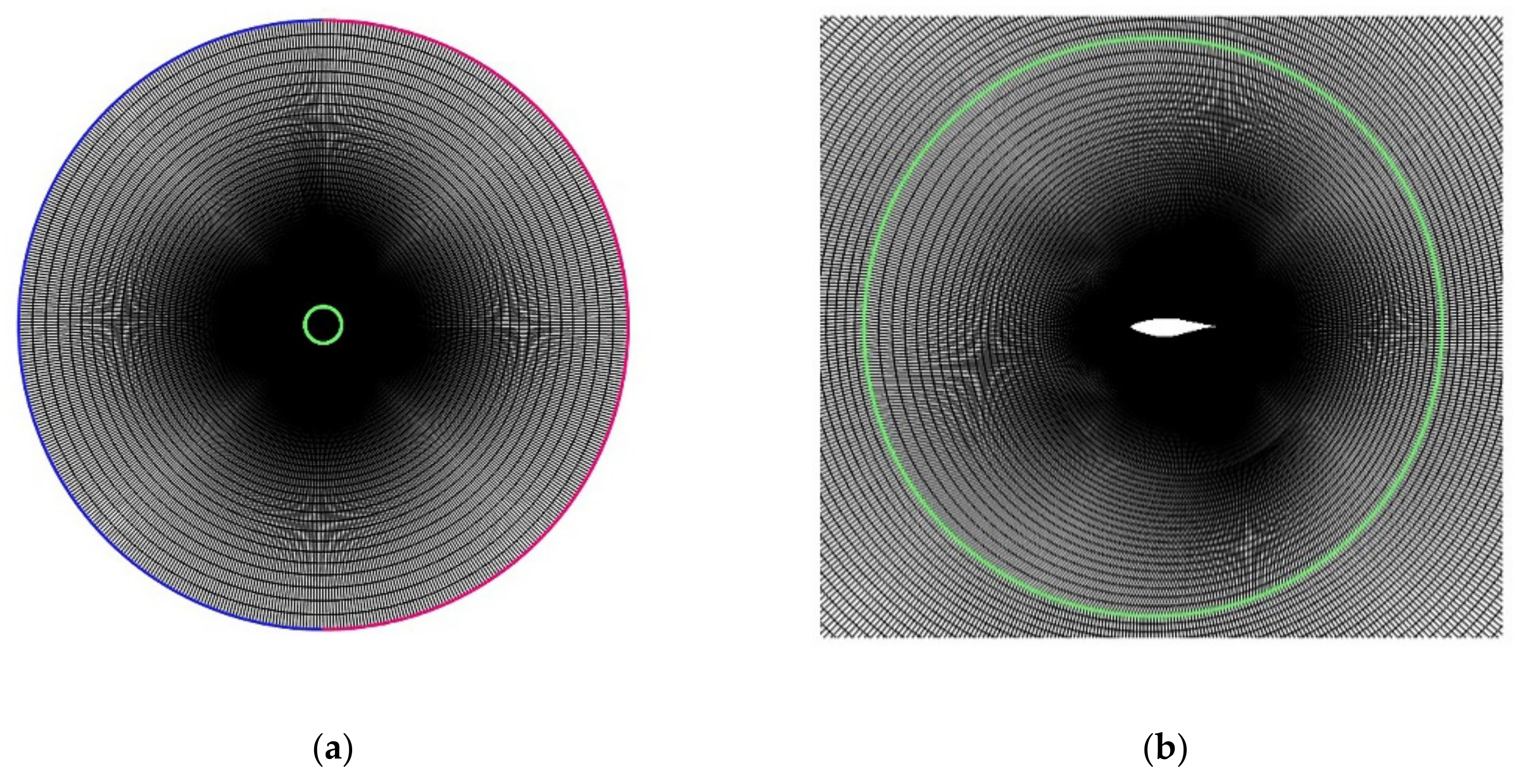
2.1. Numerical Method

The 2D, incompressible URANS equations are solved by ANSYS/FLUENT, for simulating the unsteady flow around a pitching airfoil. The governing equations are written as:

$$\frac{\partial \rho }{\partial t}+\frac{\partial \left(\rho u_i\right)}{\partial x_i}=0$$

(1)

$$\frac{\partial \left(\rho u_i\right)}{\partial t}+\rho u_j\frac{\partial u_i}{\partial x_i}=-\frac{\partial p}{\partial x_i}+\rho \nu {\nabla }^2{u}_i+F_{P,i}$$

(2)

where $x_i$ stands for a coordinate direction, $u_i$ denotes a component of fluid velocity vector, $\rho$, $p$, and $\nu$ are the fluid density, pressure, and kinematic viscosity coefficient, respectively, and $F_{P,i}$ refers to the momentum source term, accounting for the particle effect on the fluid phase.

According to the conclusion by Ekaterinaris and Platzer [20], considering the transition from laminar to turbulent flow is crucial to accurately predict dynamic stall. Therefore, the transition SST model (also known as the γ-Re_θ model) is adopted for turbulence modeling, which couples the SST k-ω eddy viscosity model [35] and two other transport equations [36].

$$\frac{\partial k}{\partial t}+\frac{\partial }{\partial x_j}\left(u_{j}k\right)=\frac{1}{\rho }\frac{\partial }{\partial x_j}\left({\Gamma }_k\frac{\partial k}{\partial x_j}\right)+\frac{G_k-Y_k}{\rho }$$

(3)

$$\frac{\partial \omega }{\partial t}+\frac{\partial }{\partial x_j}\left(u_j\omega \right)=\frac{1}{\rho }\frac{\partial }{\partial x_j}\left({\Gamma }_{\omega }\frac{\partial \omega }{\partial x_j}\right)+\frac{G_{\omega }-Y_k+D_{\omega }}{\rho }$$

(4)

$$\frac{\partial \gamma }{\partial t}+\frac{\partial \left(u_j\gamma \right)}{\partial x_j}=\frac{P_{\gamma 1}-E_{\gamma 1}+P_{\gamma 2}-E_{\gamma 2}}{\rho }+\frac{1}{\rho }\frac{\partial }{\partial x_j}\left[\left(\mu +\frac{{\mu }_t}{{\sigma }_{\gamma }}\right)\frac{\partial \gamma }{\partial x_j}\right]$$

(5)

$$\frac{\partial {\mathrm{Re}}_{\theta t}}{\partial t}+\frac{\partial \left(u_j{\mathrm{Re}}_{\theta t}\right)}{\partial x_j}=\frac{P_{\theta t}}{\rho }+\frac{1}{\rho }\frac{\partial }{\partial x_j}\left[{\sigma }_{\theta t}\left(\mu +{\mu }_t\right)\frac{\partial {\mathrm{Re}}_{\theta t}}{\partial x_j}\right]$$

(6)

The further description of the variables in these four equations can be found in the citied papers. This model has been proven to be reliable in predicting dynamic stall of airfoils [28,31,32,37].

For the simulation of unsteady incompressible flows, the PISO algorithm [38] is suitable, which has been proven by a series of research [28,31,32,37]. In the spatial discretization, the least square cell-based and second-order are employed to compute the gradient and pressure equation. The other convection–diffusion equations are solved with a third-order MUSCL scheme. A second-order implicit scheme is used for time-dependent solution formulation.

The discrete phase model (DPM) is employed to calculate the particle motion. A two-way coupled scheme is adopted, and particles are assumed to be non-interacting, non-deforming, and non-evaporating spheres. Then, the particle trajectories can be solved by:

$$\frac{d{v}_p}{dt}=\beta \left(v_a-v_p\right)+g\left(\frac{{\rho }_p-{\rho }_a}{{\rho }_p}\right)$$

(7)

$$\frac{d{x}_p}{dt}=v_p$$

(8)

where the subscripts $p$ and $a$ denotes the particle and air, $v$ is the velocity vector, $g$ is the acceleration of gravity, $x_p$ is the particle position, and the term $\beta \left(v_a-v_p\right)$ is the drag of per unit particle mass, with $\beta$ being calculated from:

$$\beta =\frac{3\rho C_{D,p}\left|v_a-v_p\right|}{4{\rho }_p{D}_p}$$

(9)

where $D_p$ is the particle diameter and $C_{D,p}$ is the particle drag coefficient, estimated by using the spherical drag law of Morsi and Alexander [39].

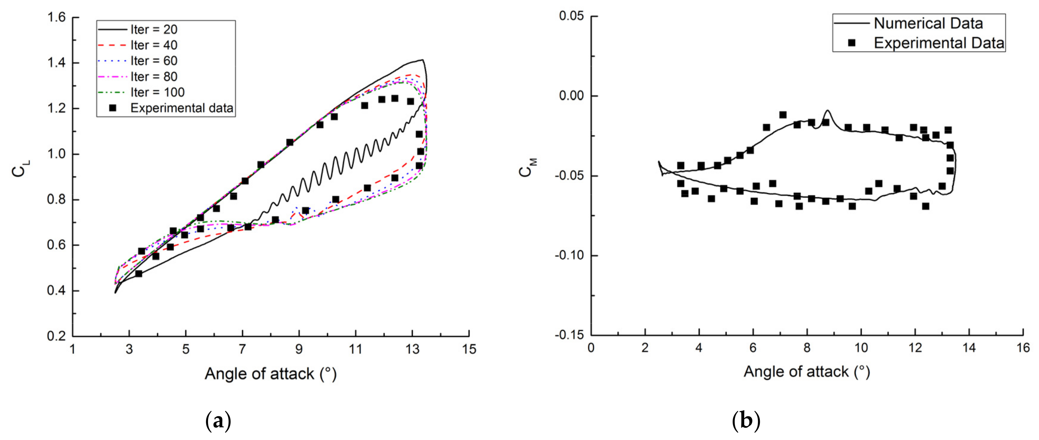
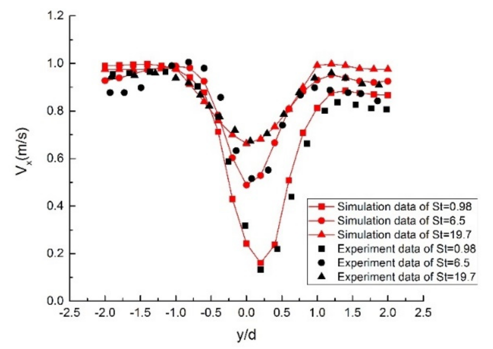
2.2. Numerical Validation

Two airfoils are considered. One is the S809 airfoil, which has the maximum relative thickness of 21%, and the maximum relative camber (of 0.95%) is specifically used in the NREL Phase VI wind turbine. The other is the NACA 0012 airfoil. Figure 1a shows an O-type computational domain with a diameter 50 times as long as the airfoil chord length (c). It contains a smaller circular domain surrounding the airfoil, as shown in Figure 1b, which has a 3c diameter and can rotate around the quarter chord position. After a grid independence study, they, respectively, have the sizes of 553 × 78 and 553 × 199, with a total mesh number of 153,181, which is much larger than that given by Zhu et al. [37]. At least 25 grid cells, in vertical the direction, are used to resolve the boundary layer, and the first cell height is set to make the dimensionless normal distance from wall less than 1.

The pitching motion of the airfoil is defined by:

$$\alpha \left(t\right)={\alpha }_m+{\alpha }_A\sin \left(2\pi ft\right)$$

(10)

where α_m, α_A, and f are the mean angle of attack, the amplitude, and the frequency of oscillation, respectively. The reduced frequency is defined as:

$${\omega }_{red}=\frac{\pi fc}{V_{\infty }}$$

(11)

where V_∞ denotes the free-stream velocity.

A turbulence intensity of 0.1%, which is frequently used in the low turbulence wind-tunnel experiment [40,41], is adopted at the inlet and outlet boundary, and the no-slip condition is used on the airfoil surfaces. The physical time step size is set as 5 × 10⁻⁴ s. The correlation pitching parameters are listed in

Table 1. Correlation pitching parameters of the validation.

Re × 106	αm (°)	αA (°)	f (Hz)	ωred
1.01	8	5.5	1.85	0.077

. Figure 2a shows lift coefficient hysteresis loops of S809 airfoil by numerical and experimental [19] methods in a clean air flow. It was found that the iteration number has great effect on the result, and a number of 80 is an appropriate choice to achieve the balance between accuracy and efficiency. The moment coefficient loop with an iteration number of 80 is shown in Figure 2b, and the good agreement with the experimental result is a further support for the choice.

Figure 3 displays the streamwise velocity distributions of air in the wake of a circular cylinder at three Stokes numbers of 0.98, 6.5, and 19.7. In these three cases, comparisons between numerical results and those from a gas–solid experiment [42] are good, indicating the used DPM is reliable.

3. Results

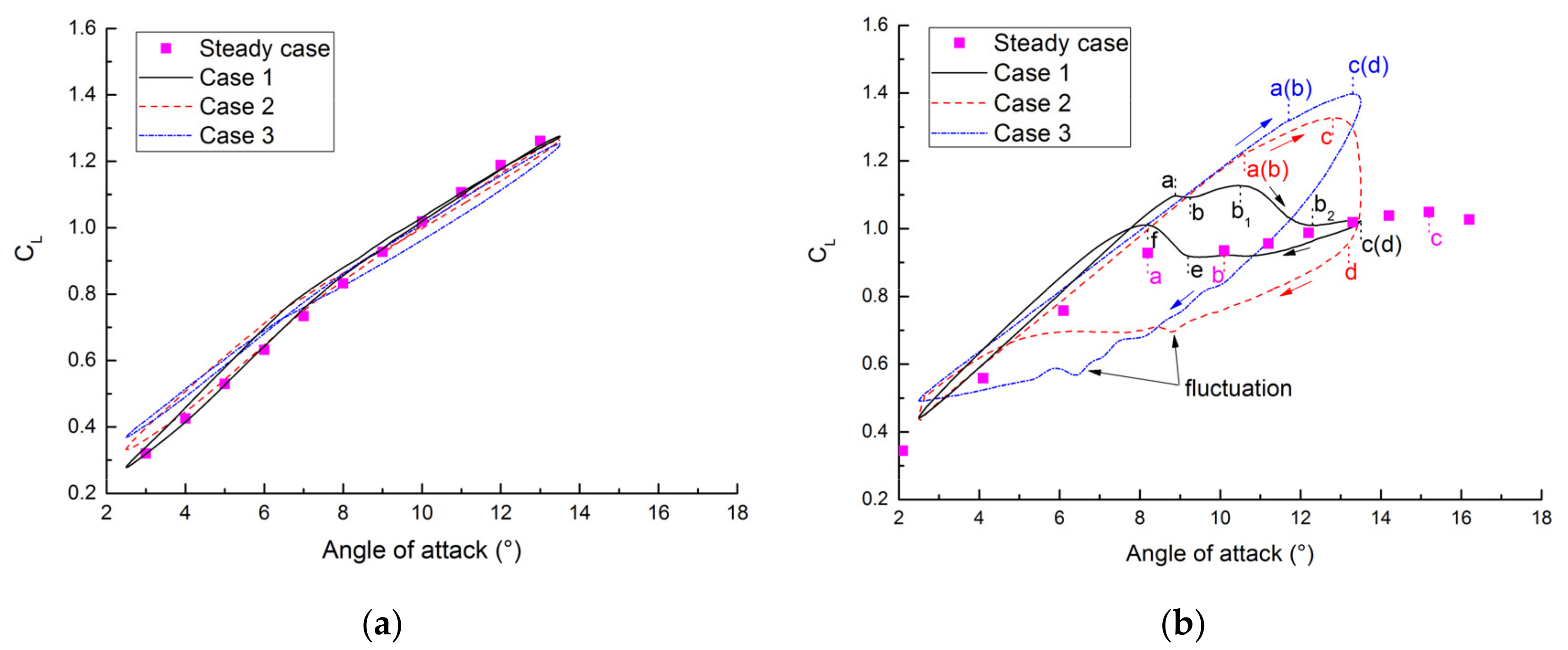
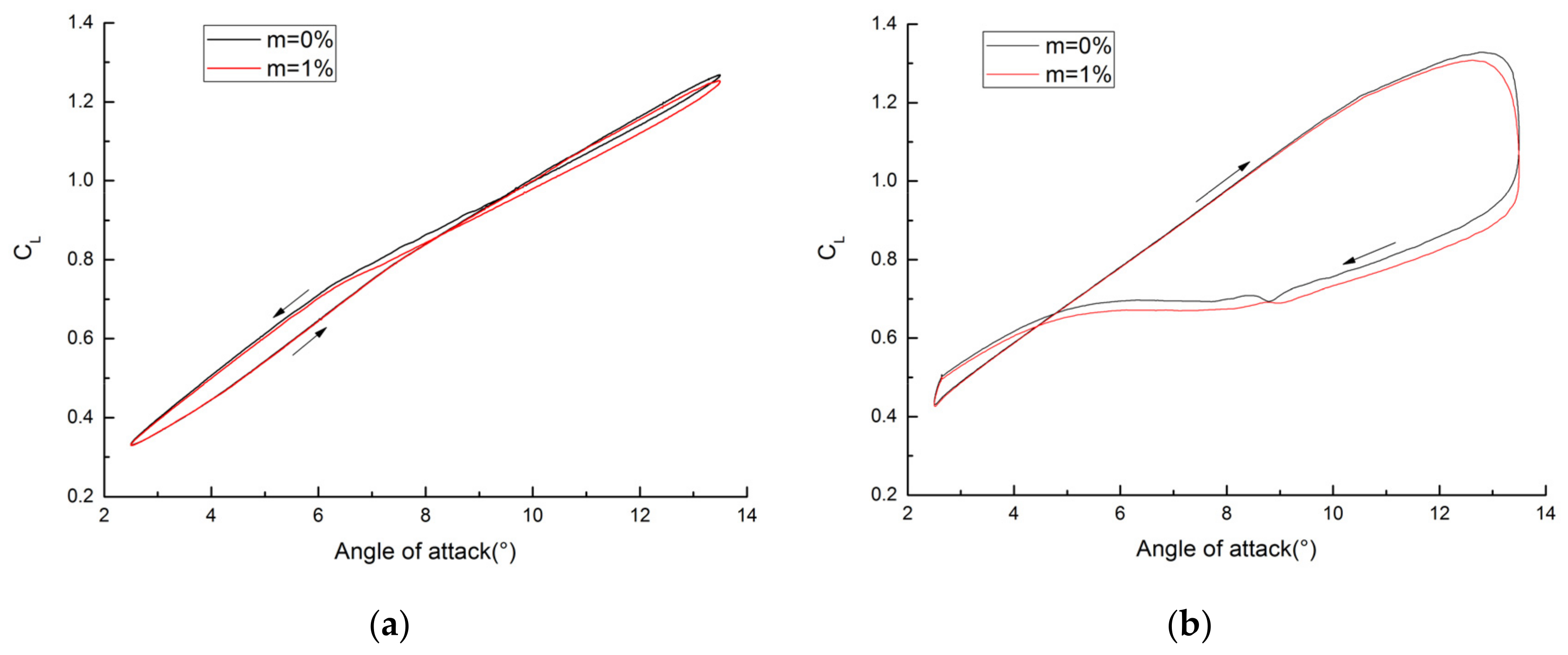
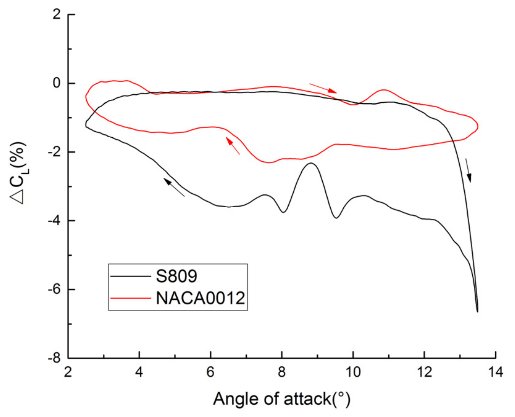
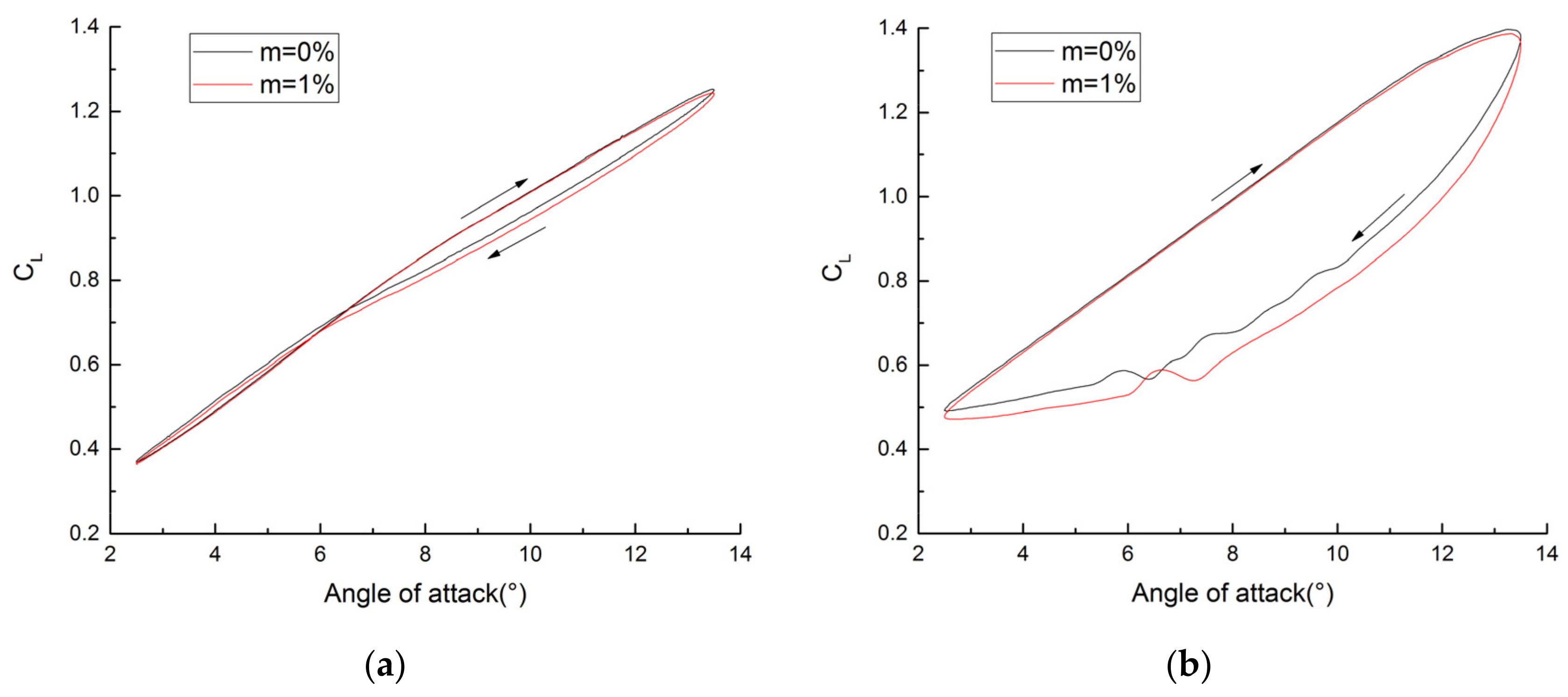
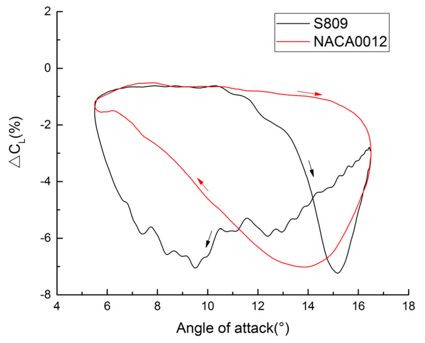
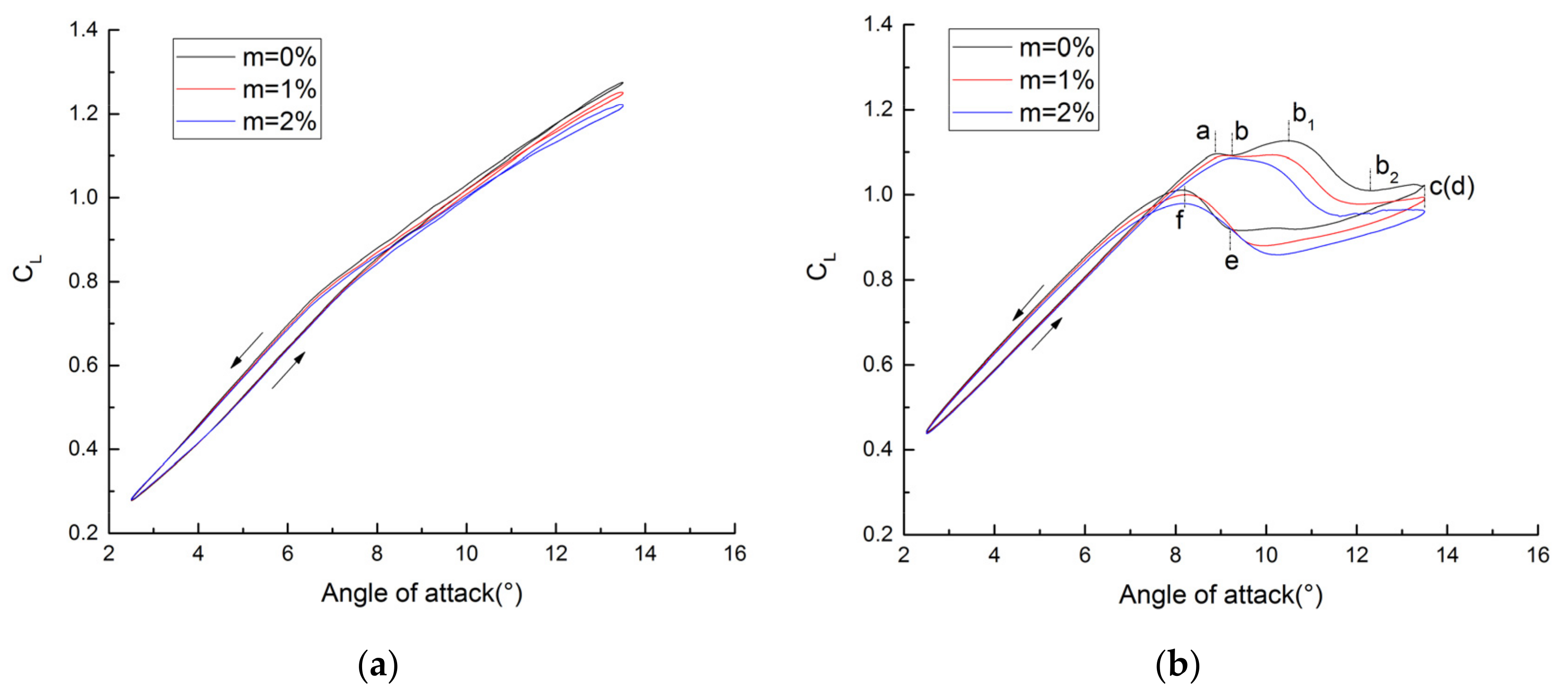
3.1. Hysteresis Loops at Different Reduced Frequencies

In this section, hysteresis loops of the lift coefficient and their difference at three reduced frequencies, listed in

Table 2. The parameters of three pitching cases and their mean computational efficiencies.

Case Number	Stokes Number (St)	Re × 106	αm (°)	αA (°)	f (Hz)	ωred	Mean Computation Time of a Pitching Period in the Air–Particle Flow (hour)
Case 1	0.053	1.01	8	5.5	0.37	0.0154	60
Case 2					1.85	0.0770	15
Case 3					3.33	0.1386	8

, in clean air and air–particle flows are discussed. All cases are computed on a 12-core workstation with a CPU frequency of 3.4 GHz.

Figure 4 shows the hysteresis loops of two airfoils, in four cases, in a clean air flow. For NACA0012 airfoil, the lift coefficient has a linear change with the angle of attack in the steady case, and the values during the up stroke are approximate to those during the down stroke in every pitching case. Three loops also have little difference, except for the inclined angle. However, for S809 airfoil, according to the analysis of the steady case by Guo et al. [34], the lift coefficient stops linearly increasing and decreases slightly near the angle of attack of 8°, due to the forward movement of the boundary-layer separation point from the trailing edge, which is called the light stall. During the following stroke, the lift coefficient increases again and drops into deep stall at an angle greater than 16°. In three pitching cases, the reduced frequency has large effect on the hysteresis loop. The lift coefficients during the up stroke are greatly different from those during the down stroke, which will be discussed as follows, and the mechanisms are also revealed.

In the low reduced frequency case (Case 1), the loop during the up stroke has similar trend with the steady results. As shown in the Figure 4b, the loops are divided into several segments for comparison purposes. Due to the hysteresis effect, a larger range of the linear segment is obtained, and the segment ab has a smaller range than that of the steady case. In segment bb₁, the lift coefficient increases again because of the higher suction peak, which is shown in Figure 5. With the angle of attack increasing, the leading-edge vortex and suction peak barely change, the boundary-layer separation point goes forward rapidly. At the same time, the continuously decreasing pitching speed also cause the lift coefficient to approach the value of the steady case. They both lead to the decrease of the lift coefficient in segment b₁b₂. Then, a similar change to the steady case is presented, until the angle of attack reaches to its maximum value. In the segment de, the lift coefficient keeps close to the steady result because of the slow pitching speed. Notably, the light stall is still effective in this segment. With the further decrease of the angle of attack in segment ef, the airfoil no longer suffers the effect of light stall, the boundary-layer reattaches, and the lift coefficient increases. Finally, the linear change reappears at angles of attack smaller than 8.1°, and the lift coefficients are larger than those during the up stroke.

In the moderate reduced frequency case (Case 2), the linear segment ends up at a larger angle of attack and the segment ab disappears, due to the greater pitching speed. Under the effect of light stall, the lift coefficient in segment ac increases at a smaller speed. Then, in the segment cd, the leading-edge vortex sheds, and the lift coefficient drops sharply, which is defined as deep stall (or full stall). In the following segment, the lift coefficient slowly decreases to the initial value of the up stroke.

In the high reduced frequency case (Case 3), the range of linear segment further increases and the segment ac becomes smaller. There are only two segments during the whole up stroke, and the deep stall also disappears, due to the high pitching speed. That is because the virtual camber effect, which was discussed by Hu et al. [16], starts to dominate the flow field. In addition, the fluctuations in case 2 and 3 are caused by the small number of the inner iteration per step, which is described in Figure 2a. In the following discussion, the fluctuation will become larger, due to the hysteresis effect, especially in the loop of the relative increment between clean air and air–particle cases. Therefore, the mean value is more accurate.

Next, the cases in the air–particle flow are added to the comparison. For the three cases above, increment loops of the lift coefficient of two airfoils, caused by particles, are presented. Figure 6 and Figure 7 display the loops for Case 1 at different particle mass concentrations and the relative increments between concentrations of 0% and 1%, respectively. For NACA0012 airfoil, particles have little effect on the shape of the lift coefficient loop but a decrease for its inclined angle. The flat loop of the relative increment indicates the small loss in aerodynamic performance throughout and its little difference between up and down strokes. The peak value of −2.016% is obtained at the maximum angle of attack. For S809 airfoil, the relative increment loop is also divided into several segments, as well as the discussion in Figure 4b. During the up stroke, particles make the linear segment end up at a larger angle of attack, which increases with the particle concentration. The segment ab is obtained at larger angles of attack; its relative increment decreases first and then increases. In these two segments, the relative increments are both small enough to be out of consideration. Due to the large difference between increments at Point b and Point b₁ by particles, the change of segment bb₁ strongly depends on the particle concentration. It means that the angle of attack, at which the maximum lift coefficient is obtained, has two possibilities. As shown in Figure 6b, the lift coefficient of segment bb₁ increases with the angle of attack at the particle concentration of 0%, and a decrease is presented at the concentration of 2%. The concentration of 1% is the critical value. Then, the maximum lift coefficients at concentrations of 0% and 2% are 1.127 and 1.087, which are obtained at angles of attack of 10.5° (Point b₁) and 9.25° (Point b), respectively. In this segment, the relative increment rapidly increases. In addition, particles make the Point b₁ move to a smaller angle of attack and the larger the concentration, the larger the movement distance and smaller the range of segment bb₁. In the following three segments, the lift coefficient in the air–particle flow is approximately parallel to that in the clean air flow. The relative increment continues to increase, and the maximum value of −6.55% is obtained at the angle of attack of 11.3° in segment b₁b₂. In whole segment b₂c and the first half of segment de, the relative increment is around 3%, and when the angle of attack decreases to 10°, it increases to a peak value of −4.5%. Then, the increment rapidly decreases, until the positive value is obtained. Compared to that in the clean air flow, the Point E appears at a larger angle of attack in the air–particle flow. It means that particles can advance the reattach of the boundary layer. The range of segment ef increases with the particle concentration because the influence of particles at Point e is larger than that at Point f. Due to the hysteresis effect, two loops (m = 0% and 1%) intersect in this segment and a positive peak relative increment of 2.16% is obtained at the angle of 9.06°. Then, it decreases until the negative value is obtained again. Finally, in the linear segment, the relative increment changes in a negligible range, although it is larger than that during the up stroke.

In Figure 8 and Figure 9, for Case 2, particles also have little effect on the loop of NACA0012 airfoil. The angle of attack, where the maximum lift coefficient is obtained, is unchanged, which is different from that of S809 airfoil. During the up stroke, the relative increments of two airfoils are around −0.25%, except in the last section. From 12.5° to 13.5°, they increase to −1.3% and −6.85%, respectively. During the down stroke, the relative increment of NACA0012 airfoil continuously increases and obtains the maximum value of −2.47% at the angle of attack of 7.5°. Then, it keeps a slow decrease until the end. The relative increment of S809 airfoil rapidly decreases first and obtains the value of −3.5% at the angle of attack of about 12°. In the middle section, a fluctuation is shown, and the cause is revealed above. From 6.5° to 2.5°, the relative increment keeps decreasing. Obviously, areas bounded by the two relative increment loops; in Case 2, it is larger than those in Case 1, which illustrates the grater difference of the former between up and down strokes.

In Figure 10 and Figure 11, for Case 3, during the up stroke, relative increments of two airfoils are both smaller than 1% in most sections, except for that of S809 airfoil at angles of attack smaller than 4°. A maximum value of −3.02% is obtained at the minimum angle of attack. During the down stroke, the increment of NACA0012 airfoil has a mean value of −1.9%, and the maximum value of −2.32% is obtained at the angle of 7.6°. For S809 airfoil, the relative increment rapidly increases from −1.37% at 13.5° to −6% at 12.3°. Then, it increases again with a small slope. The maximum value, which is about −7%, appears at a middle angle of attack. In addition, areas bounded by the relative increment loops of two airfoils further increases, and it is greatly obvious for S809 airfoil. Therefore, a larger reduced frequency can increase the range of the large aerodynamic performance loss and the difference between two airfoils, especially during the down stroke.

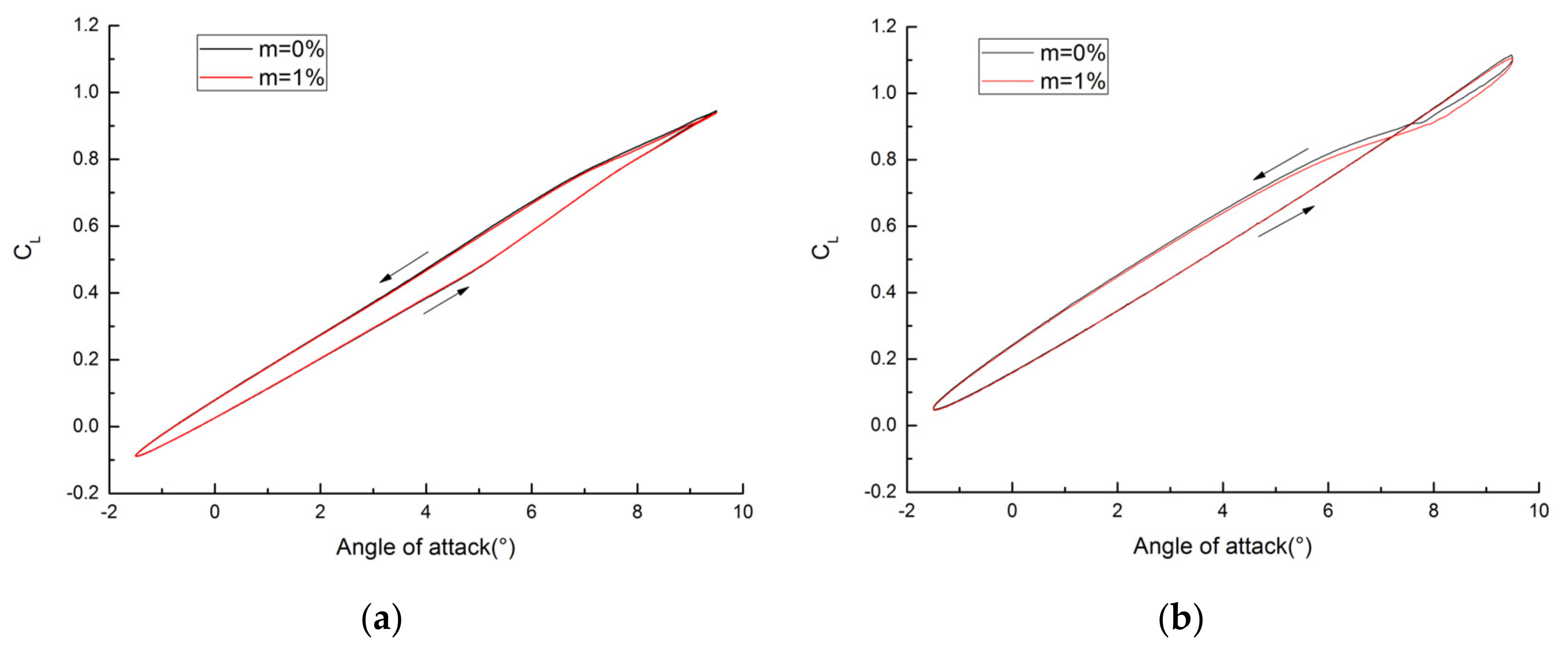
3.2. Hysteresis Loops at Different Mean Angles of Attack

In the previous section, the comparison is presented at a mean angle of attack of 8°. Another two mean angles of attack are adopted to further reveal their difference. The default particle mass concentration is also 1% and the more details are listed in

Table 3. The pitching parameters of three cases.

Case Number	Stokes Number (St)	Re × 106	αm (°)	αA (°)	f (Hz)	ωred
Case 4	0.053	1.01	4	5.5	1.85	0.0770
Case 2			8		1.85	0.0770
Case 5			11		1.85	0.0770

. Then, the computed results of these three cases are discussed, respectively.

In Figure 12a, for Case 4, the loop of NACA0012 airfoil is hardly changed by particles, due to its insensitivity during both up and down strokes. However, in Figure 12b, the loops of S809 airfoil during the beginning of the down stroke have apparently smaller lift coefficients than those during the end of the up stroke, which is caused by the light stall. Although particles have an obvious change in this region, it is still too small to be paid attention to. Therefore, the effect of particles on the lift coefficient is slight and negligible at the default particle mass concentration in the whole loop.

For two airfoils, the angle of attack, at which the maximum lift coefficient is obtained, is unchanged by particles. In order to ascertain this phenomenon, two larger particle mass concentrations of 3% and 5% are adopted, and the results are listed in

Table 4. Angles of attack, at which the maximum lift coefficient is obtained, for Case 4.

Particle Mass Concentration	Maximum Lift Coefficient Angle (°)
	NACA0012	S809
0%	9.5	9.5
1%
3%
5%

. It is found that particles do not change the angle at which the maximum lift coefficient is obtained, even though it is under the effect of light stall at moderate and high reduced frequencies.

The comparison for Case 2 was presented in Figure 8 and Figure 9. In

Table 5. Angles of attack, at which the maximum lift coefficient is obtained, for Case 2.

Particle Mass Concentration	Maximum Lift Coefficient Angle (°)
	NACA0012	S809
0%	13.5	12.8
1%		12.6
3%		12.3
5%		12

, for NACA0012 airfoil, all angles of attack, at which the maximum lift coefficient is obtained, were 13.5°, while for S809 airfoil, the value decreases with the mass concentration. This may illustrate that the angle of attack, at which the maximum lift coefficient angle is obtained, can be changed by particles in the region, which suffers the effect of deep stall.

Finally, as shown in Figure 13 for Case 5, two airfoils both suffer the effect of deep stall and have different degradations of the lift coefficient near the maximum angle of attack. In Figure 14, during the up stroke, the relative increment of NACA0012 airfoil is smaller than −1.25% at angles of attack less than 15° and increases to −3.01% at 16.5°. With the angle of attack decreasing, it increases again at a greater speed rate. Then, the maximum increment of −7.02% is obtained at 13.9°. In the following region, the relative increment linearly decreases until the angle of attack reaches to 6.2°. For S809 airfoil, the relative increment is smaller than −1.5% at angles of attack less than 12° and rapidly increases at following angles of attack. The first peak value of −7.23% appears at 15.2° and it decreases to −3% at 16.5°. During the down stroke, the relative increment increases again, and the second peak value is −7.05% at 9.5°. Then, the decrease runs through the rest region. In brief, particles have large effect on the lift coefficient of both airfoils during the down stroke. However, during the second half of the up stroke, particles also have a large effect on the lift coefficient of S809 airfoil.

Table 6. Angles of attack, at which the maximum lift coefficient is obtained, for Case 5.

Particle Mass Concentration	Maximum Lift Coefficient Angle (°)
	NACA0012	S809
0%	16.2	14.3
1%	16	13.6
3%	15.8	13
5%	15.5	12.4

shows angles of attack, at which the maximum lift coefficient is obtained, of two airfoils at different particle concentrations. They both decrease with the particle mass concentration. In summary, particles can change the angle of attack, at which the maximum lift coefficient is obtained, in the region under the effect of deep stall.

4. Conclusions

This paper shows the comparison of relative increment loops of the lift coefficient caused by particles between an aircraft airfoil (NACA0012) and a wind turbine airfoil (S809) at different reduced frequencies. Then, the differences of relative increment loops of the lift coefficient between two airfoils at three mean angles of attack are also discussed. Three important conclusions can be reached as follows:

(1)

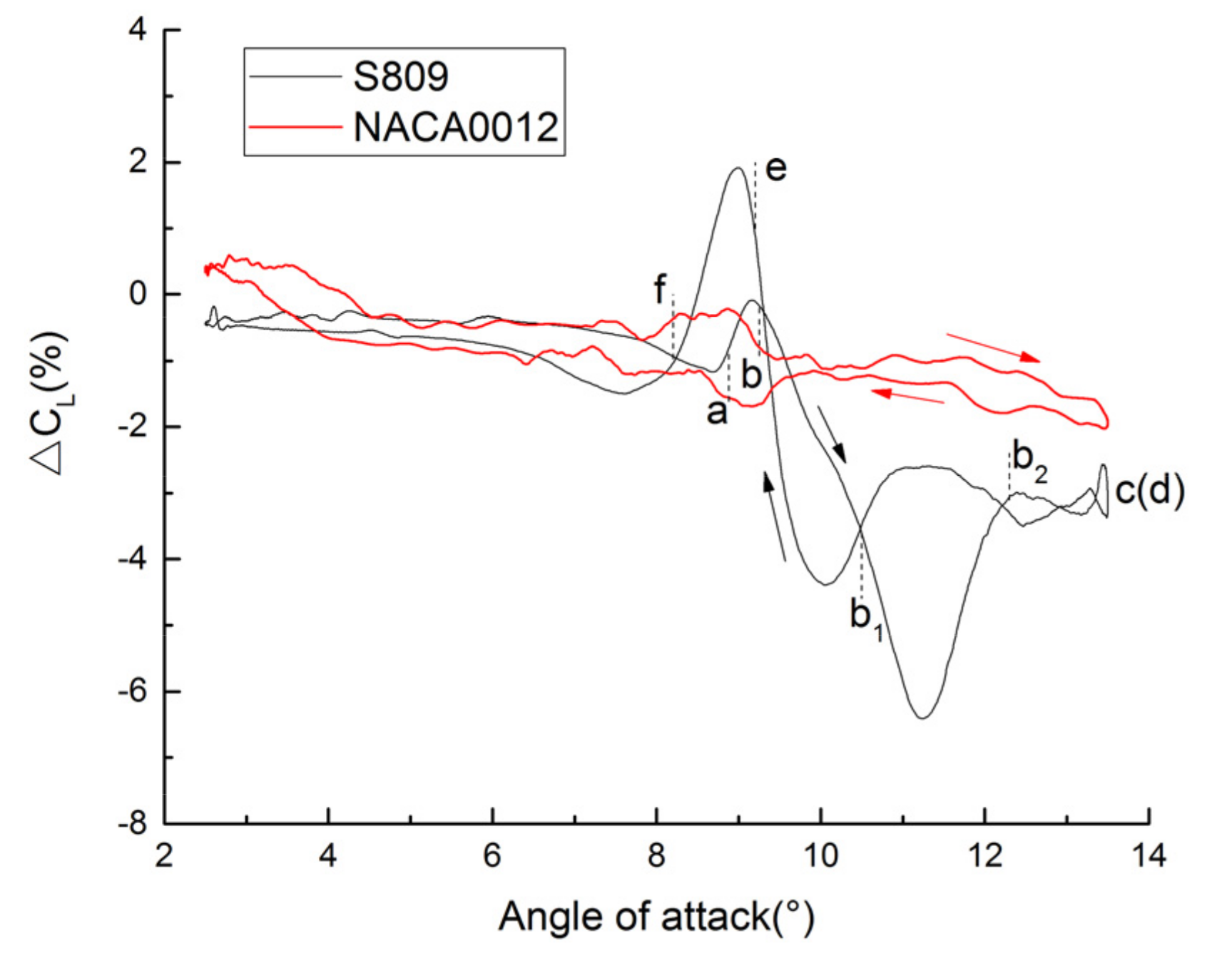
The reduced frequency has little effect on the value of the maximum increment of the lift coefficient caused by particles, but a larger one can enhance the hysteresis effect and change the angle of attack, at which the maximum increment is obtained, from the up stroke to the down stroke. The increment of the lift coefficient and its difference between two airfoils at a larger reduced frequency are smaller and larger during up and down strokes, respectively.

(2)

Compared to that of NACA0012 airfoil, the relative increments of S809 airfoil are obviously greater at three mean angles of attack, especially at 8°, which is the commonly used operating angle.

(3)

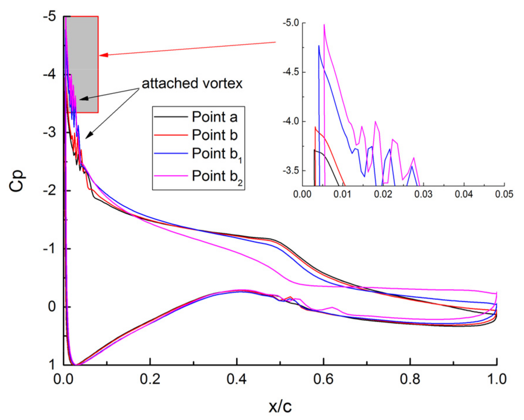
The angle of attack, at which the maximum lift coefficient is obtained, can be significantly changed by particles in two regions: one is under the effect of deep stall, the other is under the effect of light deep at a low reduced frequency.

References

1. Ham, N.D.; Young, M.I. Torsional Oscillation of Helicopter Blades Due to Stall. J. Aircr. 1966, 3, 218–224. [Google Scholar] [CrossRef]
2. Madden, P.A. Angle-of Attack Distribution of a High-Speed Helicopter Rotor. J. Am. Helicopter Soc. 1967, 12, 41–49. [Google Scholar] [CrossRef]
3. Carta, F.O. An Analysis of the Stall Flutter Instability of Helicopter Rotor Blades. J. Am. Helicopter Soc. 1967, 12, 1–18. [Google Scholar] [CrossRef]
4. Ham, N.D. Stall Flutter of Helicopter Rotor Blades: A Special Case of the Dynamic Stall Phenomenon. J. Am. Helicopter Soc. 1967, 12, 19–21. [Google Scholar] [CrossRef]
5. Ham, N.D.; Garelick, M.S. Dynamic Stall Considerations in Helicopter Rotors. J. Am. Helicopter Soc. 1968, 13, 49–55. [Google Scholar] [CrossRef]
6. McCroskey, W.; Carr, L.; McAlister, K. Dynamic Stall Experiments on Oscillating Airfoils. AIAA J. 1976, 14, 57–63. [Google Scholar] [CrossRef]
7. Mcalister, K.W.; Pucci, S.L.; Mccroskey, W.J.; Carr, L.W. An Experimental Study of Dynamic Stall on Advanced Airfoil Section. Volume 2: Pressure and Force Data. NASA Tech. Memo. 1982, 84245, 1–639. [Google Scholar]
8. Leishman, J.G.; Beddoes, T.S. A Semi-Empirical Model for Dynamic Stall. J. Am. Helicopter Soc. 1989, 34, 3–17. [Google Scholar]
9. Tuncer, I.H.; Wu, J.C.; Wang, C.M. Theoretical and Numerical Studies of Oscillating Airfoils. AIAA J. 1990, 28, 1615–1624. [Google Scholar] [CrossRef]
10. Raffel, M.; Kompenhans, J.; Wernert, P. Investigation of the Unsteady Flow Velocity Field above an Airfoil Pitching under Deep Dynamic Stall Conditions. Exp. Fluids 1995, 19, 103–111. [Google Scholar] [CrossRef]
11. Wernert, P.; Geiler, W.; Raffel, M.; Kompenhans, J. Experimental and Numerical Investigations of Dynamic Stall on a Pitching NACA 0012 Airfoil. AIAA J. 1996, 34, 982–989. [Google Scholar] [CrossRef]
12. Spentzos, A.; Barakos, G.; Badcock, K.; Richards, B.; Wernert, P.; Schreck, S.; Raffel, M. Investigation of Three-Dimensional Dynamic Stall Using Computational Fluid Dynamics. AIAA J. 2005, 43, 1023–1033. [Google Scholar] [CrossRef] [Green Version]
13. Liu, J.; Luo, K.; Sun, H.; Huang, Y.; Liu, Z.; Xiao, Z. Dynamic Response of Vortex Breakdown Flows to a Pitching Double-Delta Wing. Aerosp. Sci. Technol. 2018, 72, 564–577. [Google Scholar] [CrossRef]
14. Liu, J.; Chen, J.; Ren, H.; Zhang, Y.; He, X.; Xiao, Z. Correlations of Unsteady Vortex Burst Point and Dynamic Stability over a Pitching Double-delta Wing. Aerosp. Sci. Technol. 2020, 107, 106256. [Google Scholar] [CrossRef]
15. Yi, Y.; Hu, T.; Liu, P.; Qu, Q.; Eitelberg, G.; Akkermans, R.A. Dynamic Lift Characteristics of Nonslender Delta Wing in Large-amplitude-pitching. Aerosp. Sci. Technol. 2020, 105, 105937. [Google Scholar] [CrossRef]
16. Hu, T.; Zhao, Y.; Liu, P.; Qu, Q.; Guo, H.; Akkermans, R.A. Investigation on Lift Characteristics of a Double-delta Wing Pitching in Various Reduced Frequencies. Proc. Inst. Mech. Eng. Part. G J. Aerosp. Eng. 2021. [Google Scholar] [CrossRef]
17. Butterfield, C.P.; Simms, D.; Scott, G.; Hansen, A.C. Dynamic Stall on Wind Turbine Blades. In Proceedings of the American Wind Energy Association Conference: Windpower ‘91, Palm Springs, CA, USA, 1 December 1991; pp. 24–27. [Google Scholar]
18. Shipley, D.E.; Miller, M.S.; Robinson, M.C. Dynamic Stall Occurrence on a Horizontal Axis Wind Turbine Blade; Office of Scientific & Technical Information Technical Reports; National Renewable Energy Laboratory: Golden, CO, USA, 1995. [Google Scholar]
19. Ramsay, R.F.; Hoffman, M.J.; Gregorek, G.M. Effects of Grit Roughness and Pitch Oscillations on the S809 Airfoil; Office of Scientific & Technical Information Technical Reports; National Renewable Energy Laboratory: Golden, CO, USA, 1995. [Google Scholar]
20. Ekaterinaris, J.A.; Platzer, M.F. Computational Prediction of Airfoil Dynamic Stall. Prog. Aerosp. Sci. 1998, 33, 759–846. [Google Scholar] [CrossRef]
21. Larsen, J.W.; Nielsen, S.R.K.; Krenk, S. Dynamic Stall Model for Wind Turbine Airfoils. J. Fluids Struct. 2007, 23, 959–982. [Google Scholar] [CrossRef]
22. Sheng, W.; Galbraith, R.A.; Coton, F.N. A Modified Dynamic Stall Model for Low Mach Numbers. J. Sol. Energy Eng. 2007, 130, 653. [Google Scholar]
23. Pruski, B.J.; Bowersox, R. Leading-Edge Flow Structure of a Dynamically Pitching NACA 0012 Airfoil. Aiaa J. 2013, 51, 1042–1053. [Google Scholar] [CrossRef] [Green Version]
24. Liu, X.; Liang, S.; Li, G.; Godbole, A.; Lu, C. An Improved Dynamic Stall Model and Its Effect on Wind Turbine Fatigue Load Prediction. Renew. Energy 2020, 156, 117–130. [Google Scholar] [CrossRef]
25. Martinat, G.; Hoarau, Y.; Braza, M.; Vos, J.; Harran, G. Numerical Simulation of the Dynamic Stall of a NACA 0012 Airfoil Using DES and Advanced OES/URANS modelling. In Advances in Hybrid RANS-LES Modelling; Springer: Berlin/Heidelberg, Germany, 2008; Volume 97, pp. 271–278. [Google Scholar]
26. Martinat, G.; Braza, M.; Hoarau, Y.; Harran, G. Turbulence Modelling of the Flow Past a Pitching NACA0012 Airfoil at Formula Not Shown and Formula Not Shown Reynolds Numbers. J. Fluids Struct. 2008, 24, 1294–1303. [Google Scholar] [CrossRef] [Green Version]
27. Guntur, S.; Schreck, S.; Sorensen, N.N.; Schreck, S.; Bergami, L. Modeling Dynamic Stall on Wind Turbine Blades Under Rotationally Augmented Flow Fields; Technical Report; National Renewable Energy Laboratory: Golden, CO, USA, 2015. [Google Scholar]
28. Zhu, C.; Wang, T.; Zhong, W. Combined Effect of Rotational Augmentation and Dynamic Stall on a Horizontal Axis Wind Turbine. Energies 2019, 12, 1434. [Google Scholar] [CrossRef] [Green Version]
29. Li, G.; Zhang, W.; Jiang, Y.; Pengyu, Y. Experimental Investigation of Dynamic Stall Flow Control for Wind Turbine Airfoils Using a Plasma Actuator. Energy 2019, 185, 90–101. [Google Scholar]
30. Li, G.; Yi, S. Large Eddy Simulation of Dynamic Stall Flow Control for Wind Turbine Airfoil Using Plasma Actuator. Energy 2020, 212, 118753. [Google Scholar]
31. Zhu, C.; Chen, J.; Wu, J.; Wang, T. Dynamic Stall Control of the Wind Turbine Airfoil via Single-row and Double-row Passive Vortex Generators. Energy 2019, 189, 116272. [Google Scholar] [CrossRef]
32. Zhu, C.; Qiu, Y.; Wang, T. Dynamic Stall of the Wind Turbine Airfoil and Blade Undergoing Pitch Oscillations: A Comparative Study. Energy 2021, 222, 120004. [Google Scholar] [CrossRef]
33. He, T. Study the Dynamic Stall Characteristics of Wind Turbine Airfoil under Sand-wind Environment; Lanzhou University of Technology: Lanzhou, China, 2017. [Google Scholar]
34. Guo, T.; Jin, J.; Lu, Z.; Zhou, D.; Wang, T. Aerodynamic Sensitivity Analysis for a Wind Turbine Airfoil in an Air-Particle Two-Phase Flow. Appl. Sci. 2019, 9, 3909. [Google Scholar] [CrossRef] [Green Version]
35. Menter, F.R. Two-equation Eddy-viscosity Turbulence Models for Engineering Applications. AIAA J. 1994, 32, 1598–1605. [Google Scholar] [CrossRef] [Green Version]
36. Menter, F.R.; Langtry, R.B.; Likki, S.R.; Suzen, Y.B.; Huang, P.G.; Völker, S. A Correlation-Based Transition Model Using Local Variables-Part I: Model Formulation. J. Turbomach. 2006, 128, 413–422. [Google Scholar] [CrossRef]
37. Zhu, C.; Wang, T. Comparative Study of Dynamic Stall under Pitch Oscillation and Oscillating Freestream on Wind Turbine Airfoil and Blade. Appl. Sci. 2018, 8, 1242–1262. [Google Scholar] [CrossRef] [Green Version]
38. ANSYS Inc. FLUENT Theory Guide, Release 16.0; ANSYS Inc.: Canonsburg, PA, USA, 2015. [Google Scholar]
39. Morsi, S.A.; Alexander, A.J. An Investigation of Particle Trajectories in Two-Phase Flow Systems. J. Fluid Mech. 1972, 55, 193–208. [Google Scholar] [CrossRef]
40. Hand, M.M.; Simms, D.A.; Fingersh, L.J.; Jager, D.W.; Cotrell, J.R.; Schreck, S.; Larwood, S.M. Unsteady Aerodynamics Experiment Phase VI: Wind Tunnel Test Configurations and Available Data Campaigns; National Renewable Energy Laboratory: Golden, CO, USA, 2001. [Google Scholar]
41. Somers, D.M. Design and Experimental Results for the S809 Airfoil; National Renewable Energy Laboratory: Golden, CO, USA, 1997; pp. 1–97. [Google Scholar]
42. Luo, K.; Chen, S.; Cai, D.Y.; Fan, J.R.; Cen, K.F. Experimental Study of Flow Characteristics in the Near Field of Gas-Solid Two-Phase Circular Cylinder Wakes. Proc. Chin. Soc. Electr. Eng. 2006, 26, 116–120. [Google Scholar]
Figure 1. Computational field and mesh: (a) the blue and red semicircle edges are the velocity-inlet and pressure-outlet boundaries, respectively; (b) the green circle edge is the interface between the stationary domain and the rotating domain.
Applsci 11 10920 g001
Figure 2. Numerical and experimental data of time-varying aerodynamic coefficients: (a) lift coefficient loops; (b) moment coefficient loops.
Applsci 11 10920 g002
Figure 3. The streamwise velocity distributions of air in the wake of a circular cylinder at three Stokes numbers.
Applsci 11 10920 g003
Figure 4. Lift coefficient hysteresis loops of two airfoils in four cases in a clean air flow: (a) NACA0012 airfoil; (b) S809 airfoil.
Applsci 11 10920 g004
Figure 5. Pressure coefficients of four points for case 1.
Applsci 11 10920 g005
Figure 6. Lift coefficient hysteresis loops of two airfoils for Case 1: (a) NACA0012 airfoil; (b) S809 airfoil.
Applsci 11 10920 g006
Figure 7. Relative increment loops of two airfoils after loading particles with a concentration of 1%.
Applsci 11 10920 g007
Figure 8. Lift coefficient hysteresis loops of two airfoils for Case 2: (a) NACA0012 airfoil; (b) S809 airfoil.
Applsci 11 10920 g008
Figure 9. Relative increment loops of two airfoils after loading particles with a concentration of 1%.
Applsci 11 10920 g009
Figure 10. Lift coefficient hysteresis loops of two airfoils for Case 3: (a) NACA0012 airfoil; (b) S809 airfoil.
Applsci 11 10920 g010
Figure 11. Relative increment loops of two airfoils after loading particles with a concentration of 1%.
Applsci 11 10920 g011
Figure 12. Hysteresis loops of two airfoils for Case 4: (a) NACA0012 airfoil; (b) S809 airfoil.
Applsci 11 10920 g012
Figure 13. Hysteresis loops of two airfoils for Case 5: (a) NACA0012 airfoil; (b) S809 airfoil.
Applsci 11 10920 g013
Figure 14. Relative increment loops of two airfoils after loading particles with a concentration of 1%.
Applsci 11 10920 g014