Dilated Filters for Edge-Detection Algorithms

Abstract

Edges are a basic and fundamental feature in image processing that is used directly or indirectly in huge number of applications. Inspired by the expansion of image resolution and processing power, dilated-convolution techniques appeared. Dilated convolutions have impressive results in machine learning, so naturally we discuss the idea of dilating the standard filters from several edge-detection algorithms. In this work, we investigated the research hypothesis that use dilated filters, rather than the extended or classical ones, and obtained better edge map results. To demonstrate this hypothesis, we compared the results of the edge-detection algorithms using the proposed dilation filters with original filters or custom variants. Experimental results confirm our statement that the dilation of filters have a positive impact for edge-detection algorithms from simple to rather complex algorithms.

1. Introduction

An edge in an image is the most basic feature and has been intensively researched over time. A huge variety of mathematical methods have been used to identify points in which the image brightness changes sharply or has discontinuities. Edge detection is one low-level technique that is used for the goal of objects boundary detection. This is a fundamental tool in image processing, image analysis, machine vision and computer vision, particularly in the areas of feature detection and feature extraction.

The purpose of edge detection is to localize variations in the image and to identify the physical phenomena that produce them. Edge detection must be efficient and reliable to have the possibility of the completion of subsequent processing stages afterwards [1,2,3].

There are many approaches to basic feature detection depending on the pixel properties of the image. The methods have been defined from the gray scale levels to color slicing or from local features (such as lines or shapes) to global matching features (such as the shape of objects or meta object property). The standard local edge-detection filters are built for highlighting intensity change boundaries in the near neighborhood image regions. As previous authors have mentioned [4], the problem of edge finding has no universally accepted technique and this is a motivation for ongoing researching how to improve the edge detection methods.

The most successful edge-detection algorithms have considered local methods, where the closest neighborhood of a pixel is considered to be important for the pixel itself. Nowadays, images are containing more information than in the past (due to the sensors technologies) and we could say that the pixel itself is not similar only to its direct neighbors, but a bigger neighborhood could be important. From early morphological edge detection operators definition [5] the extension idea was well presented. From another perspective, the dilated convolution methods have been recently proven very beneficial in many highly cited computer-vision papers: for small objects detection [6], in dense prediction tasks [7,8], on prediction without losing resolution [9], for feature classifications in time series [8] or beneficial for context aggregation [10].

Merging those ideas we propose not just to increase the filter size but to simply dilate standard edge-detection filters in order to characterize the pixel itself through non-direct neighbor properties. We define the dilation operation for filters that consists of simply adding gapes in the well-known classical filters. This method of dilation is neither in the mathematical morphological sense [5], nor the geometric extension of the kernels discussed in the literature [11].

In our previous work we evaluated the dilation effect on classical first-order edge-detection algorithms and the classical Canny algorithm followed, naturally, with an analysis on which approach is better: to expand from lower level or to dilate, see [11,12]. The result of the evaluation revealed that dilating the filter produces better results than expanding them. These initial set of positive results encouraged us to further investigate this topic. In Figure 1 we can observe the effect on a edge-detection algorithm when applying the dilated kernel. To better show the benefits we used green edge pixels to highlight discovered by dilating and red for the edge pixels that are lost by dilatation techniques.

In order to obtain the edge maps presented in Figure 1, we used the Canny algorithm [13] with the exact parameters (Gaussian sigma value, low threshold and high threshold) and changed just the filter with a dilated version. As we can observe in the images, each level of dilation can bring with it extra edge points. This aspect can be a benefit for the overall results and in this manuscript we desire to explore this aspect. In Figure 2 we present results of Canny algorithm with different thresholds. From left to right we use a higher combination of thresholds and the rows represent the filters, from classic to dilated. As a brief interpretation of the results one can say that dilation is sensitive to artifacts at lower threshold. On the other hand, in the last column, for a higher threshold, dilated filters discover new edge points. These outcome that we see in Figure 1 and Figure 2 encouraged us to investigate the benefits of dilating on different algorithms in the future.

In this paper we desire to extend our work to other edge-detection algorithms that have as a defining step the use of edge detection kernels. The classical edge detection methods Sobel [14], Prewitt [15] and Scharr [16], together with more complex boundary detection algorithms such as Canny [13], Marr–Hildreth [17] or Shen–Castan [18] are considered for testing with our proposed dilation technique. With this extended research work we wish to prove the research hypothesis that dilatation of kernels can bring forward better edge maps.

The main contributions of this paper are summarized as follows:

• Extend our previous analysis on first-order derivative orthogonal gradients based algorithms and Canny algorithm, that was performed in Bogdan et al. [11].
• Analyze and evaluate the effect of dilated filters upon first-order derivative compass gradient based algorithms, Frei–Chen algorithm [19,20] and Edge Drawing algorithm [21].
• Analyze and evaluate the effect of dilated filters upon second-order derivative based algorithms such as: Laplacian [22], Laplacian of Gaussian [23], Marr–Hildreth or Shen–Castan.
• Analyze and evaluate if the effect of dilated is maintained when using different kernels for the mentioned algorithms.
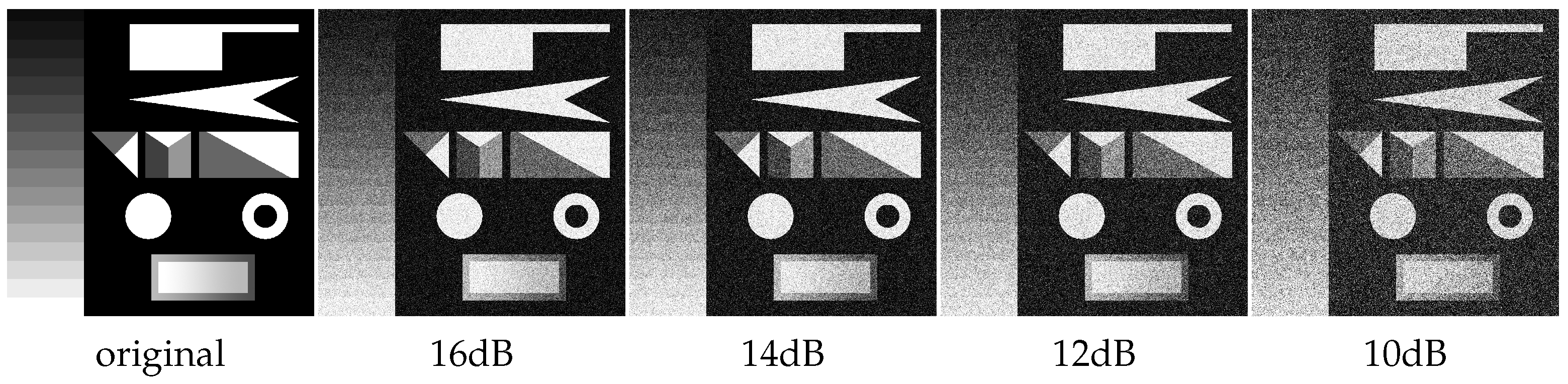
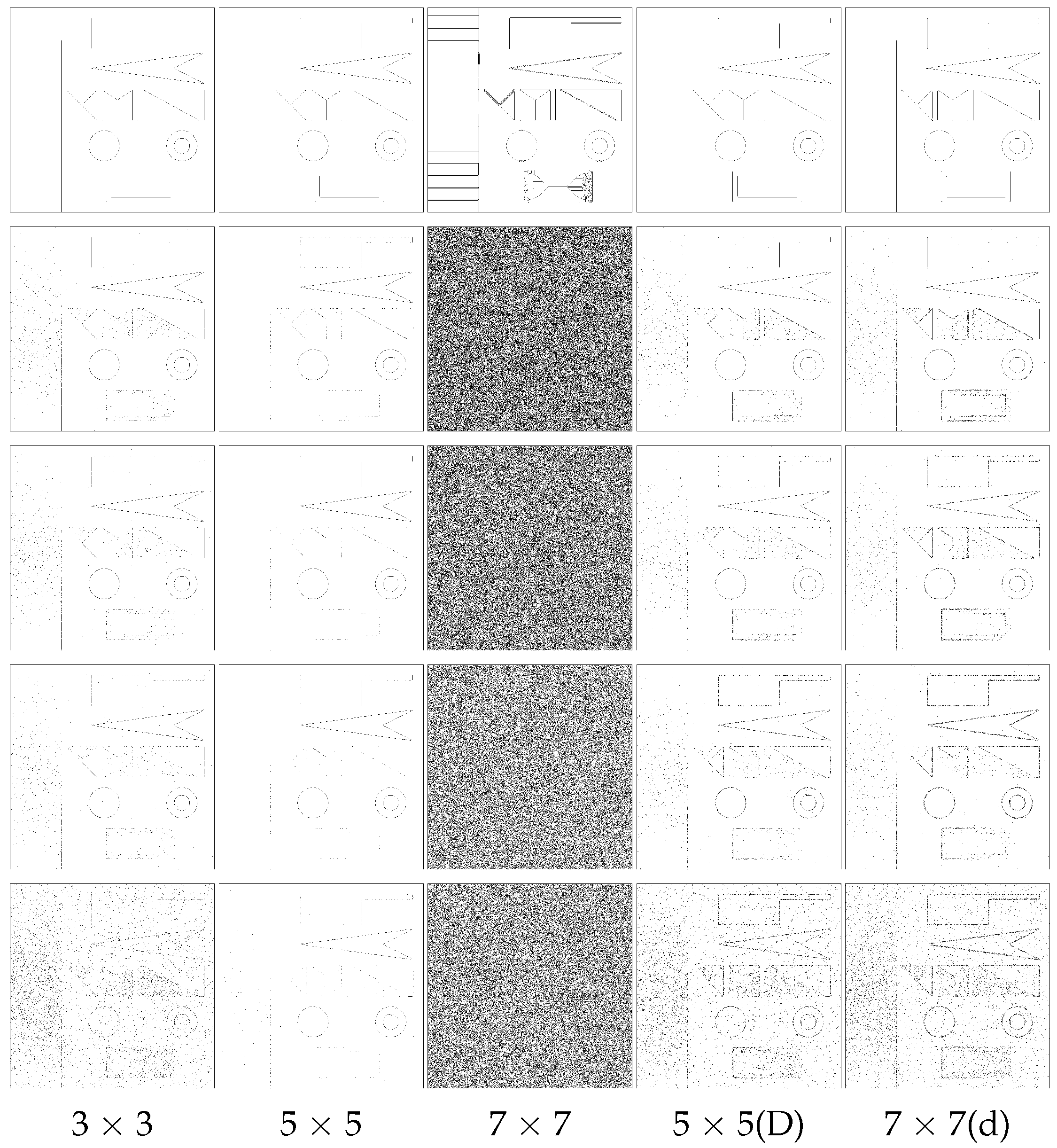
• Analyze and evaluate the effect of noise level of an input image upon the dilated filters.
• Prove the research hypothesis that dilated filters in general bring forward better results than classical or extended versions of them.

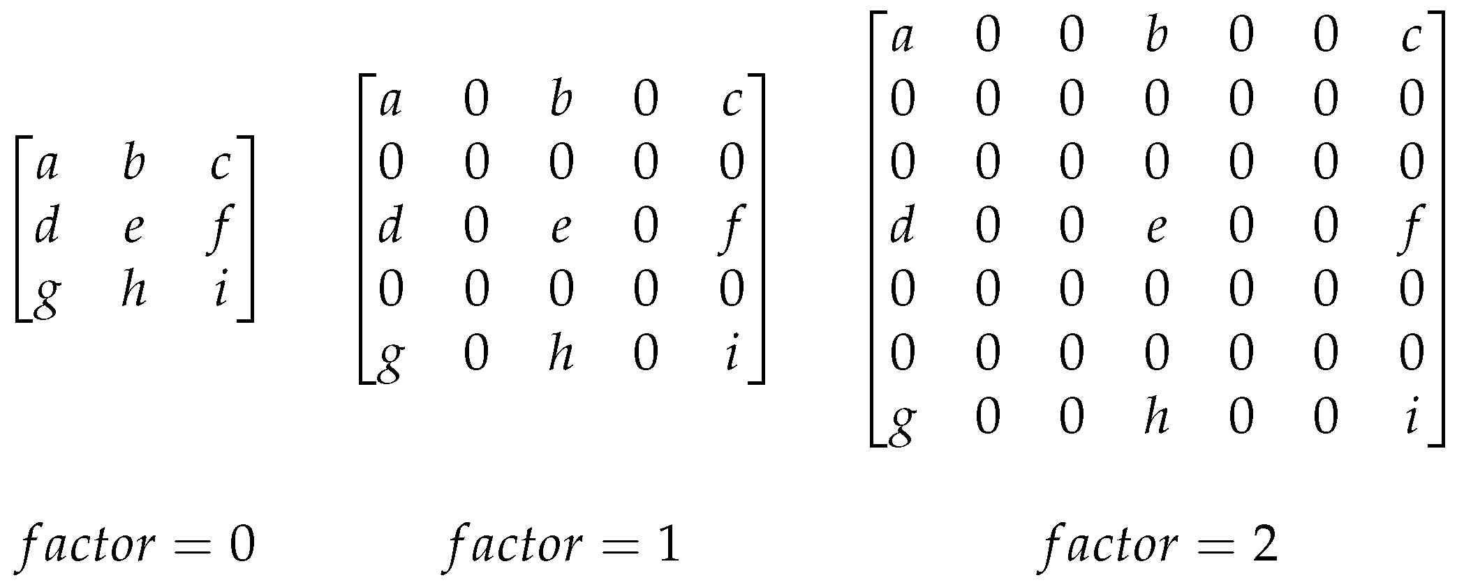
In order to complete our evaluation of the dilation benefits over an edge-detection filter, we will not limit our analysis to the first-order derivative gradient-based edge-detection filters but consider the second-order filter too. Details regarding the new approached algorithms and steps we used in order to obtain the edge map format are presented in Section 3. Section 4 highlights the new results of our hypothesis regarding the dilated filters. For completing the comparison we used two different datasets and evaluation measures, one based on natural images and one based on synthetic images, that are presented in Section 3.11.

2. Dilated Filters

In order to benefit from a higher neighborhood of a pixels to obtain a pixel edge we define dilated filter as in Definition 1. When we dilate the kernels, we are considering the newly added positions as gaps and we ignore them by setting zeros [11]. We can admit that dilating the kernels can cause a noise sensitivity reduction in the kernel; however, from our experiments, from this and previous work, it seems that it is an acceptable loss considering the benefits.

Definition 1.

A dilated filter is obtained by expanding the original filter by a dilation factor [11].

By dilating the kernels we increase the distance between important pixels. We consider that this new distance will positively influence the result of the convolution. The bigger region of interest resulted can translate into stronger intensity changes in the image. In order to highlight our definition on a filter, we use a generic kernel and represent the dilation in Figure 3.

Dilating the filters, rather than extending them, helps in finding more edge pixels than the standard or extended variants of the filters. Another benefit worth mentioning of dilating is the fact that the number of operations does not increase with the dilating factor resulting in the same time cost for the edge detection [11].

Another considered approach was presented in [12], where we compare and analyze the dilation of filters defined in [11] with the reconstruction from a lower scale pyramid level. Feature extraction in lower pyramid scale level is a common practice in the domain because of the benefits of lower computation resources which are needed.

The resulting edge map from a dilated 3 × 3 filter is equivalent to an edge map calculated in a lower scale pyramid level and expanded back to original size. Dilating a factor of one is similar with applying the same filter in the immediately lower scale pyramid level. Dilating with a factor of two is similar with applying the filter in two scales lower in pyramid level and so on. This hypothesis stands because in both cases the region we take into consideration to find edges is no longer a 3 × 3 matrix but a 5 × 5 matrix.

We have examined the equivalence between lower level processing and dilating in our previous work [12]. As expected, we obtain similar results when dilating to when processing in the lower levels. Dilating provides benefits regarding the neighborhood we consider and computation time; however, extracting features in lower levels has benefits of its own.

3. Methodology

In this section, we present all the edge-detection algorithms that are considered in our analysis. The presentation order of the algorithms is in order of their implementation in our experiments.

For our evaluation, we chose to use the classical version of the algorithm and variants in which the users are responsible for choosing the parameter configuration for each algorithm. Even if these approaches are more costly than choosing an automated threshold scheme [24,25,26,27,28,29,30], they provide us the possibility to better highlight the effect of the kernel dilatation. By using the original version of each algorithm we avoid bringing in the evaluation suppositions or assumptions that are made by the parameter choosing scheme.

In order to benchmark our results, all the edge maps need to have the values of the pixels between 0 and 255 and thickness of 1 pixel. To achieve this, we use a global thresholding algorithm followed by a thinning algorithm where this is necessary. For thinning the resulting edge maps, we use the Guo–Hall algorithm [31].

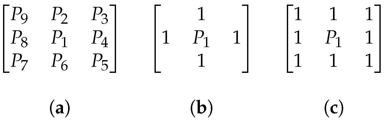
3.1. Guo–Hall Algorithm

The Guo–Hall algorithm [31] is one of the most efficient thinning algorithms and is based on a subiteration approach of alternatively deleting north and east and then south and west boundary pixels. If we have one group of 8-connected 1s around a position P, see Figure 4, the deletion of P will not break the connectivity of the elements in a 3 × 3 window. This approach on thinning will preserve the connectivity properties of an image.

For an input binary image, let the object to be thinned be represented by a set S, and the background and holes in the image be represented by a complement set $\overline{S}$ [31].

Thinned lines should be a curve or a union of curves, which are referred to as medial curves. A set of pixels G, is curve-like if most of the pixels of G have exactly two 8-neighbors in G, a few pixels in G are end-points (with one 8-neighbors in G) or branch points (more than two 8-neighbors in G) [31].

Let us define the following: $C\left(P_1\right)$ is defined as the number of distinct 8-connected components of 1s in the 8-neighborhood; ∧ as the AND operator; ∨ as the OR operator;  $\overline{}$  as a logical complement. A variable $N\left(P_1\right)$, defined in Equation (1), helps with the detection of end-points as well as achieving thinner results. The $N_1\left(P_1\right)$ and $N_2\left(P_1\right)$ are defined in Equations (2) and (3). Each break the ordered set of $P_1$’s neighboring pixels into four pairs of adjoining pixels and count the number of pairs that contain one or two 1 s [31].

$$\begin{array}{c}\hfill N\left(P_1\right)=min[N_1\left(P_1\right),N_2\left(P_1\right)]\end{array}$$

(1)

$$\begin{array}{c}\hfill N_1\left(P_1\right)=(P_9\vee P_2)+(P_3\vee P_4)+(P_5\vee P_6)+(P_7\vee P_8)\end{array}$$

(2)

$$\begin{array}{c}\hfill N_2\left(P_1\right)=(P_2\vee P_3)+(P_4\vee P_5)+(P_6\vee P_7)+(P_8\vee P_9)\end{array}$$

(3)

The algorithm that is applied for each pixel $p(i,j)$ is defined in Algorithm 1. The conditions in the algorithm are necessary for preservation of local connectivity when $P_1$ is deleted and avoids deletion of pixels in the middle of medial curves.

Algorithm 1 Guo–Hall Algorithm.

1: while points are deleted do 2:     for all pixels p(i, j) do 3:         if odd iterations then 4:            if $C\left(P_1\right)=1$$AND$$2\le N\left(P_1\right)\le 3$$AND$$(P_2\vee P_3\vee \overline{P_5})\vee P_4=0$ then 5:                Delete pixel p(i, j) 6:            end if 7:         else 8:            if $C\left(P_1\right)=1$$AND$$2\le N\left(P_1\right)\le 3$$AND$$(P_6\vee P_7\vee \overline{P_9})\wedge P_8=0$ then 9:                Delete pixel p(i, j) 10:            end if 11:         end if 12:     end for 13: end while

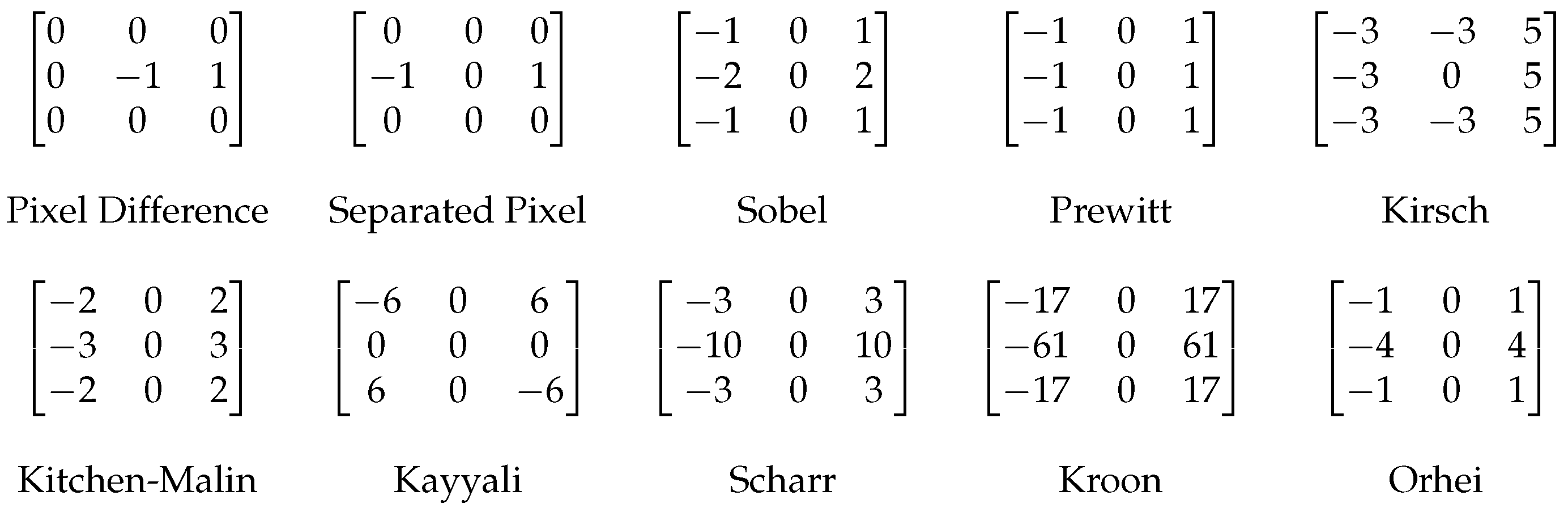
3.2. First-Order Derivative Orthogonal Gradient Operators

First-order derivative orthogonal gradient operators are the most basic operators and have been extensively researched over the decades. We consider in our analysis the following edge-detected operators and their extensions: pixel difference operator [32], separated pixel difference operator [32], Sobel operator and the extension to a 5 × 5 or 7 × 7 kernel [33,34,35,36,37], Prewitt operator and the extension to a 5 × 5 or 7 × 7 kernel [34,36], Kirsch operator [38] and the 5 × 5 kernel expansion [33], Kitchen and Malin operator [39], Kayalli operator, Scharr operator and the extensions to 5 × 5 kernel [36,40], Kroon operator [41] and Orhei operator [42].

All the kernel masks for the operators are presented in Figure A1, Figure A3 and Figure A6 from Appendix A. All those operators are orthogonal discrete filters so we represent only one of the kernels. To obtain the other kernels we just need to rotate it by a fraction of $\frac{\pi }{2}$.

The gradient is a measure of change in a function, and an image can be considered to be an array of samples of some continuous function of image intensity, typically the two-dimensional equivalent of the first derivative. The magnitude is calculated using Equation (4), where $f(x,y)$ is the image and $G_x$, $G_y$ are the gradient elements on x and y directions. The direction of the gradient is calculated using Equation (5) [23].

$$\begin{array}{c}\hfill G\left[f(x,y)\right]=\sqrt{G_x^2+G_y^2}\approx |G_x|+|G_y|\end{array}$$

(4)

$$\begin{array}{c}\hfill \theta ={tan}^{-1}\left[\frac{G_y}{G_x}\right]\end{array}$$

(5)

The result of this algorithm is an edge map formed by edges that are not topically 1 pixel width, this aspect can deform the result of our evaluation. So for a better evaluation, we choose to thin the resulting edges beforehand using the Guo–Hall algorithm [31]. We add two steps to this algorithm that are commonly used, see [43]: smoothing and thresholding. Smoothing of images is a common practice for enhancing the results as thresholding will eliminate “weak” edges that are found. We present the flowchart for these edge detections in Algorithm 2.

Algorithm 2 First-Order Derivative Operators steps.

Input: RGB image      Output: Binary edge map      Parameters: Sigma value (S), Gradient Threshold (TG) 1: for edge operator do 2:     Convert image to gray-scale image 3:     Apply Gaussian filter smoothing 4:     Apply convolution with kernel      ▹kernel rotated with $\pi /2$, found in Figure A1 (for Gradient magnitude)      ▹kernel rotated by a fraction of $\pi$, as in Figure A2 (for Compass magnitude)      ▹kernel found in Figure A7 (for Frei–Chen) 5:     Calculate gradient magnitude using     ▹Equation (4) (for Gradient magnitude)     ▹Equation (6) (for Compass magnitude)     ▹Equation (7) (for Frei–Chen) 6:     Apply global threshold algorithm 7:     Apply Guo–Hall thinning algorithm [31] to remove the excess edge points 8: end for

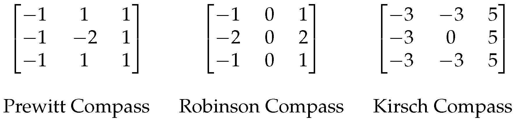
3.3. First-Order Derivative Compass Gradient Operators

Compass gradient operators are commonly used in the edge detection and usually detect the influence of the neighbor pixels in a compass rotating directional components. They are commonly used as an alternative for the orthogonal gradient operators.

The gradient magnitude is calculated using Equation (6), where: k is the number of kernels and L is the kernel size minus 1, divided by 2; z is the rotation index; g represents the kernel and f the image. The resulting value of intensity is normalized or thresholded to eliminate low confident edges. The local edge orientation is estimated with the orientation of the kernel that yields the maximum response, as in [44,45].

$$\begin{array}{c}\hfill G\left[f(x,y)\right]=\underset{z=k}{max}\sum _{i=-L}^L\sum _{j=-L}^L{g}_{ij}^{\left(z\right)}\ast f(x+i,y+j)\end{array}$$

(6)

The operators are also orthogonal discrete filters so we represent and use only $G_x$ kernel. To obtain the other kernels for this template gradient we need to rotate it by a fraction of $\pi$, different from the previous ones.

For our analysis we found in the literature the following: Prewitt Compass operator [15], Robinson Compass operator [15,46] and Kirsch operator. All kernel mask details can be found in Figure A2 from Appendix A.

Similar to orthogonal gradient operators, because the resulting edge map is not 1 pixel width, neither with the same magnitude, we threshold and thin the results before the evaluation. Similar to other algorithms to obtain the better results we apply a smoothing process using the Gaussian filter before performing the edge detection. Details are presented in Algorithm 2.

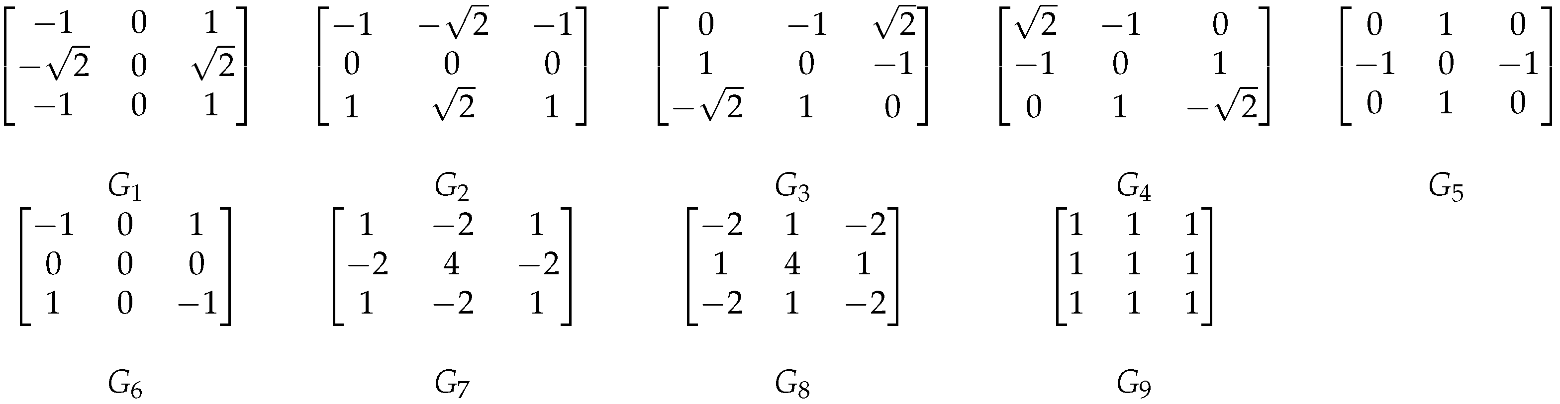
3.4. Frei–Chen Operator

The Frei–Chen operator works on a 3 × 3 footprint but applies a total of nine convolution masks to the image. The masks one through nine, defined a 3 × 3 window span of the edge, line and average subspaces. All the kernel masks for the operators are presented in Figure A7 from Appendix A. Kernels $G_1$ and $G_2$ are isotropic average gradient basis vectors and kernels $G_3$ and $G_4$ are the ripple vectors, all of them contributing to the edge detection subspace. Kernels $G_5$ and $G_6$ are the line basis vectors, respective kernels $G_7$ and $G_8$ are the discrete Laplacian vectors and are used for the line subspace detection. From [19], Kernel $G_9$ is the average mask.

To use the Frei–Chen operator for edge detection we apply Equation (7) for the first 4 masks. For line detection Equation (8) be used with the next 4 masks.

$$\begin{array}{c}\hfill G{\left[f(x,y)\right]}_{edge}=\sqrt{\frac{{\displaystyle \sum _{k=1}^4}{\left(G_k\right)}^2}{{\displaystyle \sum _{k=1}^9}{\left(G_k\right)}^2}}\end{array}$$

(7)

$$\begin{array}{c}\hfill G{\left[f(x,y)\right]}_{line}=\sqrt{\frac{{\displaystyle \sum _{k=4}^8}{\left(G_k\right)}^2}{{\displaystyle \sum _{k=1}^9}{\left(G_k\right)}^2}}\end{array}$$

(8)

In some way, the Frei–Chen operator is a first-order derivative compass gradient operator, and we treat it as such. The evaluation steps are: the image is smoothed using a Gaussian filter, the resulting edge map is thresholded and in the last step the edge map is thinned. In our evaluation, we only considered the results for edge detection; to this end, we used Equation (7), see Algorithm 2.

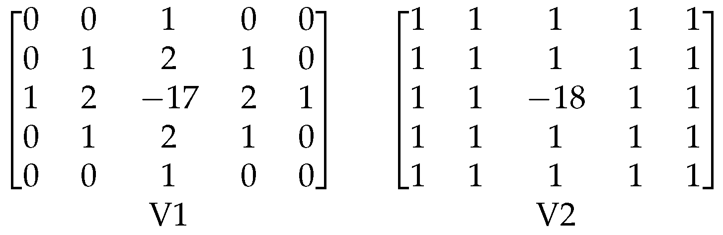
3.5. Laplacian Edge Operator

The Laplacian is a 2D isotropic measure of the second spatial derivative of an image. The Laplacian of an image highlights regions of rapid intensity change and is therefore often used for edge detection. Another difference between Laplacian and other operators is that Laplacian does not take out edges in any particular direction. The formula for the Laplacian is the second-order derivative by each component of a 2D function as is presented in Equation (9).

$$\begin{array}{c}\hfill {\nabla }^{2}f(x,y)=\frac{{\partial }^{2}f(x,y)}{\partial x^2}+\frac{{\partial }^{2}f(x,y)}{\partial y^2}\end{array}$$

(9)

From the literature [22,23,45,47] we can find different estimations of isotropic kernels for the Laplacian operator that we present in Figure A4 and Figure A5 in Appendix A. For our work, we consider all of them so we can highlight changes that appear on the edge map when choosing different approximations of the Laplace function.

We apply Equation (9) to obtain the raw edge map; however, to be able to evaluate, we need to transform the edge result from natural range of ($-256$, 255) to (0, 255). The obtained scaled edge map, which now has only positive values, is thinned using the Guo–Hall algorithm for the final result. We can accept that this is not the normal usage of the Laplace operator but we wanted to evaluate it separately from Laplace of Gaussian or Marr–Hildreth operators. The details are presented in Algorithm 3.

Algorithm 3 Laplace and LoG Operator steps.

Input: RGB image      Output: Binary edge map      Parameters: [Sigma value (S) − only LoG], Gradient Threshold (TG), 1: for edge operator do 2:     Convert image to gray-scale image 3:     Apply edge detection operator using     ▹Equation (9) (for Laplace Operator)     ▹Equation (10) (for LoG) 4:     Scale the edge pixels from ($-256$, 255) to (0, 255) range 5:     Apply global threshold algorithm 6:     Apply Guo–Hall thinning algorithm [31] to remove the excess edge points 7: end for

3.6. Laplacian of Gaussian—LoG—Or Mexican Hat Operator

The Laplacian of Gaussian (LoG) approach is that the image is convoluted with a Gaussian filter to reduce the noise followed by a Laplacian convolution to expose the edges. The LoG function with the three-dimensional plot looks similar to a Mexican hat, hence the name of the operator [23,48]. We can use two mathematical variants for obtaining LoG, (see Equation (10)): convolve the image with a Gaussian smoothing filter and afterwards compute with the Laplacian operator, or convolve the image with the linear filter that is the Laplacian of the Gaussian filter (Equation (11)).

$$\begin{array}{c}\hfill LoG(x,y)={\nabla }^2\left[\left(g\right(x,y)🟉f(x,y\left)\right)\right]={\nabla }^2\left[g(x,y)\right]🟉f(x,y)\end{array}$$

(10)

$$\begin{array}{c}\hfill {\nabla }^{2}g(x,y)=-\frac{1}{\pi {\sigma }^4}\left[1-\frac{x^2+y^2}{2{\sigma }^2}\right]e^{-\frac{x^2+y^2}{2{\sigma }^2}}\end{array}$$

(11)

Similar to the Laplace operator, we need to transform the resulted edge map from range of ($-250$, $+250$) to a (0, 250) so the determined edge map is scaled followed by thresholding and thinning. The details are presented in Algorithm 3.

3.7. Marr–Hildreth Algorithm

Another method of detecting edges in digital images is the Marr–Hildreth algorithm, which is used in continuous curves that feature strong and rapid variations in image brightness.

The Marr–Hildreth edge detection method is simple and operates by convolving the image with the Laplacian of the Gaussian function, or, as a fast approximation by difference of Gaussian. Zero crossings are detected in the filtered result to obtain the edges. A zero crossing at pixel level implies that the signs of at least two opposite neighboring pixels are different [17,49].

For our implementation of the zero crossing algorithm, we chose to implement a threshold that permits us to discriminate better relevant zero crossing according to the difference in intensity [49,50]. This variant of zero crossing produces better results than the classical version that threshold the results at zero regardless of intensity change. All the steps used for simulations are presented in Algorithm 4.

Algorithm 4 Marr–Hildreth Operator steps.

Input: RGB image   Output: Binary edge map   Parameters: Sigma value (S), Gradient Threshold (TG), 1: for edge operator do 2:       Convert image to gray-scale image 3:       Apply edge detection operator using Equation (10) 4:       Apply Zero Crossing [49] algorithm 5:       Apply Guo–Hall thinning algorithm [31] to remove the excess edge points 6: end for

3.8. Canny Algorithm

The Canny edge-detection algorithm is a classical and robust method for edge detection in gray-scale images. The edge-detection algorithm is widely used due to its short operation time and relatively simple calculation process.

The traditional Canny algorithm has the following steps: (1) smooth the image with a Gaussian function, (2) apply the first-order operator, (3) non-maximum suppression of the magnitude of the gradient and (4) double threshold is used for edge connections. The classic Canny algorithm is presented in Algorithm 5.

Non-maximum suppression is an important step for the Canny algorithm. The purpose of it is to find the local maximum value of the pixels, and set the gray value corresponding to the non-maximum point to zero, so that a large part of non-edge points can be eliminated. It is a technique through which the edges are made thinner by checking, for each edge pixel, if the adjacent pixels which fall between the gradient angle have a smaller value. If not, the edge pixel is suppressed [13].

After the non-maximum suppression phase using the two thresholds, we double threshold and edge link by hysteresis the edge points. If an edge pixel’s gradient value is higher than the high threshold it is set as a strong edge pixel. Similarly, if an edge pixel’s gradient value is smaller than the high threshold value but larger than the low threshold value, it is marked as a weak edge pixel. If an edge pixel’s gradient value is smaller than the low threshold value, it will be suppressed. At the end, the remaining “weak” and “strong” pixels are connected as long as there is one strong edge pixel that is involved in the blob.

Algorithm 5 Canny Operator steps.

Input: RGB image   Output: Binary edge map   Parameters: Sigma value (S), Low Threshold (TL), High Threshold (TH), 1: for edge operator do 2:       Convert image to gray-scale image 3:       Apply Gaussian filter smoothing 4:       Apply convolution with kernels on the x and y axes 5:       Calculate gradient magnitude with their kernels on the x and y axes 6:       Apply non-maximum suppression, as in [13] 7:       Apply edge tracking by hysteresis using double threshold 8: end for

3.9. Shen–Castan Algorithm

The unique feature of the Shen–Castan algorithm is that it uses the infinite symmetric exponential filter ($\mathrm{ISEF}$) [18], which offers better noise reduction. The detection steps used by Shen–Castan and Canny are similar, but the Shen–Castan $\mathrm{ISEF}$ filter provides better signal-to-noise ratios and better localization. The implementation of Canny’s algorithm approximates his optimal filter by the derivative of a Gaussian, whereas Shen–Castan uses the optimal filter directly [51].

ISEF is described as a real continuous function for one dimension by Equation (12) and for two dimensions by Equation (13), where p is the thinning factor and a is the normalization coefficient; more details can be seen in [52]. To speed up the convolution, we used the discrete version of ISEF, the recursive filter, Equation (14), where b is the thinning factor and its values lie in between 0 and 1.

$$\begin{array}{c}\hfill f\left(x\right)=\frac{p}{2}{e}^{-p\left|x\right|}\end{array}$$

(12)

$$\begin{array}{c}\hfill f(x,y)=a·e^{-p\left(\right|x|+|y\left|\right)}\end{array}$$

(13)

$$\begin{array}{c}\hfill f(x,y)=\frac{(1-b)·b^{\left(\right|x|+|y\left|\right)}}{1+b}\end{array}$$

(14)

Shen–Castan edge detector has a unique step that overcomes noise in the input image by using the ISEF, see [53]. The algorithm has the following steps: (1) smooth the image with the ISEF filter, (2) convolve the smoothed image with a Laplace binary operator, (3) threshold the edge strong edge pixels using zero crossing, (4) link the edge points by hysteresis and (5) thin the results at the end. Details regarding the steps we use for obtaining the edge map are presented in Algorithm 6.

The approximation of the Laplacian is computed by subtracting the original image from the smoothed one. The result is a band-limited Laplacian image. Next, a binary Laplacian image is generated by setting all the positive valued pixels to 1 and all others to 0, as in [53].

For our analysis we do not use the Laplace binary operator, which is considered to be optimal as run time for this algorithm but instead use the versions of Laplace isotropic kernels presented in Section 3.5.

Algorithm 6 Shen–Castan Operator steps.

Input: RGB image   Output: Binary edge map   Parameters: Smoothing Factor of ISEF (SF), Threshold of Laplace (TG), Zero crossing window (W), Threshold for zero crossing (R), Thinning Factor (TN) 1: for edge operator do 2:       Convert image to gray-scale image 3:       Apply recursive ISEF filter smoothing 4:       Apply Laplace Operator 5:       Apply Zero Crossing replacing the pixel values by 1 for positive and 0 for negative 6:       Apply non-maximum suppression using adaptive gradient method with fixed width W 7:       Apply edge tracking by hysteresis using double threshold 8: end for

3.10. Edge-Drawing Algorithm

Edge drawing (ED) is an edge-detection algorithm that works by computing a set of anchor points, which are most likely to be edge elements, and linking them with a predefined set of rules, which we call smart routing [21].

The ED algorithm can be summarized in the following steps: smooth the image with a Gaussian filter [54], calculate the gradient magnitude and orientation using Sobel filter, extract the anchor points and connect the anchor points using the smart routing concept. The steps of the ED algorithm are presented in Algorithm 7.

The mechanism of connecting anchors is considered the most crucial step of ED. Connecting consecutive anchors is achieved by passing from one anchor to the next following the cordillera peak of the gradient map mountain. This process, as in [21], is guided by the gradient magnitude and edge direction maps computed. If a horizontal edge passes through the anchor, we start the connecting process by proceeding to the left and to the right. If a vertical edge passes through the anchor, we start the connection process by proceeding up and down. The process stops if we move out of the edge area or we encounter a previously detected edge.

Algorithm 7 Edge Drawing Operator steps.

Input: RGB image   Output: Binary edge map   Parameters: Gaussian Kernel (GK), Threshold of Laplace (TG), Anchor Threshold (TA), Scan Interval (SI) 1: for edge operator do 2:       Convert image to gray-scale image 3:       Apply Gaussian filter smoothing 4:       Apply convolution with kernel rotated with $\pi /2$, found in Figure A1 5:       Calculate direction map if $|G_x|\ge |G_y|$ vertical edge otherwise horizontal edge 6:       Apply a global threshold scheme by $TG$ value 7:       Extract anchors using $TA$ and $SI$ 8:       Smart routing 9: end for

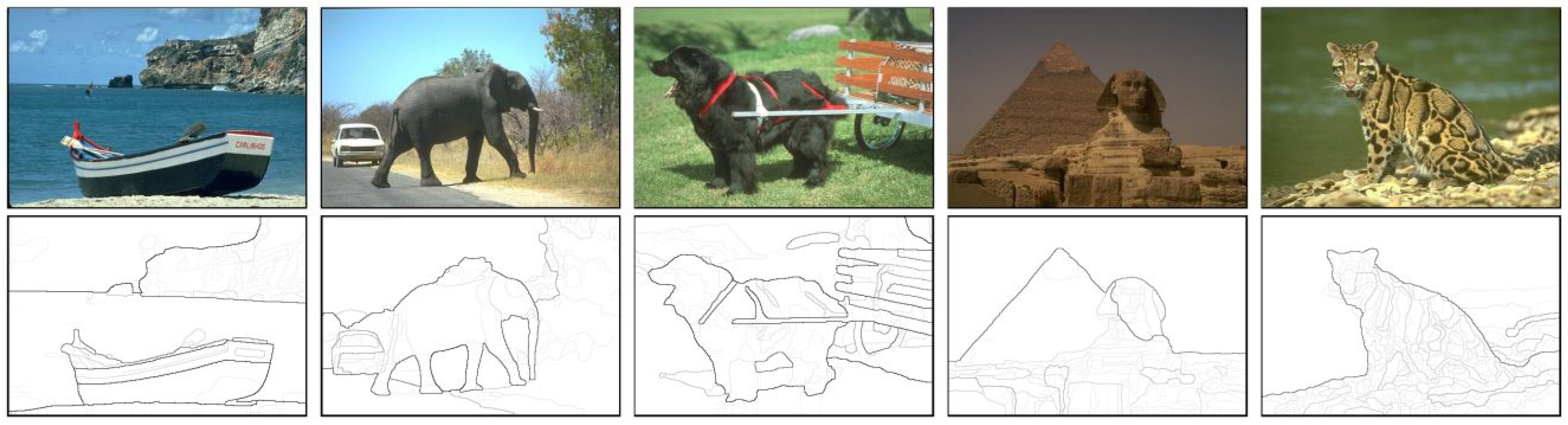
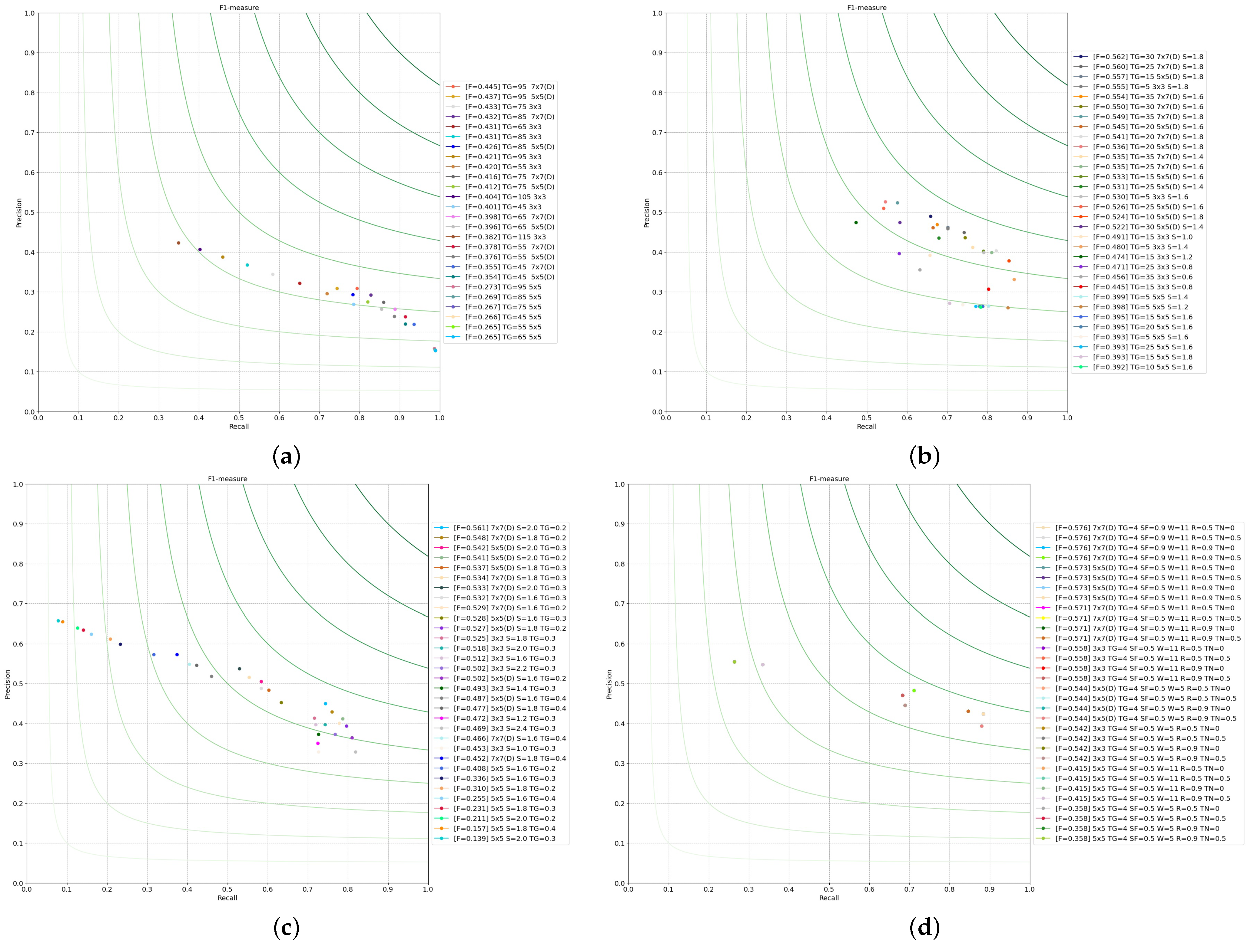
3.11. Benchmarking the Edge Operators

Edge-detection evaluation methods are an important aspect and multiple solutions are presented in the literature, but it still is a challenging and not totally solved problem. Edge-detection evaluation methods can be categorized in several ways. First, they can be classified as subjective or objective methods. The subjective method uses human observation to decide the edge detection evaluation. In objective methods, quantitative measures are defined based solely on images and the edge-detection results. Secondly, edge-detection evaluation methods can be categorized based on test images: synthetic-image-based methods and real-image-based methods [55,56,57].

In edge detection evaluation, the measurement process can be classified as: unsupervised or supervised evaluation criteria. The first method concerns only the input data image and generates a score of coherence that qualifies the algorithm result. The second computes a similarity/dissimilarity measure between the resulted image and a ground truth obtained from synthetic data or an expert judgment [58].

Multiple evaluation schemes are found in the literature for measuring supervised evaluation criteria, as in [3,58,59,60]. For the evaluation of edge detection, the confusion matrix remains a cornerstone in boundary detection evaluation methods. If we consider the ground truth image as $I_{gt}$ and the predicted image as $I_p$ we have the following possible set of points:

• True positive points (TPs), common points of $I_{gt}$ and $I_p$.
• False positive points (FPs), false detected edges of $I_p$.
• False negative points (FNs), missing edge points of $I_p$.
• True negative points (TNs), common non-edge points.

To evaluate our proposed algorithms, we used two different supervised evaluation criteria on two different datasets: one synthetic and one constructed on expert judgment. In order to select the correct dataset, we analyzed multiple datasets [12,61,62,63,64,65,66,67,68]. For the expert judgment, we used the Berkeley Segmentation Data Set and Benchmarks 500 ($BSDS500$) in correlation with the pixel corresponding metric ($PCM$) [69]. Regarding the synthetic dataset, we used the dataset from [12] in correlation with the symmetric figure of merit [58] ($SFoM$) metric. Due to the different nature of the datasets and their different evaluation criteria, we performed an objective evaluation.

$BSDS500$ is a widely used dataset in the field of computer vision for benchmarking edge-detection algorithms as a measures of boundary detection. It contains natural images that have been manually segmented and is considered the ground truth in many boundary detection comparisons. The benchmark is used to evaluate the result images generated by a specific algorithm with the segmented images in the dataset. For edge detection evaluation we used the Pixel Correspondence Metric ($PCM$) algorithm, defined in [69]. The $BSDS500$ benchmark offers 500 images for testing, presented in few different sets. The images are natural images marked for the boundaries and edges of the objects and structures that they represent or contain, as we can see in Figure 5.

For evaluating the obtained edge maps we used the $PCM$ algorithm [69]. This metric is reliable for correlating similarities because it searches for the optimal matching of the pixels between the edge images and then estimates the error produced by this matching. In Equation (15), we present the definition of $PCM$ between two images f and g, where $\mathit{C}\left({\mathit{M}}_{opt}(f,g)\right)$ is the cost of an optimal matching, $\eta$ is the maximum localization error and $|f\cup g|$ is the total number of pixels that are not zero in both images. The optimal matching algorithm used is an approximation of the weighted matching algorithm (more details in [69]), with a depth of 5 and localization error of 5 pixels.

$$\begin{array}{c}\hfill {\mathit{PCM}}_{\eta }(f,g)=100·(1-\frac{\mathit{C}\left({\mathit{M}}_{opt}(f,g)\right)}{\left(\right|f\cup g\left|\right)})\end{array}$$

(15)

For each benchmark image, three different probability measures are computed: precision (P), recall (R) and F-measure ($F1$) defined in [70]. Precision (Equation (16)) is the probability that a resulting edge/boundary pixel was labeled as a true edge/boundary pixel. Recall (Equation (17)) is the probability that a true edge/boundary pixel was detected.

F-measure (Equation (18)) is the accuracy measure computed as an average between precision and recall. Further, we need to specify that $TP$ (true positive) represents the number of matched edge pixels, $FP$ (false positive) the number of edge pixels that are incorrectly highlighted as edge pixel and $FN$ (false negative) the number of pixels that have not been detected as an edge pixel but inthe dataset has been labeled as an edge pixel. The highest possible value of an F-score is $1.0$, indicating perfect P and R. The $F1$ score is also known as the Sørensen–Dice coefficient or Dice similarity coefficient (DSC).

$$\begin{array}{c}\hfill P=\frac{TP}{TP+FP}.\end{array}$$

(16)

$$\begin{array}{c}\hfill R=\frac{TP}{TP+FN}.\end{array}$$

(17)

$$\begin{array}{c}\hfill F-measure=2\ast \frac{P\ast R}{P+R}=\frac{2\ast TP}{2\ast TP+FP+FN}\end{array}$$

(18)

The synthetic dataset chosen was used in our previous work [12] and was constructed using the principles presented in [68]. The gray-scale dataset contains various edge types (such as step edges, ramp and roof edge), widely varying angles, various junctions and brightness changes. To offer a suitable dataset, we introduced in certain images different levels and types of noise (such as uniform noise in Figure 6e or Gaussian noise in Figure 6b) and blurring (see Figure 6d). All these different aspects aim to provide a better evaluation of any certain edge detection algorithm.

The benefit in using a synthetic dataset, rather than a natural dataset, is the fact that the subjective human-vision interpretation of the edge localization and nature is diminished.

Figure of merit ($FoM$) is a widely used and popular discrepancy measure for edge images. This distance measure has ranges from 0 to 1, where 1 corresponds to a perfect evaluation. In Equation (19), we used the following notation: f is the predicted image, g is the ground truth image, k is the constant $\frac{1}{9}$ and $d_g\left(p\right)$ represents the minimal Euclidean distance between pixel p from f and g [71].

$$\begin{array}{c}\hfill FoM(f,g)=\frac{1}{max\left(\right|f|,|g\left|\right)}·\sum _{p\in g}^{}1+k·d_g^2\left(p\right)\end{array}$$

(19)

Symmetric figure of merit ($SFoM$) is inspired by other evaluation measures, such as [72], as a way to avoid the computation of only the distance of $FPs$ in $FoM$ and to consider a combination of $FoM(f,g)$ and $FoM(g,f)$ as we can see in Equation (20). Similar to $FoM$, $SFoM$ is also normalized but takes into consideration both distance of $FNs$ and $FPs$ resulting in a better global evaluation of the predicted image [58].

$$\begin{array}{c}\hfill SFoM(f,g)=\frac{1}{2}·FoM(f,g)+\frac{1}{2}·FoM(g,f)\end{array}$$

(20)

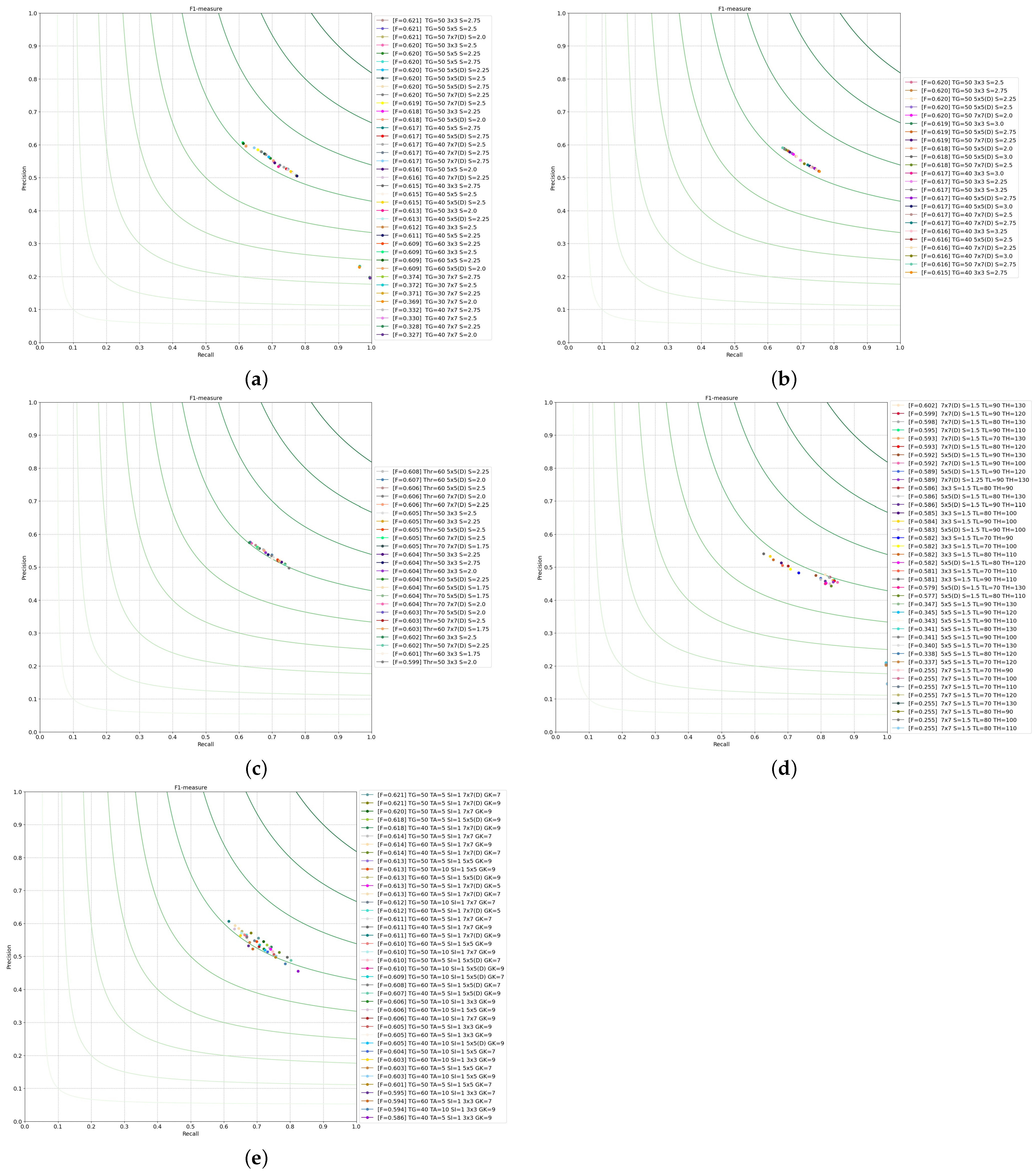
4. Experimental Results

In this section, we present the results of our analysis for each edge operator presented in Section 3. In our presentation, we provide visual results, statistical results and remarks for each subsection.

We attempt to prove the hypothesis that dilating the filters will cause better edge-detection results for each algorithm evaluated. To do so, we divide our evaluation into two sections: one evaluates the best versions (parameter configuration) of each edge operator using classical, extended or dilated kernels and the second evaluates if the trend results obtained in the first experiment are maintained if we change the kernels used with different ones found in the literature.

For our simulation to be reproducible and easy to use we have used the End-to-End Computer Vision Framework -EECVF- [73,74]. EECVF is an adaptable and dynamic framework designed for researching and testing CV concepts, which does not require the user to handle the interconnections throughout the system. All the edge operators and algorithms are present in the framework and can be reproduced by running the $main\_dilated\_filters\_for\_edge\_detection\_algorithms$ module.

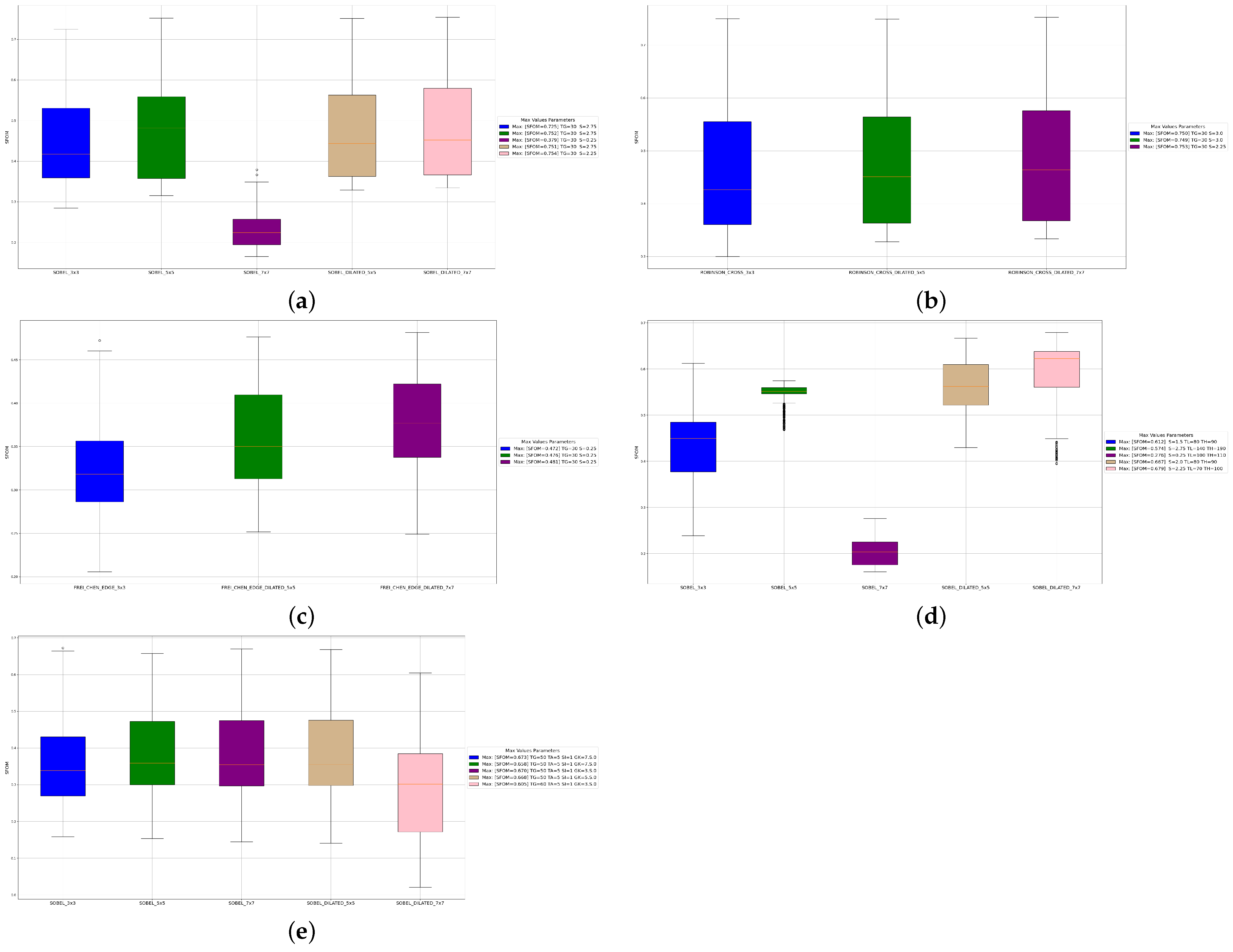
4.1. Effect of Dilation

In this Section, we analyze the hypothesis that dilating the filters yields better results than the original or expanded version. Because the topic of our evaluation is classical edge-detection algorithms, we have to take into account the direct effect of parameters over the resulting edge map. So we vary all the parameters (depending on the algorithm, see the details below) to find the best suited one for each variant. Because this parameter finding task results in a considerable number of variants, we only consider the best results for each variant that are evaluated with $BSDS500$. For the evaluation on the synthetic dataset, the results are presented in figures on this section. Due to the nature of the metrics used, in this case, we could consider a representation method that permits us to show all variants results.

In Figure 7 and Figure 8 we present the results for edge-detection operators that are based on first-order discrete kernels. As we can observe, we chose to vary the parameters for each version of the kernels (classic, extended or dilated) to obtain the best results we can with each one. For the edge operators presented in this figure, we have chosen the classical Sobel operator; for the first-order derivative compass Gradient we have used instead the Robinson Compass operator. An exception for this is the Frei-Chen algorithm that has a particular kernel.

In Figure 9 and Figure 10, we present the results of edge-detection operators that are based on second-order discrete kernels. For the edge operators presented in this figure, we have chosen the classical Laplace operator. For our simulation results and evaluation, we first searched for the best threshold value (see the interval searching details below) by using the Laplacian kernel V1 that we can find in Figure A4 from the Appendix A.

4.1.1. Operators Based on First-Order Discrete Kernels

In Figure 7a, we present the results for the first-order derivative orthogonal gradient operator. As we can observe, we have searched for the best $F1$ results in a range of the threshold between 30 and 160 with a step of 10 and sigma value between $0.25$ and $3.0$ with a step of $0.25$. As expected, a higher threshold will produce less edge points, as we can see in Figure A8, but with a fair confidence that resulted in a high R because of the lack of points. For the images, we use the following notations: Gaussian sigma is S and threshold is $TG$.

From the results presented in Figure 7a, we can observe that we obtain equal $F1$ scores for the 3 × 3 classical, 5 × 5 extended and 7 × 7 dilated kernel versions. On the other hand, we clearly see that expanding the kernel to 7 × 7 performs worse than dilation; the best results with 7 × 7 extensions were $0.374$.

In Figure 7b, we follow the $F1$ results for the first-order derivative compass gradient operators using some similar ranges of the threshold, between 30 and 160, and sigma value between $0.25$ and $3.5$. In the figure, we use the the same notations: Gaussian sigma is S and threshold is $TG$. In Figure 7b, we can notice that the 3 × 3 classical kernel obtains equal results similar to the 5 × 5 dilated or 7 × 7 dilated version. A notable difference in this case is the lack of extended kernels as they were not present in the literature.

The Frei–Chen operator is a special case of the compass gradient operators and is presented Section 3.4. We fine-tune the parameters of the algorithm for a range of the threshold between 30 and 160 and sigma value of the Gaussian filter blur between $0.25$ and $3.2$. The results are presented in Figure 7c, where we use the same notations: Gaussian sigma is S and threshold is $TG$. In this case with the Frei–Chen operator, the 7 × 7 dilated kernel version yields the best $F1$ results followed by the dilated 5 × 5 kernel. Similar to the compass gradient operators, an extension of this operator was not found in the literature for comparison.

One of the most popular first-order-derivative-based edge-detector operator is Canny, presented in Section 3.8. For parameter tuning, we varied the following configurations: Gaussian sigma value from $0.2$ to $3.0$ with a step of $0.25$, low threshold from 70 to 150 with a step of 10 and high threshold from 90 to 200 with a step of 10. We performed the parameter tuning phase for the original kernel, extended and dilated to find the best suited ones. For the images, we use the following notations: Gaussian sigma is S, low threshold is $TL$ and high threshold is $TH$.

For the ED algorithm, described in Section 3.10, we searched for the best combination of Gaussian smoothing kernel size, gradient threshold, anchor threshold and scan interval interval. We varied the parameters as follows: Gaussian kernel ($GK$) between 3 to 9 with a step of 2; gradient threshold ($TG$) between 10 and 150 with a step of 10; anchor threshold ($TA$) between 10 and 60 with a step of 10; scan interval ($SI$) in range of 1, 3, 5.

As we can see in Figure 7d,e, the best results we obtain were when using the 7 × 7 dilated filter. Another conclusion we draw is that using extended kernels will produce a significant degradation of the edge map results, supported by the lower score. An aspect worth mentioning for these two algorithms, Canny and ED, is the fact that for the ED algorithm, when using extended kernels, good results are obtained; it is also similar for the dilated 7 × 7 case. It is not the case for Canny, where the extension technique does not help anymore.

For the evaluation using $SFOM$, presented in Figure 8, we used the same parameter variation values in order to respect the same evaluation methodology.

From the results presented in Figure 8a, we can observe a clear degradation of the obtained edge map when considering the 7 × 7 extended kernel, with a maximum $SFoM$ value of $0.379$. When we look over the max peaks obtained when using 5 × 5, 7 × 7 dilated and 5 × 5, we observe that they are very close.

When looking over the results from the compass first-order operators, Figure 8b, we can observe similar max peaks but the median values increase directly with the dilatation factor.

In case of Frei–Chen edge operator, Figure 8c, we can observe a clear increase in the median values and max peak when using dilated kernels.

An interesting evolution can be observed in the case of the Canny algorithm, Figure 8d, where expanding the kernel to 5 × 5 brings benefits to the resulting edge map but expanding to 7 × 7 produces a significant degradation of the results. In case of dilating the kernels, improvements can be observed with the peak max values reaching up to $0.679$ for the 7 × 7 kernel.

The exception from the trend comes when talking about the ED algorithm, Figure 8e. In this case, expanding to 5 × 5 or dilating to 5 × 5 produces similar results ($0.658$ for expanding and $0.668$ for dilating). The difference occurs when looking at dilated 7 × 7 where we actually have a degradation of the results. The best results were actually obtained using the classical 3 × 3 with a value of $0.673$.

4.1.2. Operators Based on Second-Order Discrete Kernels

The Laplace edge operator is one of the most popular edge detectors based on second-order derivative discrete kernels, described in Section 3.5. We have chosen to vary the threshold from 15 to 245, the results can be observed in Figure 9a, where $TG$ is the notation of the threshold.

A natural extension of the Laplace operator is the Laplacian of Log, described in Section 3.6. We searched for the best combination of sigma for constructing the LoG kernel and the threshold. The results can be observed in Figure 9b. We have chosen to vary the threshold from 5 to 60, avoiding a bigger threshold. Bigger threshold values would not generate better results because of the small intensity resulted after the convolution. Regarding the sigma for the Gaussian blur kernel, we chose to vary between $0.2$ and $2.0$, while going higher would generate a lack of resulting edge points. For the images, we use the following notations: Gaussian sigma is S and threshold is $TG$.

Marr–Hildreth operator, presented in Section 3.7, is similar to the Log operator. We first searched the best combination of sigma for constructing the LoG kernel and the threshold of zero crossing. The results can be observed in Figure 9c and for a better visualization, we have chosen to show only the best results in $F1$ order. We have tried the combination of $sigma$ value from $0.2$ to $3.0$ with gradient threshold of 30 to 90 of the gradient image, considering that is the interval where these parameters bring good results to the output. For the images, we use the following notations: Gaussian sigma is S and threshold is $TG$.

The results and evaluation of Shen–Castan operator, described in Section 3.9, are presented in this section. We searched again for the best combination of threshold of Laplace, smoothing factor, window size, thinning factor and ratio factor of the algorithm. We chose a threshold value of 40 for the Laplace edge detector and vary the rest of the values as follows: smoothing factor of ISEF filter ($SF$) from $0.5$ to $0.9$; adaptive zero crossing window size (W) of 5, 7, 9; threshold for zero crossing (R) from $0.5$ to $0.9$; thinning factor ($TN$) of 0, $0.5$ and $0.9$.

There are multiple hyperparameter value combinations that yield the same $F1$ score. For example, the dilated 7 × 7 filter obtains an $F1$ score equal to $0.576$ for 4 different combinations of values for R and TN: $(TG=4,SF=0.9,W=11,R=0.5,TN=0),$$(TG=4,SF=0.9,W=11,R=0.5,TN=0.5),(TG=4,SF=0.9,W=11,$$R=0.9,$$TN=0),(TG=4,SF=0.9,W=11,R=0.5,TN=0.5)$.

Looking over the results from Figure 9a–d, we can observe that the best results were obtained using the 7 × 7 dilated version, followed by the 5 × 5 dilated version. We can also conclude that for this operator using the 5 × 5 extended kernel deteriorates the resulted edge map.

Similar to first-order-based algorithm, we chose to vary all the parameters in the same limits for these evaluation. These is important so we can correlate the results on the different datasets.

First we look over the results we obtained when evaluating the Laplace operator, see Figure 10a and we see that dilating bring forward significant improvements. We see a peak value of $0.478$ for 5 × 5 dilated and $0.470$ for 7 × 7.

If we look over the results from LoG operator, see Figure 10b, the dilatation produces slightly better results, but an interesting fact is the compression that we can see in the evaluation results interval.

In case of Marr–Hildreth, which can be seen in Figure 10c, the dilatation produces slightly increased max values, from $0.396$ for the 3 × 3 to $0.410$ for the 5 × 5 dilated. We can observe in the opposite part a decrease in evaluation results in case of the 5 × 5 version.

In the Shen–Castan results presented in Figure 10d, we detect a clear improvement when using dilated kernels. The max values are obtained when we use the 5 × 5 dilated version: $0.442$, whereas the classical version obtains $0.315$.

As a conclusion from the evaluation of second-order-based operators using $SFOM$, we can clearly see that using 5 × 5 dilated yield better results in the edge map.

4.1.3. Preliminary Conclusion

In

Table 1. Overall best results for each edge operator analyzed.

Operator	PCM [69]					SFOM [58]
	Kernel	P	R	F1	Parameters	Kernel	SFoM	Parameters
First Order Orthogonal	7 × 7(D)	0.571	0.679	0.621	TG = 50, S = 2.75	7 × 7(D)	0.754	TG = 30, S = 2.25
First Order Compass	5 × 5(D)	0.565	0.687	0.620	TG = 50, S = 2.25	7 × 7(D)	0.753	TG = 30, S = 2.25
Frei–Chen	5 × 5(D)	0.554	0.673	0.608	TG = 60, S = 2.25	7 × 7(D)	0.481	TG = 30, S = 0.25
Laplace	7 × 7(D)	0.309	0.794	0.445	TG = 95	5 × 5(D)	0.478	TG = 15
LoG	7 × 7(D)	0.490	0.659	0.562	TG = 30, S = 1.8	7 × 7(D)	0.491	TG = 5, S = 1.0
Marr–Hildreth	7 × 7(D)	0.450	0.744	0.561	TG = 0.2, S = 2.0	5 × 5(D)	0.411	TG = 0.2, S = 1.6
Canny	7 × 7(D)	0.478	0.813	0.602	S = 1.5, TL = 90, TH = 130	7 × 7(D)	0.679	S = 2.25, TL = 70, TH = 100
Shen–Castan	7 × 7(D)	0.483	0.711	0.576	TG = 4, SF = 0.9, W = 11, TN = 0	5 × 5(D)	0.442	TG = 4, SF = 0.9, W = 11, TN = 0.5
ED	7 × 7(D)	0.556	0.704	0.621	TG = 50, TA = 5, SI = 1, GK = 7	3 × 3	0.673	TG = 50, TA = 5, SI = 1, GK = 7

, we present for each edge operator the best results we could obtain and also specify the kernel that was used. From our experiments, we can conclude that for all edge-detection operators, using the dilated version of the kernels has a positive effect upon the resulting edge map when evaluating using $PCM$ on $BSDS500$. When looking over the evaluation using $SFoM$, we observe that we obtained better results when we used the dilated kernels, with the exception of the ED algorithm.

The exception we have for the first-order derivative orthogonal gradient operators and first-order derivative compass gradient operators was that the 7 × 7 dilated version of the kernels obtained the same $F1$ score as the classical 3 × 3 ones. We chose to use the dilated because of the higher p value.

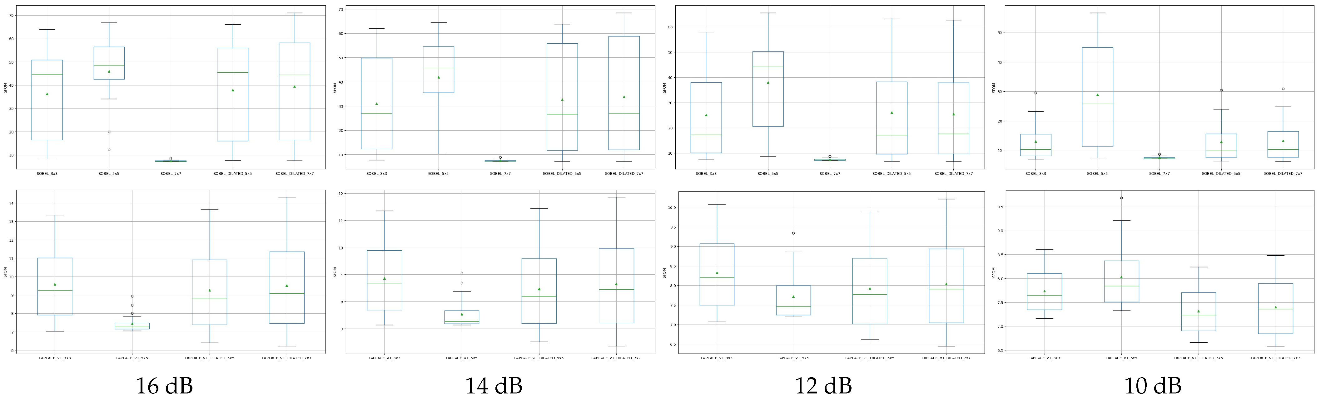
4.2. Noise Effect on Dilation

Edge detection algorithms have a different sensitivity regarding the noise level of the input image. In this section, we analyze the effect that the addition noise had upon the resulting edge map, when using a dilated filter. To do so, we used an image from the synthetic dataset [12] and applied it to different levels of noise (Gaussian noise) at various peak signal-to-noise ratio ($\mathrm{PSNR}$) values (from 16 dB to 10 dB), see Figure 11.

In order to have a complete evaluation of the dilated filter impact, we conducted similar experiments for noise sensibility analysis, as was presented in [58,59,75]. To maintain consistency in our evaluation, we used the two algorithms presented in Section 3. For each image with different noise levels, we varied the algorithm parameter as we described in Section 4.1; however, we evaluated them using the $SFoM$ measure. We chose the first-order derivative orthogonal gradient algorithm as we consider it to be the most sensitive to noise from the first-order derivative group. Similar to the second-order derivative group, we chose the Laplace operator. In order to have a more objective analysis we have eliminated the smoothing step from the first-order gradient, see Algorithm 2. Further, for a complete evaluation of the dilated filter impact we conduct similar methodology for noise sensibility analysis, as was presented in [58,59]. In Figure 12, we highlighted the visual results obtained for first-order gradient algorithm. In the first row are the filtered images without any noise, for 3, 5, 7, dilated 5 and dilated 7 filters. For each new row the noise increases from 16 dB to 10 dB. We can observe that dilation is not that sensible for noise, and requires statistical analysis.

Interpreting the statistical results that we obtained in Figure 13, one can observe that the noise has the same effect upon the classical or dilated versions of the filters. We can observe as the noise level is growing the median and maximum value of the $SFoM$ decreases. For the first-order derivative orthogonal gradient operator, the noise does not have a huge impact over our dilated proposed approach. From the left to right, with the noise increasing, it is normal to obtain some degradation; however, the classical Sobel $3\times 3$ or the extension obtained the same degradation. With all the noises, the dilated filters are above the classical methods in performance, even in the average or mean of the results.

In the second line of Figure 13, we present the statistical results of the second derivative operator. We can see that noise has the same impact in the classical Laplace results and for our dilated filter approach. What is worth mentioning in both cases, Sobel and Laplace, is that $5\times 5$ extended seems that it is increasing, but looking closer to the $SFOM$ values, we can observe that it actually has a stable variant (e.g., is always between 7 and 8 on the second order).

The more complex algorithms that are presented in this paper are extensions or improvements of one of the two algorithms. In this case, we consider that extending our analysis will not bring considerable improvements. We can conclude that the noise level affects the classical and dilated filters to the same extent.

4.3. Dilation with Different Operators

In this Section, we analyze if the hypothesis that dilating the filters yields better results than the classical approach is maintained if we change the kernel used. In Figure 14, we present the results for edge-detection operators that are based on first-order discrete kernels and in Figure 15, we present the results of edge-detection operators that are based on second-order discrete kernels. From the previous results, because both metrics showed similar conclusions, we consider in the next part of this paper, only the $BSDS500$ dataset evaluation.

For each version of the kernel (classical, extended or dilated) we used the best-suited parameters found in Section 4 for this evaluation. Statistical metrics are presented in Figure 14 and Figure 15 and visual comparison results of the operators are presented in Figure A8, Figure A9, Figure A10, Figure A11 and Figure A12 from Appendix B.

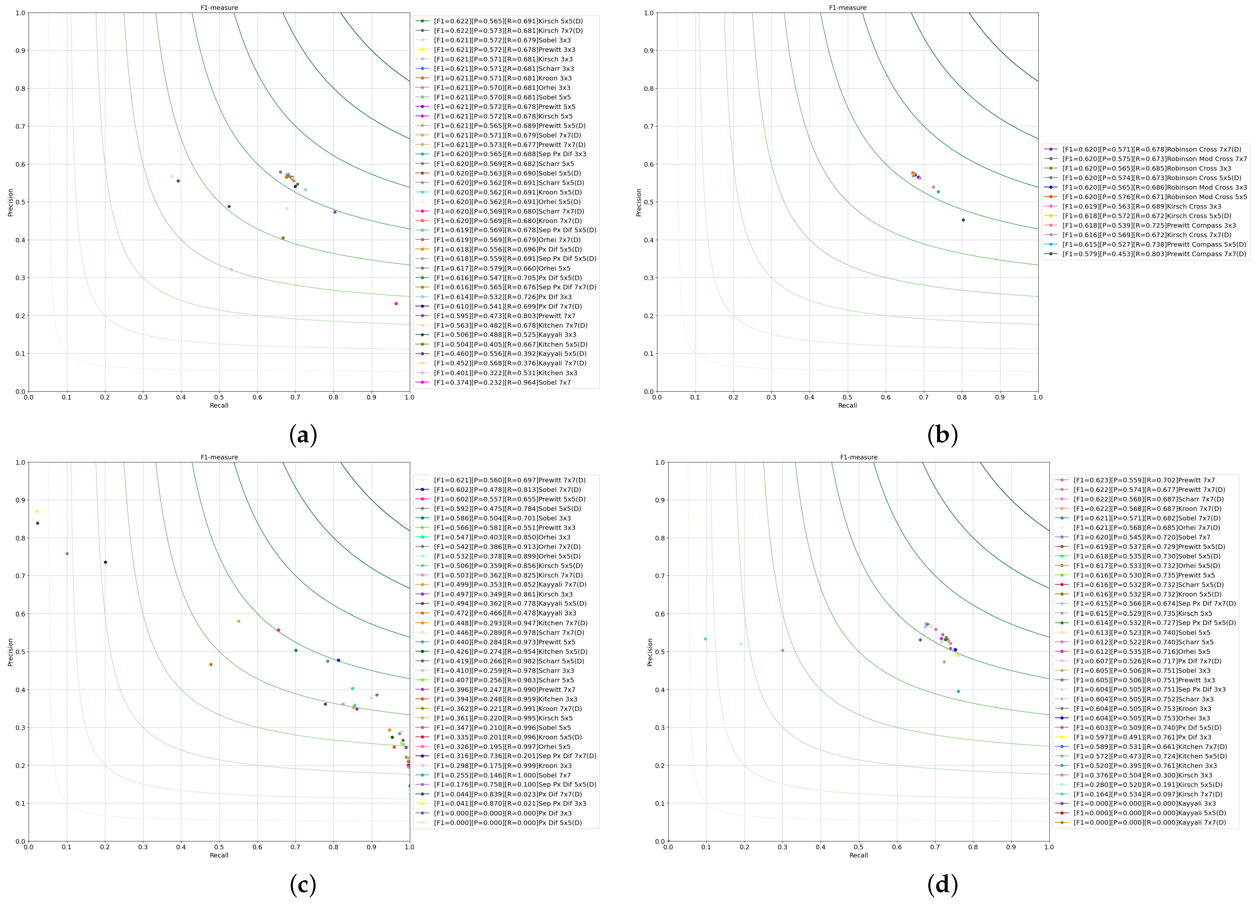
4.3.1. Operators Based on First-Order Discrete Kernels

For this section, we alter the classical Sobel kernel with the following filters: pixel difference operator, separated pixel difference operator, Sobel operator, Prewitt operator, Kirsch operator, Kitchen and Malin operator, Kayalli operator, Scharr operator, Kroon operator and Orhei operator.

For the first-order derivative compass gradient operators, we found in the literature the following: Prewitt compass operator, Robinson compass operator and Kirsch compass operator. For this section, we do not consider the Frei–Chen operator where the kernel is fixed. Analyzing the effect of changing the kernel is not the focus of this research.

The first aspect worth mentioning for Figure 14 is that for each algorithm, the best results were obtained when using dilated versions of the kernels. Another important aspect is that in most cases, even if we change the kernel we obtain the same trend, which is that dilation obtains better results.

For the first-order derivative orthogonal gradient operators, Figure 14a, we observe that using the Kirsch operator obtains good results in all cases classical, extended or dilated. In the opposite part, we have the Kayyali operator, where dilating the filters produced a degradation of the resulting edge map.

In Figure 14b, we present the results for the first-order derivative compass gradient operators, where we observe that for both variants of the Robinson compass operator, we obtained similar results if we use the classical or dilated approach. Unfortunately, we can see clear diminution of the $F1$ metric when dilating using Prewitt compass operator.

In the case of the Canny operator, Figure 14c, we see that the trend we observed for the Sobel operator is maintained for most of the other operators we experimented with. We consider it worth mentioning that we used the dilated 7 × 7 Prewitt operator, and we see a significant increase in the overall results. In the case of this algorithm, we actually observed that the pixel difference operator and separated pixel difference operator do not obtain any noticeable results.

In Figure 14d, we can see that, for the ED algorithm, we obtained the same close results for the dilated 7 × 7 and extended 7 × 7 for several operators, such as: Sobel, Kroon, Prewitt and Orhei. Actually, in this case, the first results were where the extended kernels produced the best overall results. On the other hand, we can conclude that the Kayyali operator has no benefit when it is used in this algorithm.

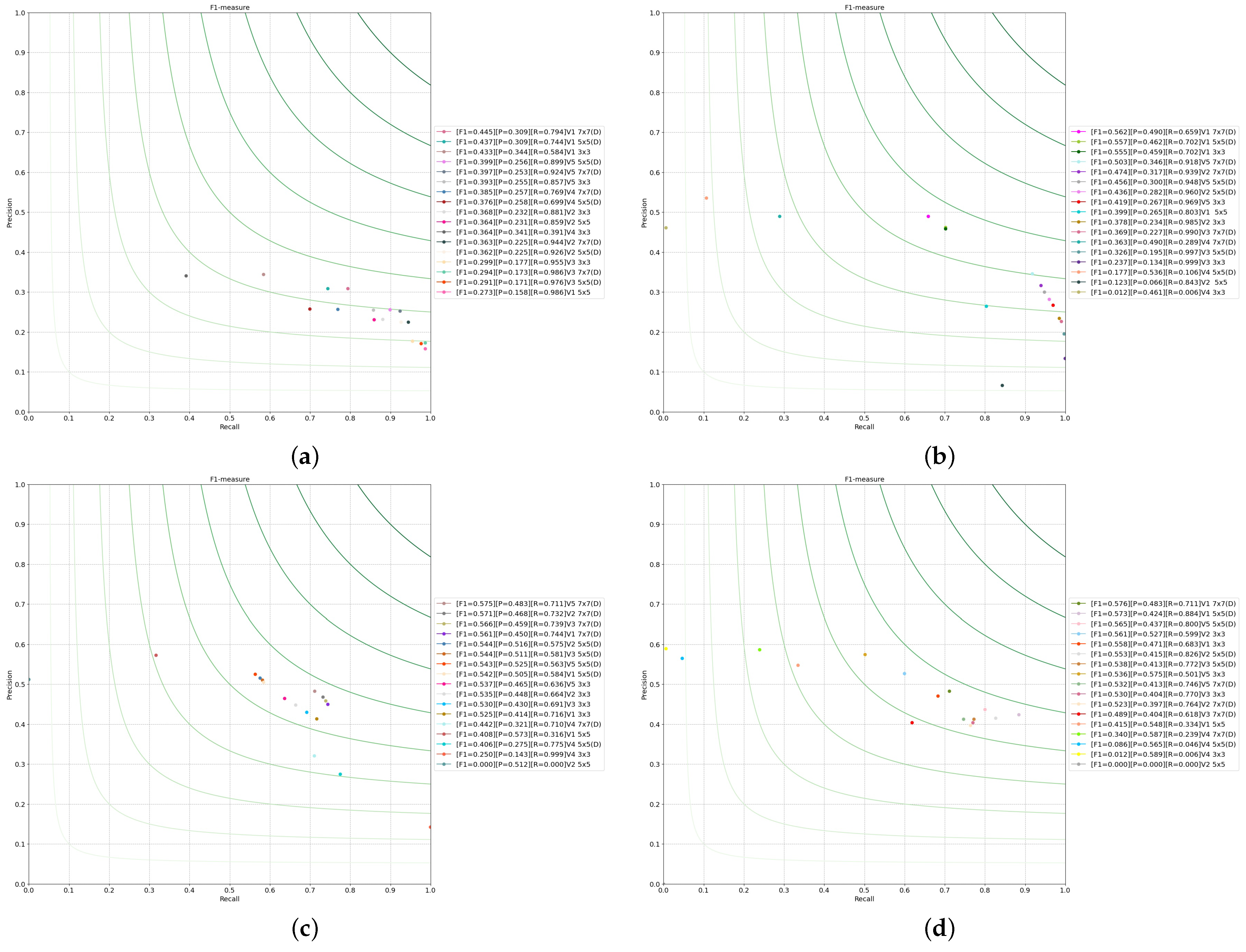
4.3.2. Operators Based on Second-Order Discrete Kernels

For this section, we change the classical Laplace kernel with the alternative approximations we found in the literature; see Figure A4 and Figure A5 in Appendix A.

The first aspect worth mentioning for Figure 15 is that, for each algorithm, the best results were obtained when using dilated 7 × 7 versions of the kernels. Another important aspect is that in most cases even if we change the kernel we obtained better results with dilation.

For the Laplace operator, Figure 15a, we can observe that in the case of kernels $V1$, $V4$ and $V5$ we have the same trend for the top three in the results: classic 3 × 3, dilated 5 × 5 and the best dilated 7 × 7; however, we have to mention that for the $V3$ and $V2$ the best results were obtained with the classical approaches.

In Figure 15b, where we see the results for the LoG algorithm, we can conclude that for all versions of the kernels, we obtained better results for the dilated versions. This trend is maintained for the Marr–Hildreth algorithm as presented in Figure 15c.

For the Shen–Castan algorithm, we obtained another exception from the trend we observed in the case of kernels $V2$ and $V3$; see Figure 15d. Similar to the other algorithm, we obtained the worst metrics for the 5 × 5 extended version of the kernels.

4.3.3. Preliminary Conclusion

By analyzing the results obtained in this section, see Figure 14 and Figure 15, we find that in most cases, even if we changed the kernel used, we obtained better results when we dilated the kernels. As expected, changing the operators we used has an effect on the resulting edge map but not in the trend of the results (performance of classic, extended or dilated).

5. Conclusions and Future Work

In this paper, we extend our work (see the previous papers [11,12]) regarding dilation of a classical convolution edge-detection filters. In Section 3, we present the theoretical background where we present the algorithms that took part in the simulation from Section 4. The experimental results confirm our hypothesis that the dilation of filters have a positive impact for edge detection.

From the summary made in Table 1, we can state that the dilated filter yields, generally speaking, better results. This hypothesis was proven using two different metrics, $PCM$ and $SFoM$, on two different datasets. The evaluation that we performed helped us demonstrate the initial hypothesis that the dilation of the kernels leads to edge-detection improvements.

Dilating first-order derivative kernels yields results similar to the classical 3 × 3 kernel in the worst case, and sometimes significant improvements in the best case, as we can see in Figure 7d or Figure 8d. When experimenting with different kernels, we observed that the respective trends in terms of the results is maintained, see Figure 14.

Dilating the second-order discrete approximation filter did yield considerable improvements to the edge map, as we see in Figure 9c when using the Marr–Hildreth algorithm or in Figure 9d for the Shen–Castan algorithm. When we experimented with different Laplace kernels, we observed the same behavior except with a reduced number of cases such as $V3$ in the case of Laplace operator; see Figure 15a. When evaluating with the $SFoM$ metric, we observed improvements overall when using the 5 × 5 dilated kernels as we can see Figure 10a–d.

Statistically and visually, we could observe that by dilating the filters we find more edge pixels than by the classical operators. By dilation, we obtained a better precision and $F1$-score, which can be observed in the results we presented. By the simple structure of the dilated filters, they are also a good choice when the runtime matters. The other classical filter extensions from [33,35,36,37,40] require a larger number of operations in order to return the resulting edge pixels, whereas the custom dilated filters always have the same number of operations for any extension. It seems that the gaps imply a speed up. We can point out that, for the ED algorithm, see Figure 14d, we have obtained the best results when using the 7 × 7 kernel with the Prewitt kernel.

In Section 4.2, we explored the effect of noise on the dilated filter and concluded that it has a similar effect as in classical filters. We may, in our future work, continue this analysis of the dilated-threshold-noise effect by using different metrics, such as the minimum score proposed by [59].

In our research, we focused on dilating 3 × 3 filters, but in our future work, we will concern ourselves in dilating bigger kernels as a starting point. This can be analyzed from the definition of the dilation. Another aspect worth exploring in the future would be to run experiments in automated threshold versions of the algorithms. Our current experiments focused on the classical version of edge-detection algorithms, but looking into the combined effects of dilating and automated threshold could enhance the resulted edge map.

In our approach, for comparison purposes, the focus was to fine-tune the classical edge-detection algorithms in order to obtain the optimal threshold and sigma values. We are certain that if we would have fine-tuned the algorithms for the dilated kernel, the results would have been better.

In general we can state that using the dilated kernels yields benefits regarding the edge map, as a result of the edge-detection of the classical algorithm and the run-time needed. We obtained similar or better results when taking into consideration a bigger neighborhood.

References

1. Ziou, D.; Tabbone, S. Edge detection techniques-an overview. Pattern Recognit. Image Anal. C/C Raspoznavaniye Obraz. Anal. Izobr. 1998, 8, 537–559. [Google Scholar]
2. Papari, G.; Petkov, N. Edge and line oriented contour detection: State of the art. Image Vis. Comput. 2011, 29, 79–103. [Google Scholar] [CrossRef]
3. Spontón, H.; Cardelino, J. A review of classic edge detectors. Image Process. Line 2015, 5, 90–123. [Google Scholar] [CrossRef] [Green Version]
4. Sen, D.; Pal, S.K. Gradient histogram: Thresholding in a region of interest for edge detection. Image Vis. Comput. 2010, 28, 677–695. [Google Scholar] [CrossRef]
5. Haralick, R.M.; Shapiro, L.; Lee, J. Morphological edge detection. IEEE J. Robot. Autom. 1987, 3, 142–155. [Google Scholar]
6. Hamaguchi, R.; Fujita, A.; Nemoto, K.; Imaizumi, T.; Hikosaka, S. Effective Use of Dilated Convolutions for Segmenting Small Object Instances in Remote Sensing Imagery. In Proceedings of the 2018 IEEE Winter Conference on Applications of Computer Vision, WACV 2018, Lake Tahoe, NV, USA, 12–15 March 2018; pp. 1442–1450. [Google Scholar] [CrossRef] [Green Version]
7. Chen, L.; Papandreou, G.; Kokkinos, I.; Murphy, K.; Yuille, A.L. DeepLab: Semantic Image Segmentation with Deep Convolutional Nets, Atrous Convolution, and Fully Connected CRFs. IEEE Trans. Pattern Anal. Mach. Intell. 2018, 40, 834–848. [Google Scholar] [CrossRef] [PubMed]
8. Yazdanbakhsh, O.; Dick, S. Multivariate Time Series Classification using Dilated Convolutional Neural Network. arXiv 2019, arXiv:1905.01697. [Google Scholar]
9. Yu, F.; Koltun, V. Multi-Scale Context Aggregation by Dilated Convolutions. In Proceedings of the 4th International Conference on Learning Representations, ICLR 2016, San Juan, PR, USA, 2–4 May 2016; Conference Track Proceedings. Bengio, Y., LeCun, Y., Eds.; ICLR: San Juan, PR, USA, 2016. [Google Scholar]
10. Zhao, H.; Shi, J.; Qi, X.; Wang, X.; Jia, J. Pyramid Scene Parsing Network. In Proceedings of the 2017 IEEE Conference on Computer Vision and Pattern Recognition, CVPR 2017, Honolulu, HI, USA, 21–26 July 2017; pp. 6230–6239. [Google Scholar] [CrossRef] [Green Version]
11. Bogdan, V.; Bonchiş, C.; Orhei, C. Custom Dilated Edge Detection Filters. J. WSCG 2020, 28, 161–168. [Google Scholar] [CrossRef]
12. Orhei, C.; Bogdan, V.; Bonchiş, C. Edge map response of dilated and reconstructed classical filters. In Proceedings of the 2020 22nd International Symposium on Symbolic and Numeric Algorithms for Scientific Computing (SYNASC), Timisoara, Romania, 1–4 September 2020; pp. 187–194. [Google Scholar] [CrossRef]
13. Canny, J. A Computational Approach to Edge Detection. IEEE Trans. Pattern Anal. Mach. Intell. 1986, PAMI-8, 679–698. [Google Scholar] [CrossRef]
14. Sobel, I.; Feldman, G. A 3 × 3 isotropic gradient operator for image processing. Pattern Classif. Scene Anal. 1973, 271–272, unpublished. [Google Scholar]
15. Prewitt, J.M. Object enhancement and extraction. Pict. Process. Psychopictorics 1970, 10, 15–19. [Google Scholar]
16. Scharr, H. Optimal Operators in Digital Image Processing. Ph.D. Thesis, University of Heidelberg, Heidelberg, Germany, 2000. [Google Scholar]
17. Marr, D.; Hildreth, E. Theory of edge detection. Proc. R. Soc. Lond. Ser. Biol. Sci. 1980, 207, 187–217. [Google Scholar]
18. Castan, S.; Zhao, J.; Shen, J. New edge detection methods based on exponential filter. In Proceedings of the 10th International Conference on Pattern Recognition, Atlantic City, NJ, USA, 16–21 June 1990; Volume 1, pp. 709–711. [Google Scholar] [CrossRef]
19. Chen, C.C. Fast boundary detection: A generalization and a new algorithm. IEEE Trans. Comput. 1977, 100, 988–998. [Google Scholar]
20. Park, R.H. A Fourier interpretation of the Frei-Chen edge masks. Pattern Recognit. Lett. 1990, 11, 631–636. [Google Scholar] [CrossRef]
21. Topal, C.; Akinlar, C. Edge drawing: A combined real-time edge and segment detector. J. Vis. Commun. Image Represent. 2012, 23, 862–872. [Google Scholar] [CrossRef]
22. Jain, R.; Kasturi, R.; Schunck, B.G. Machine Vision; McGraw-hill: New York, NY, USA, 1995; Volume 5. [Google Scholar]
23. Haralick, R.M.; Shapiro, L.G. Computer and Robot Vision; Addison-Wesley Reading: Boston, MA, USA, 1992; Volume 1. [Google Scholar]
24. Liu, H.; Jezek, K. Automated extraction of coastline from satellite imagery by integrating Canny edge detection and locally adaptive thresholding methods. Int. J. Remote Sens. 2004, 25, 937–958. [Google Scholar] [CrossRef]
25. Isa, N.M. Automated edge detection technique for Pap smear images using moving K-means clustering and modified seed based region growing algorithm. Int. J. Comput. Internet Manag. 2005, 13, 45–59. [Google Scholar]
26. Orhei, C.; Mocofan, M.; Vert, S.; Vasiu, R. An automated threshold Edge Drawing algorithm. In Proceedings of the 2021 44th International Conference on Telecommunications and Signal Processing (TSP), Brno, Czech Republic, 26–28 July 2021; pp. 292–295. [Google Scholar] [CrossRef]
27. Jie, G.; Ning, L. An improved adaptive threshold canny edge detection algorithm. In Proceedings of the 2012 International Conference on Computer Science and Electronics Engineering, Hangzhou, China, 23–25 March 2012; Volume 1, pp. 164–168. [Google Scholar]
28. Azeroual, A.; Afdel, K. Fast image edge detection based on faber schauder wavelet and otsu threshold. Heliyon 2017, 3, e00485. [Google Scholar] [CrossRef] [Green Version]
29. Xu, Q.; Chakrabarti, C.; Karam, L.J. A distributed Canny edge detector and its implementation on FPGA. In Proceedings of the 2011 Digital Signal Processing and Signal Processing Education Meeting (DSP/SPE), Sedona, AZ, USA, 4–7 January 2011; pp. 500–505. [Google Scholar]
30. Sezgin, M.; Sankur, B. Survey over image thresholding techniques and quantitative performance evaluation. J. Electron. Imaging 2004, 13, 146–165. [Google Scholar]
31. Guo, Z.; Hall, R.W. Parallel thinning with two-subiteration algorithms. Commun. ACM 1989, 32, 359–373. [Google Scholar] [CrossRef]
32. Mlsna, P.A.; Rodriguez, J.J. Gradient and Laplacian edge detection. In The Essential Guide to Image Processing; Elsevier: Amsterdam, The Netherlands, 2009; pp. 495–524. [Google Scholar]
33. Bandai, N.; Sanada, S.; Ueki, K.; Funabasama, S.; Tsuduki, S.; Matsui, T. Morphological analysis for kinetic X-ray images of the temporomandibular joint. Nihon Hoshasen Gijutsu Gakkai Zasshi 2003, 59, 951. [Google Scholar] [CrossRef] [PubMed] [Green Version]
34. Lateef, R.A.R. Expansion and Implementation of a 3 × 3 Sobel and Prewitt Edge Detection Filter to a 5 × 5 Dimension Filter. J. Baghdad Coll. Econ. Sci. Univ. 2008, 1, 336–348. [Google Scholar]
35. Kekre, H.; Gharge, S. Image Segmentation using Extended Edge Operator for Mammographic Images. Int. J. Comput. Sci. Eng. 2010, 2, 1086–1091. [Google Scholar]
36. Levkine, G. Prewitt, Sobel and Scharr gradient 5 × 5 convolution matrices. Image Process. Artic. Second. Draft 2012. Available online: http://www.hlevkin.com/articles/SobelScharrGradients5x5.pdf (accessed on 9 November 2021).
37. Gupta, S.; Mazumdar, S.G. Sobel edge detection algorithm. Int. J. Comput. Sci. Manag. Res. 2013, 2, 1578–1583. [Google Scholar]
38. Kirsch, R.A. Computer determination of the constituent structure of biological images. Comput. Biomed. Res. 1971, 4, 315–328. [Google Scholar] [CrossRef]
39. Kitchen, L.; Malin, J. The effect of spatial discretization on the magnitude and direction response of simple differential edge operators on a step edge. Comput. Vis. Graph. Image Process. 1989, 47, 243–258. [Google Scholar] [CrossRef]
40. Chen, J.; Chen, D.; Meng, S. A Novel Region Selection Algorithm for Auto-focusing Method Based on Depth from Focus. In Proceedings of the Euro-China Conference on Intelligent Data Analysis and Applications, Málaga, Spain, 9–11 October 2017; Springer: Berlin/Heidelberg, Germany, 2017; pp. 101–108. [Google Scholar]
41. Kroon, D. Numerical Optimization of Kernel Based Image Derivatives; Short Paper University Twente: Enschede, The Netherlands, 2009. [Google Scholar]
42. Orhei, C.; Vert, S.; Vasiu, R. A Novel Edge Detection Operator for Identifying Buildings in Augmented Reality Applications. In Proceedings of the International Conference on Information and Software Technologies, Kaunas, Lithuania, 15–17 October 2020; pp. 208–219. [Google Scholar] [CrossRef]
43. Woods, J.W. Multidimensional Signal, Image, and Video Processing and Coding, Second Edition, 2nd ed.; Academic Press, Inc.: Orlando, FL, USA, 2011. [Google Scholar]
44. Gonzalez, C.; Woods, E. Digital Image Processing; Addison-Wesley Publishing Company: Boston, MA, USA, 1991. [Google Scholar]
45. Szeliski, R. Computer Vision: Algorithms and Applications; Springer Science & Business Media: Berlin/Heidelberg, Germany, 2010. [Google Scholar]
46. Robinson, G.S. Edge detection by compass gradient masks. Comput. Graph. Image Process. 1977, 6, 492–501. [Google Scholar] [CrossRef]
47. Davies, E. A skimming technique for fast accurate edge detection. Signal Process. 1992, 26, 1–16. [Google Scholar] [CrossRef]
48. Torre, V.; Poggio, T.A. On edge detection. IEEE Trans. Pattern Anal. Mach. Intell. 1986, PAMI-8, 147–163. [Google Scholar] [CrossRef]
49. Haralick, R.M. Digital Step Edges from Zero Crossing of Second Directional Derivatives. In Readings in Computer Vision; Fischler, M.A., Firschein, O., Eds.; Morgan Kaufmann: San Francisco, CA, USA, 1987; pp. 216–226. [Google Scholar] [CrossRef]
50. Grimson, W.E.L.; Hildreth, E.C. Comments on Digital Step Edges from Zero Crossings of Second Directional Derivatives. IEEE Trans. Pattern Anal. Mach. Intell. 1985, PAMI-7, 121–127. [Google Scholar] [CrossRef] [PubMed]
51. Parker, J.R. Algorithms for Image Processing and Computer Vision; John Wiley & Sons: Hoboken, NJ, USA, 2010. [Google Scholar]
52. Li, Z.; Aberkane, A.; Magnier, B. Shen-Castan Based Edge Detection Methods for Bayer CFA Images. In Proceedings of the 2021 9th European Workshop on Visual Information Processing (EUVIP), Paris, France, 23–25 June 2021; pp. 1–6. [Google Scholar]
53. Shen, J.; Castan, S. An optimal linear operator for step edge detection. CVGIP Graph. Model. Image Process. 1992, 54, 112–133. [Google Scholar] [CrossRef]
54. Aurich, V.; Weule, J. Non-linear gaussian filters performing edge preserving diffusion. In Mustererkennung 1995; Springer: Berlin/Heidelberg, Germany, 1995; pp. 538–545. [Google Scholar]
55. Wang, S.; Ge, F.; Liu, T. Evaluating edge detection through boundary detection. EURASIP J. Adv. Signal Process. 2006, 2006, 1–15. [Google Scholar] [CrossRef] [Green Version]
56. Kitchen, L.; Rosenfeld, A. Edge evaluation using local edge coherence. IEEE Trans. Syst. Man Cybern. 1981, 11, 597–605. [Google Scholar] [CrossRef]
57. Heath, M.D.; Sarkar, S.; Sanocki, T.; Bowyer, K.W. A robust visual method for assessing the relative performance of edge-detection algorithms. IEEE Trans. Pattern Anal. Mach. Intell. 1997, 19, 1338–1359. [Google Scholar] [CrossRef] [Green Version]
58. Magnier, B. Edge detection: A review of dissimilarity evaluations and a proposed normalized measure. Multimed. Tools Appl. 2018, 77, 9489–9533. [Google Scholar] [CrossRef] [Green Version]
59. Magnier, B.; Abdulrahman, H.; Montesinos, P. A review of supervised edge detection evaluation methods and an objective comparison of filtering gradient computations using hysteresis thresholds. J. Imaging 2018, 4, 74. [Google Scholar] [CrossRef] [Green Version]
60. Yitzhaky, Y.; Peli, E. A method for objective edge detection evaluation and detector parameter selection. IEEE Trans. Pattern Anal. Mach. Intell. 2003, 25, 1027–1033. [Google Scholar] [CrossRef]
61. Arbelaez, P.; Maire, M.; Fowlkes, C.; Malik, J. Contour Detection and Hierarchical Image Segmentation. IEEE Trans. Pattern Anal. Mach. Intell. 2011, 33, 898–916. [Google Scholar] [CrossRef] [Green Version]
62. Sun, W.; You, S.; Walker, J.; Li, K.; Barnes, N. Structural Edge Detection: A Dataset and Benchmark. In Proceedings of the 2018 Digital Image Computing: Techniques and Applications (DICTA), Canberra, Australia, 10–13 December 2018; pp. 1–8. [Google Scholar] [CrossRef]
63. Mély, D.A.; Kim, J.; McGill, M.; Guo, Y.; Serre, T. A systematic comparison between visual cues for boundary detection. Vis. Res. 2016, 120, 93–107. [Google Scholar] [CrossRef]
64. Silberman, N.; Hoiem, D.; Kohli, P.; Fergus, R. Indoor Segmentation and Support Inference from RGBD Images. In Proceedings of the European Conference on Computer Vision, Florence, Italy, 7–13 October 2012. [Google Scholar] [CrossRef]
65. Soria, X.; Riba, E.; Sappa, A. Dense Extreme Inception Network: Towards a Robust CNN Model for Edge Detection. In Proceedings of the IEEE/CVF Winter Conference on Applications of Computer Vision, Snowmass Village, CO, USA, 1–5 March 2020. [Google Scholar]
66. Orhei, C.; Vert, S.; Mocofan, M.; Vasiu, R. TMBuD: A dataset for urban scene building detection. In Proceedings of the International Conference on Information and Software Technologies, Kaunas, Lithuania, 14–16 October 2021; pp. 251–262. [Google Scholar] [CrossRef]
67. Orhei, C.; Mocofan, M.; Vert, S.; Vasiu, R. An analysis of ED line algorithm in urban street-view dataset. In Proceedings of the International Conference on Information and Software Technologies, Kaunas, Lithuania, 14–16 October 2021; pp. 123–135. [Google Scholar] [CrossRef]
68. Guizhen, M.; Zongliang, F.; Zongzhong, Y. Performance analysis and comparison of susan edge detector. Mod. Electron. Tech. 2007, 8, 189–191. [Google Scholar]
69. Prieto, M.; Allen, A. A similarity metric for edge images. Pattern Anal. Mach. Intell. IEEE Trans. 2003, 25, 1265–1273. [Google Scholar] [CrossRef]
70. Sasaki, Y. The Truth of the F-Measure; Technical Report; School of Computer Science, University of Manchester: Oxford, UK, 2007. [Google Scholar]
71. Abdou, I.; Pratt, W. Quantitative design and evaluation of enhancement/thresholding edge detectors. Proc. IEEE 1979, 67, 753–763. [Google Scholar] [CrossRef]
72. Dubuisson, M.P.; Jain, A.K. A modified Hausdorff distance for object matching. In Proceedings of the 12th International Conference on Pattern Recognition, Jerusalem, Israel, 9–13 October 1994; Volume 1, pp. 566–568. [Google Scholar]
73. Orhei, C.; Mocofan, M.; Vert, S.; Vasiu, R. End-to-End Computer Vision Framework. In Proceedings of the 2020 International Symposium on Electronics and Telecommunications (ISETC), Timisoara, Romania, 5–6 November 2020; pp. 1–4. [Google Scholar] [CrossRef]
74. Orhei, C.; Vert, S.; Mocofan, M.; Vasiu, R. End-To-End Computer Vision Framework: An Open-Source Platform for Research and Education. Sensors 2021, 21, 3691. [Google Scholar] [CrossRef] [PubMed]
75. Isar, A.; Nafornita, C.; Magu, G. Hyperanalytic Wavelet-Based Robust Edge Detection. Remote Sens. 2021, 13, 2888. [Google Scholar] [CrossRef]
Figure 1. Example of edge map results using Canny algorithm configured with the same parameters. Columns are: Original image; Canny using 3 × 3 kernel; Canny using dilated 5 × 5 kernel; Canny using dilated 7 × 7 kernel.
Applsci 11 10716 g001
Figure 2. Example of edge map results using Canny algorithm configured with different parameters. Columns are the low and high threshold combinations used: (20, 60); (50, 90); (70, 110); (90, 130); (110, 150); (130, 170); (150, 190). Rows represent the filter used: 3 × 3 filter edge; 5 × 5 dilated filter; 7 × 7 dilated filter.
Applsci 11 10716 g002
Figure 3. General kernel dilated with different factors.
Applsci 11 10716 g003
Figure 4. (a) 3 × 3 window showing 8-neighborhood of a pixel; (b) 4-connectivity; (c) 8-connectivity.
Applsci 11 10716 g004
Figure 5. Example of images and corresponding ground truth from B S D S 500 .
Applsci 11 10716 g005
Figure 6. Synthetic gray-scale test images (ae).
Applsci 11 10716 g006
Figure 7. Best results on B S D S 500 for classic, extended and dilated using different parameters for: (a) first-order derivative orthogonal gradient operators; (b) first-order derivative compass gradient operators; (c) Frei–Chen edge operator; (d) Canny operator; (e) ED edge operator.
Applsci 11 10716 g007
Figure 8. Best results on the synthetic dataset for classic, extended and dilated using different parameters for: (a) first-order derivative orthogonal gradient operators; (b) first-order derivative compass gradient operators; (c) Frei–Chen edge operator; (d) Canny operator; (e) ED edge operator.
Applsci 11 10716 g008
Figure 9. Finding the best results for classic, extended and dilated using different parameters for: (a) Laplace edge operator; (b) LoG edge operator; (c) Marr–Hildreth edge operator; (d) Shen–Castan edge operator.
Applsci 11 10716 g009
Figure 10. Finding the best results for classic, extended and dilated using different parameters for: (a) Laplace edge operator; (b) LoG edge operator; (c) Marr–Hildreth edge operator; (d) Shen–Castan edge operator.
Applsci 11 10716 g010
Figure 11. Image used to evaluate at different levels of noise (PSNR).
Applsci 11 10716 g011
Figure 12. Visual results at different levels of noise (PSNR) for one image. Rows represent: original; 16 dB; 14 dB; 12 dB; 10 dB.
Applsci 11 10716 g012
Figure 13. SFoM results for first-order-based operators on different levels of noise (PSNR) on the test image; Rows are: first-order derivative orthogonal gradient operators; Laplace edge operator.
Applsci 11 10716 g013
Figure 14. Results for classic, extended and dilated using different operators for: (a) first-order derivative orthogonal gradient operators; (b) first-order derivative compass gradient operators; (c) Canny operator; (d) ED edge operator.
Applsci 11 10716 g014
Figure 15. Finding the best results for classic, extended and dilated using different parameters for: (a) Laplace edge operator; (b) LoG edge operator; (c) Marr–Hildreth edge operator; (d) Shen–Castan edge operator.
Applsci 11 10716 g015