
Parallel-Structure Deep Learning for Prediction of Remaining Time of Process Instances


Abstract
:1. Introduction
1.1. Objectives
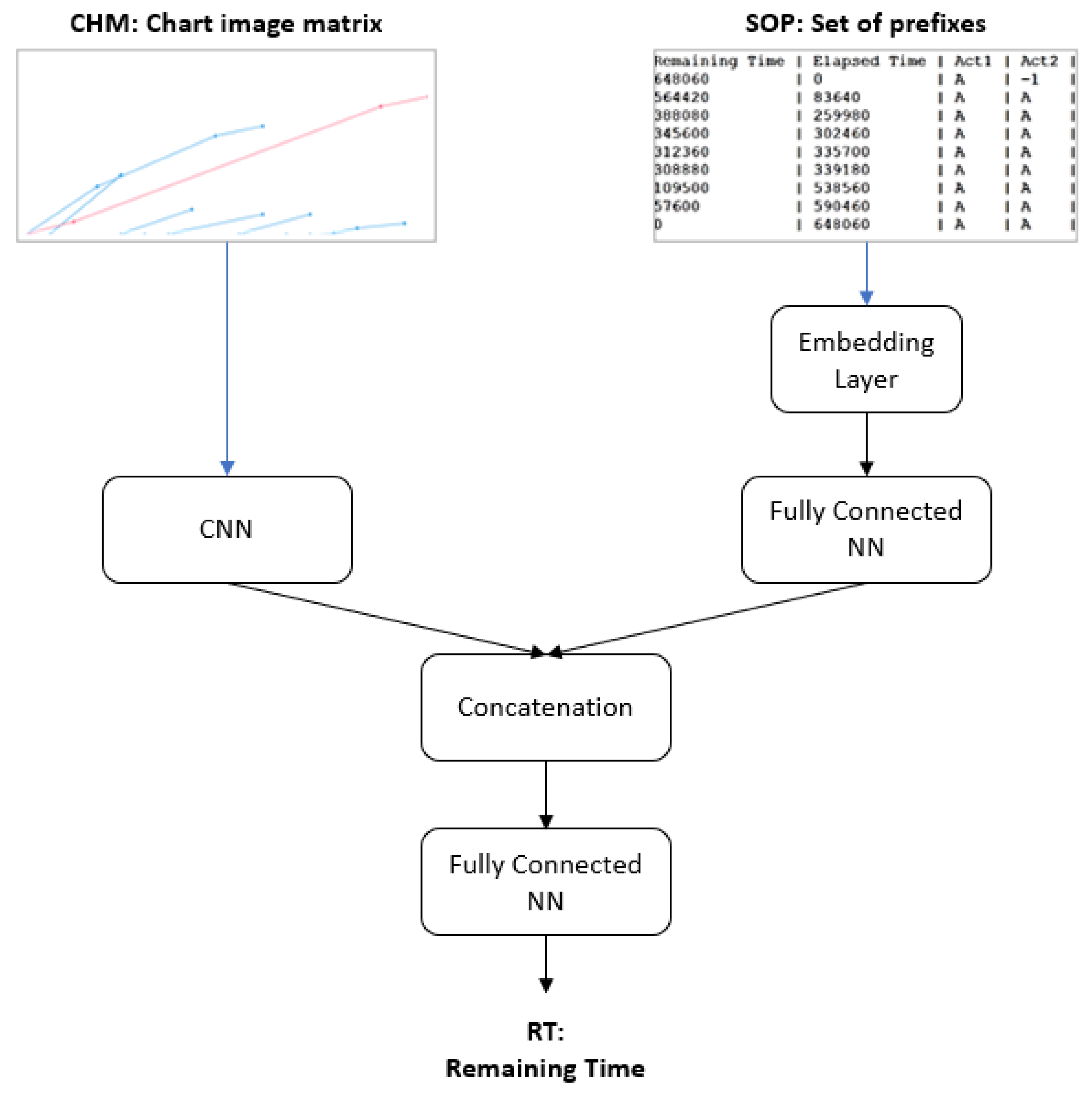
- Development of an NN architecture that incorporates two models, a convolutional neural network (CNN) and a multi-layer perceptron with data-aware entity embedding (MLP + DAEE), and the proposal of a new method of encoding as applied to event-log-type data;
- Improvement of the accuracy of a deep-learning-based method for the prediction of the remaining time of an ongoing case problem, as confirmed by comparing our method with another deep-learning method used as a baseline method;
- Experimental demonstration that the utilization of chart image representation, specifically the inter-case dependency feature contained therein, can increase the accuracy over the remaining time of the ongoing process prediction problem;
- Provision, to PBPM, of a functional solution in the form of an introduced new deep-learning-based method that does not use a recurrent NN. (To date, all deep-learning-based methods use a recurrent NN.)
1.2. Definitions and Problem Statement
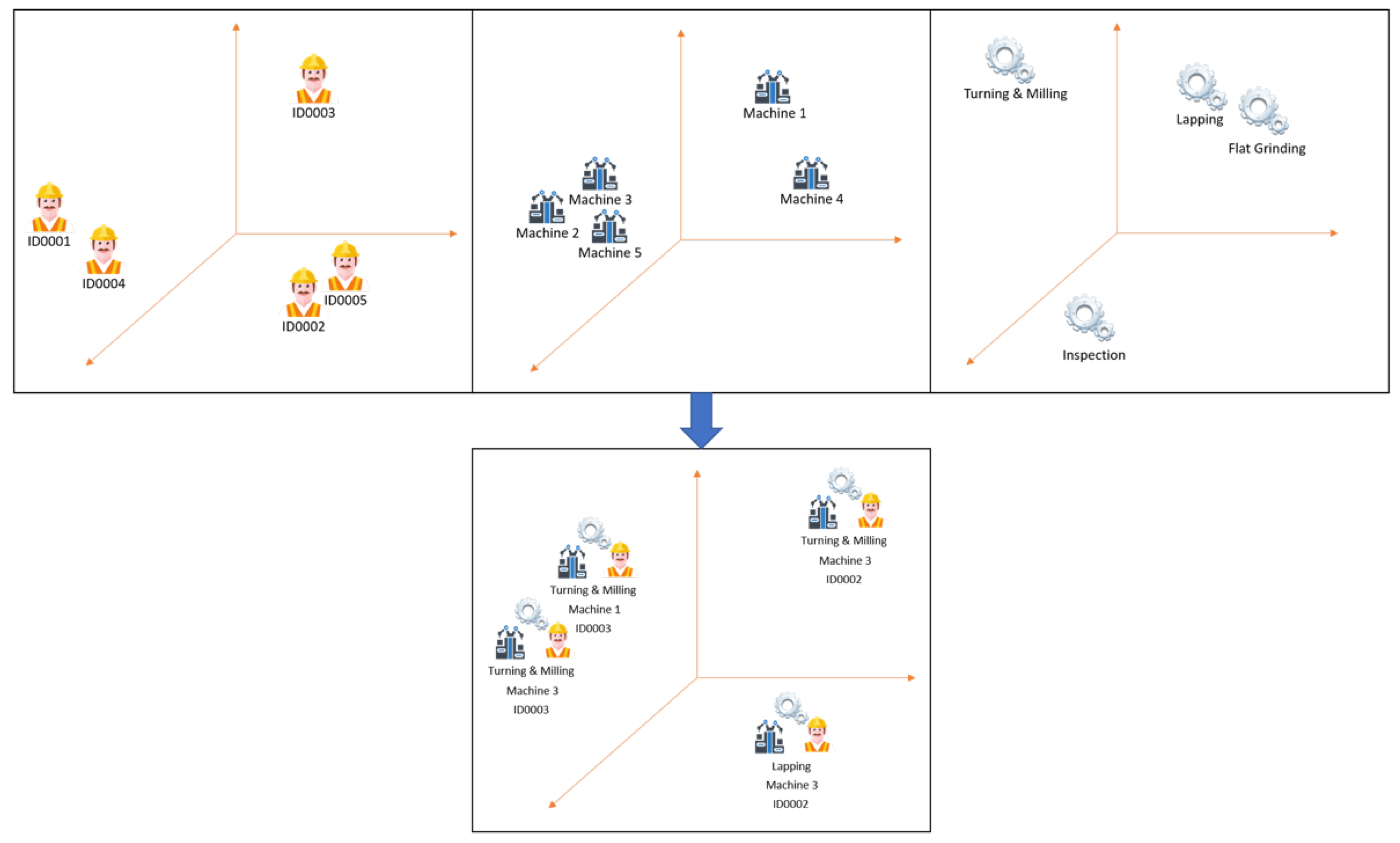
- Definition 2.1.1 (Event). An event is a tuple denoted where is the activity of the process associated with the event, , while is a finite set of process activities, is the case identifier, , is a set of all case identifiers, is the timestamp of the event, , is the time domain, is a list of other attributes of the event, , and is a set of all possible values of attribute- . The event universe is denoted . At each event we also define the mapping functions: , , , where , .
- Definition 2.1.2 (Case). A case is a finite sequence of events denoted , where is the set of all possible sequences over , , , and is the event in case at index . An ongoing case is a prefix case of length , denoted .
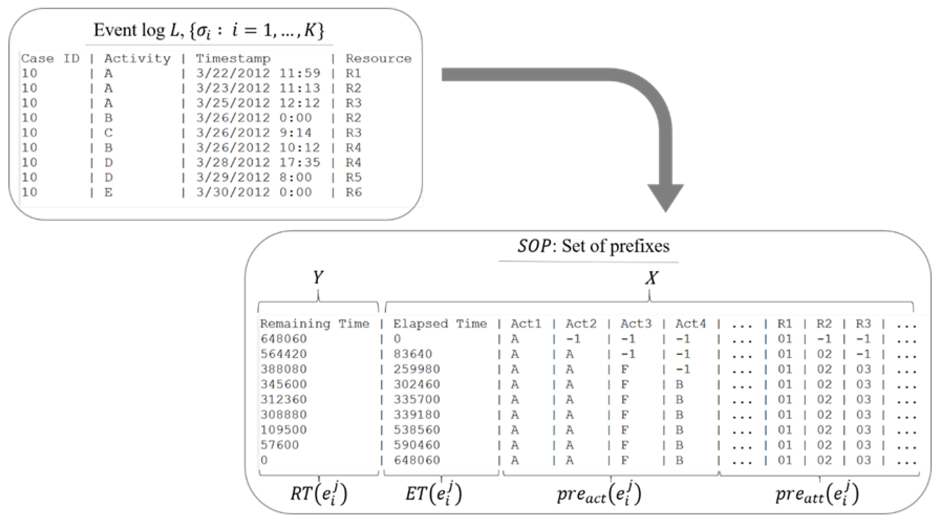
- Definition 2.1.3 (Event log). An event log is a set of -sized cases, denoted such that each event appears at most once in the event log. So, we can write the th case of length as .
- Definition 2.1.4 (Set of prefixes). A set of prefixes is a converted event log of -size, where , which contains the prefixes and other essential properties of all events as tuples, denoted , with , where is the remaining time of a prefix case, , is the elapsed time of a prefix case, , is the tuple of a prefix of activities, i.e., , is the tuple of a prefix of attributes, i.e., , is the timestamp of the last event in the prefix case, while is the case identifier of the prefix case, , . We also define the mapping functions and that return and respectively at the th .
2. Related Work
3. Proposed Method
3.1. Framework
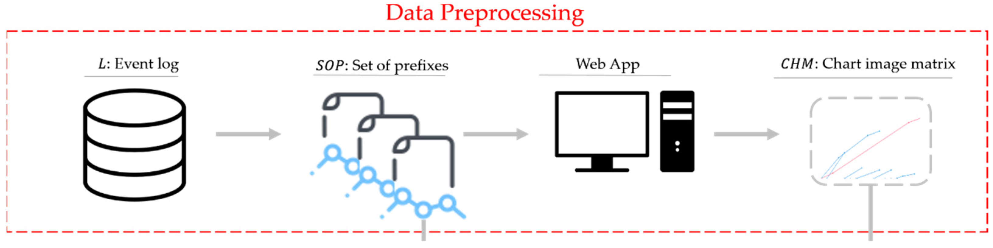
3.2. Data Preprocessing
3.2.1. Event Logs to Set of Prefixes (SOP)
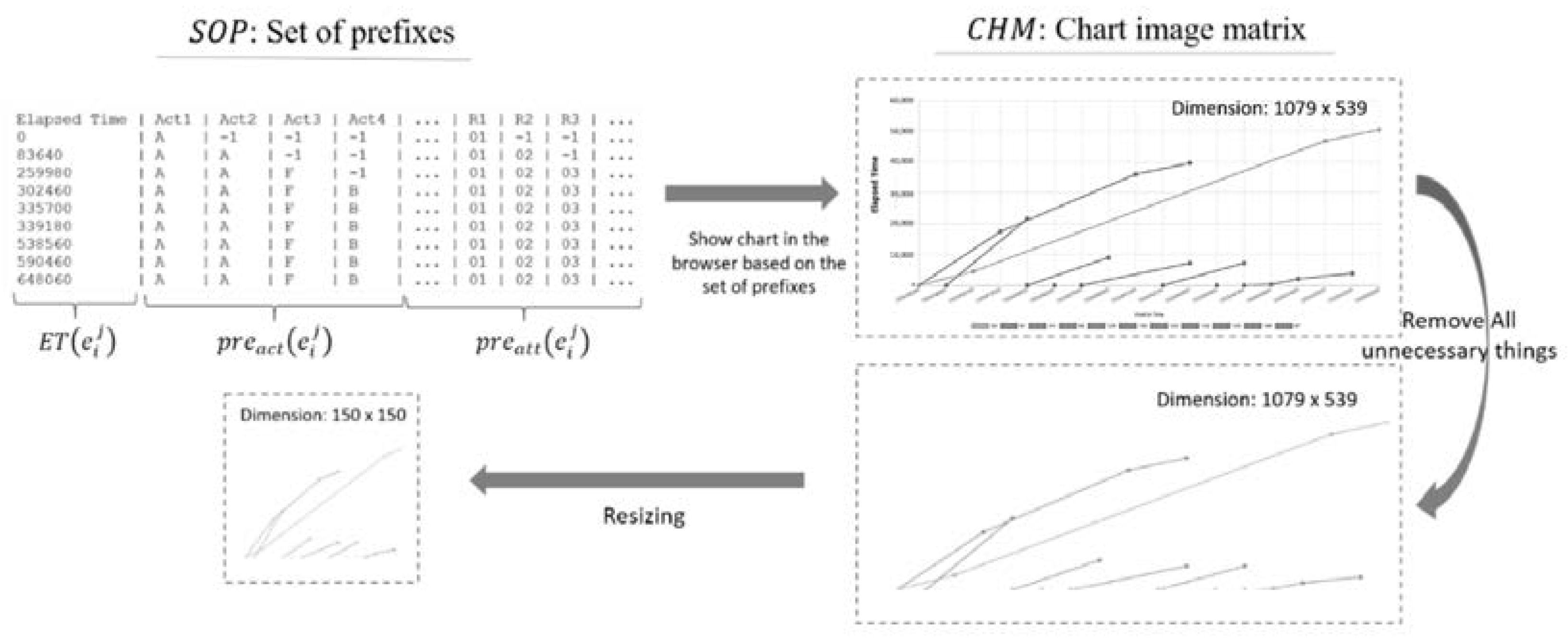
3.2.2. Convert the Set of Prefixes (SOP) to Chart Image
3.3. Network Architecture
3.3.1. Multi-Layer Perceptron with a Data-Aware Entity-Embedding Layer
| Algorithm 1. DAEE Build-Up from SOP |
| Input: : Event log, , : Set of prefixes, , sorted by its Output: : Data-Aware Events Begin 1: 2: 3: for do 4: 5: for do 6: 7: 8: for do 9: 10: end for 11: 12: end for 13: 25: return End |
3.3.2. Convolutional Neural Network (CNN)
3.3.3. DAEE and CNN Output Concatenation
4. Experimentation and Results
4.1. Data Description
4.2. Experimental Setup
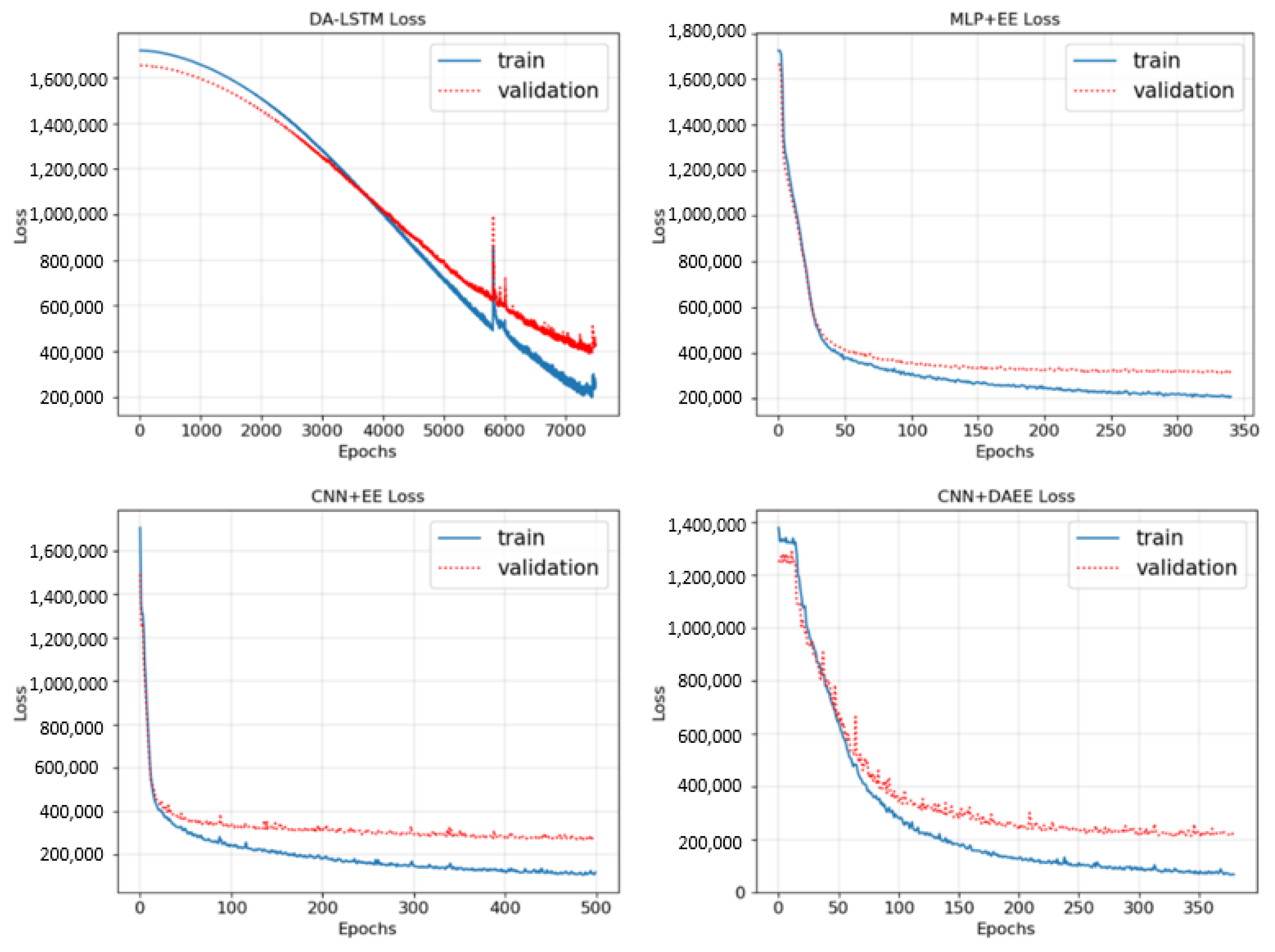
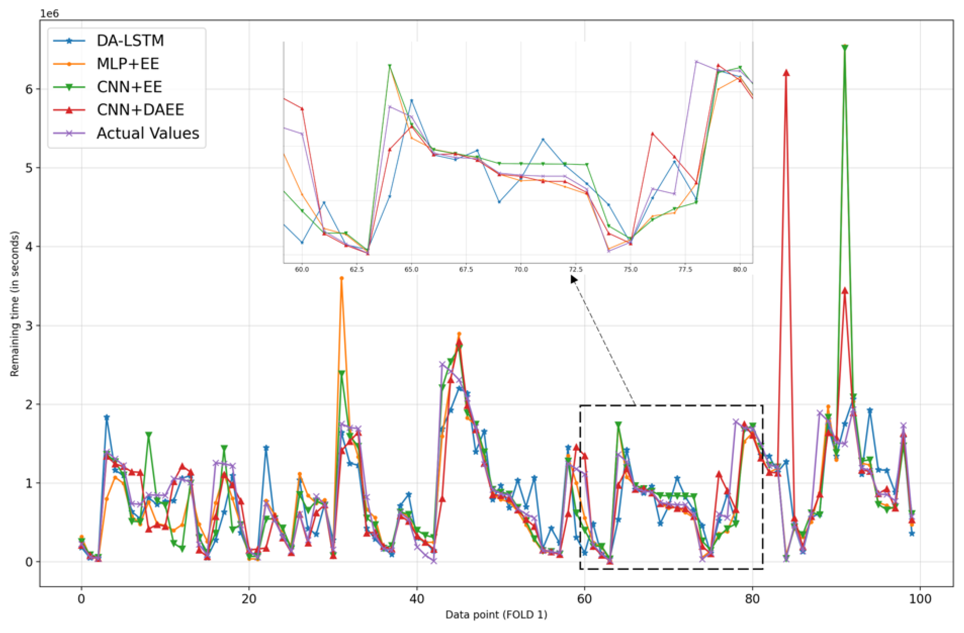
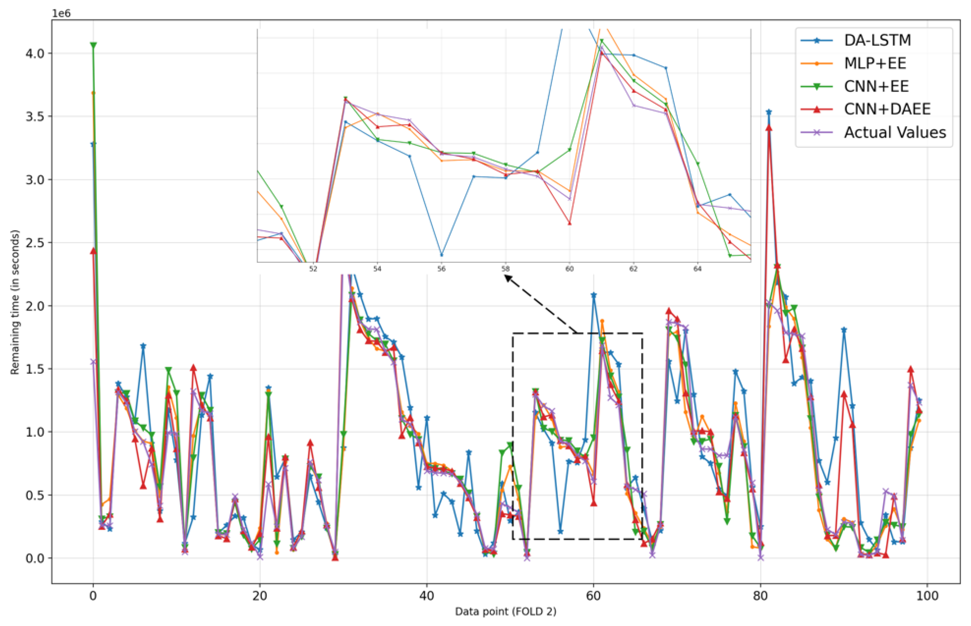
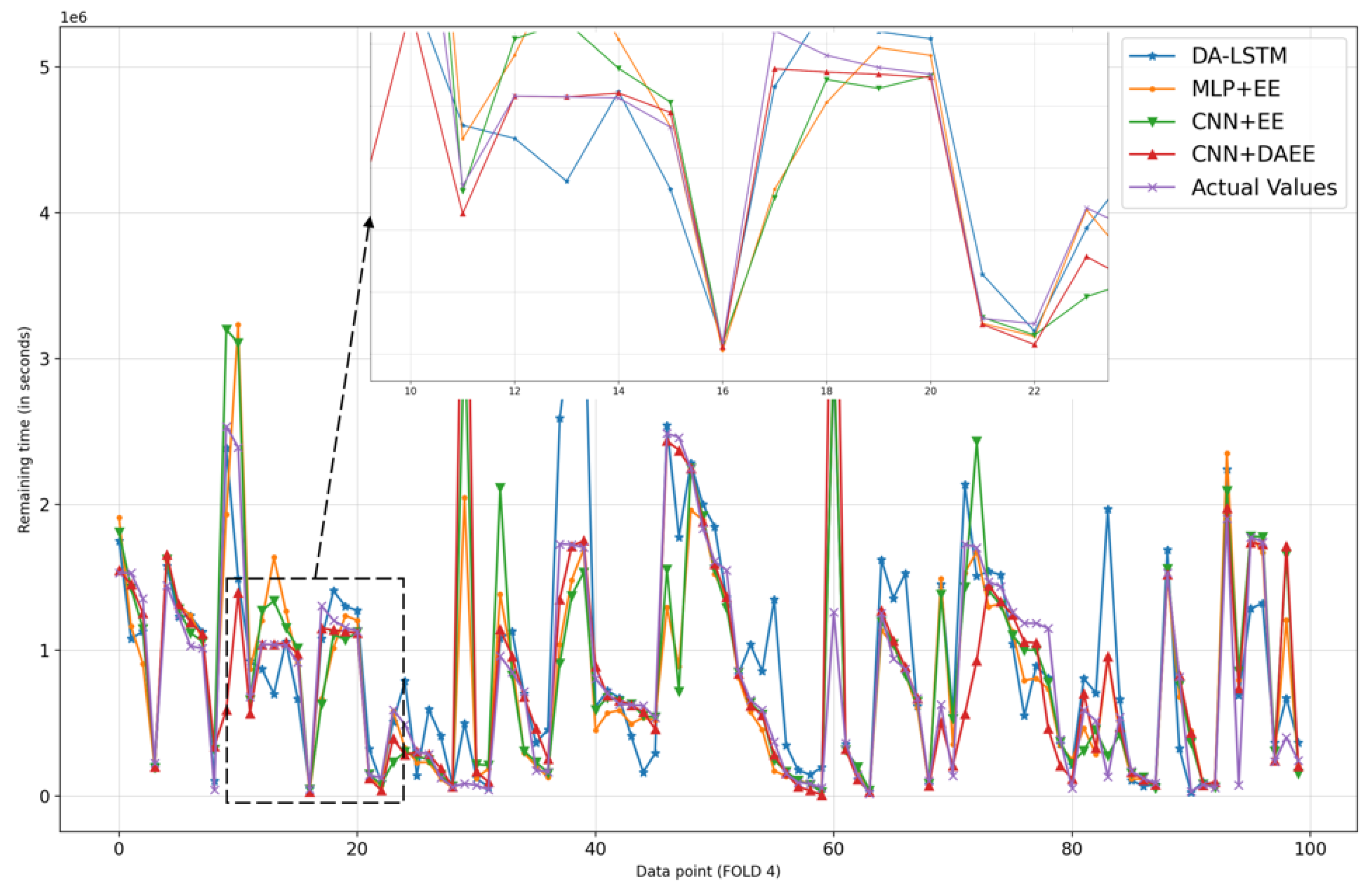
- CNN + DAEE, our full proposed method, consists of a combination of two NN models, CNN and MLP with DAEE;
- CNN + EE, the same model as CNN + DAEE, except that it uses entity embedding as its encoder;
- MLP + EE, which is one part of our proposed method without the CNN model, to show the impact of not utilizing chart images;
- DA-LSTM, the latest method based on deep learning for the prediction of the remaining time of an ongoing process problem.
4.3. Results
5. Discussion and Conclusions
Author Contributions
Funding
Acknowledgments
Conflicts of Interest
References
- Van der Aalst, W. Process Mining; Springer: Berlin/Heidelberg, Germany, 2016; ISBN 978-3-662-49850-7. [Google Scholar] [CrossRef]
- Maggi, F.M.; Francescomarino, C.D.; Dumas, M.; Ghidini, C. Predictive Monitoring of Business Processes. In Advanced Information Systems Engineering; Springer International Publishing: Berlin/Heidelberg, Germany, 2014; pp. 457–472. [Google Scholar]
- Van der Aalst, W.M.P.; Schonenberg, M.H.; Song, M. Time prediction based on process mining. Inf. Syst. 2011, 36, 450–475. [Google Scholar] [CrossRef] [Green Version]
- Schmidhuber, J. Deep learning in neural networks: An overview. Neural Netw. 2015, 61, 85–117. [Google Scholar] [CrossRef] [PubMed] [Green Version]
- LeCun, Y. Deep learning & convolutional networks. In Proceedings of the 2015 IEEE Hot Chips 27 Symposium (HCS), Cupertino, CA, USA, 22–25 August 2015. [Google Scholar] [CrossRef]
- Van Dongen, B.F.; Crooy, R.A.; van der Aalst, W.M.P. Cycle Time Prediction: When Will This Case Finally Be Finished? In On the Move to Meaningful Internet Systems: {OTM} 2008; Springer: Berlin/Heidelberg, Germany, 2008; pp. 319–336. [Google Scholar] [CrossRef]
- Folino, F.; Guarascio, M.; Pontieri, L. Discovering Context-Aware Models for Predicting Business Process Performances. In On the Move to Meaningful Internet Systems: {OTM} 2012; Springer: Berlin/Heidelberg, Germany, 2012; pp. 287–304. [Google Scholar] [CrossRef]
- Leontjeva, A.; Conforti, R.; Di Francescomarino, C.; Dumas, M.; Maggi, F.M. Complex Symbolic Sequence Encodings for Predictive Monitoring of Business Processes. In Lecture Notes in Computer Science; Springer International Publishing: Berlin/Heidelberg, Germany, 2015; pp. 297–313. [Google Scholar] [CrossRef] [Green Version]
- Senderovich, A.; Weidlich, M.; Gal, A.; Mandelbaum, A. Queue mining for delay prediction in multi-class service processes. Inf. Syst. 2015, 53, 278–295. [Google Scholar] [CrossRef] [Green Version]
- De Leoni, M.; van der Aalst, W.M.P.; Dees, M. A general process mining framework for correlating, predicting and clustering dynamic behavior based on event logs. Inf. Syst. 2016, 56, 235–257. [Google Scholar] [CrossRef]
- Di Francescomarino, C.; Dumas, M.; Federici, M.; Ghidini, C.; Maggi, F.M.; Rizzi, W. Predictive Business Process Monitoring Framework with Hyperparameter Optimization. In Advanced Information Systems Engineering; Springer International Publishing: Berlin/Heidelberg, Germany, 2016; pp. 361–376. [Google Scholar] [CrossRef]
- Evermann, J.; Rehse, J.-R.; Fettke, P. A Deep Learning Approach for Predicting Process Behaviour at Runtime. In Business Process Management Workshops; Springer International Publishing: Berlin/Heidelberg, Germany, 2017; pp. 327–338. [Google Scholar] [CrossRef]
- Tax, N.; Verenich, I.; La Rosa, M.; Dumas, M. Predictive Business Process Monitoring with LSTM Neural Networks. In Advanced Information Systems Engineering; Springer International Publishing: Berlin/Heidelberg, Germany, 2017; pp. 477–492. [Google Scholar] [CrossRef] [Green Version]
- Bai, Y.; Jin, X.; Wang, X.; Su, T.; Kong, J.; Lu, Y. Compound Autoregressive Network for Prediction of Multivariate Time Series. Complexity 2019, 2019, 9107167. [Google Scholar] [CrossRef]
- Navarin, N.; Vincenzi, B.; Polato, M.; Sperduti, A. (LSTM) networks for data-aware remaining time prediction of business process instances. In Proceedings of the 2017 IEEE Symposium Series on Computational Intelligence (SSCI), Honolulu, HI, USA, 27 November–1 December 2017. [Google Scholar] [CrossRef] [Green Version]
- Senderovich, A.; Di Francescomarino, C.; Ghidini, C.; Jorbina, K.; Maggi, F.M. Intra and Inter-case Features in Predictive Process Monitoring: A Tale of Two Dimensions. In Lecture Notes in Computer Science; Springer International Publishing: Berlin/Heidelberg, Germany, 2017; pp. 306–323. [Google Scholar] [CrossRef]
- Di Francescomarino, C.; Dumas, M.; Federici, M.; Ghidini, C.; Maggi, F.M.; Rizzi, W.; Simonetto, L. Genetic algorithms for hyperparameter optimization in predictive business process monitoring. Inf. Syst. 2018, 74, 67–83. [Google Scholar] [CrossRef]
- Yao, H.; Zhang, X.; Zhou, X.; Liu, S. Parallel Structure Deep Neural Network Using CNN and RNN with an Attention Mechanism for Breast Cancer Histology Image Classification. Cancers 2019, 11, 1901. [Google Scholar] [CrossRef] [PubMed] [Green Version]
- Zhang, W.; Wu, P.; Peng, Y.; Liu, D. Roll Motion Prediction of Unmanned Surface Vehicle Based on Coupled CNN and LSTM. Future Internet 2019, 11, 243. [Google Scholar] [CrossRef] [Green Version]
- Zheng, Z.; Chen, Z.; Hu, F.; Zhu, J.; Tang, Q.; Liang, Y. An Automatic Diagnosis of Arrhythmias Using a Combination of CNN and LSTM Technology. Electronics 2020, 9, 121. [Google Scholar] [CrossRef] [Green Version]
- Le, T.; Vo, M.T.; Vo, B.; Hwang, E.; Rho, S.; Baik, S.W. Improving Electric Energy Consumption Prediction Using CNN and Bi-LSTM. Appl. Sci. 2019, 9, 4237. [Google Scholar] [CrossRef] [Green Version]
- Shi, Z.; Bai, Y.; Jin, X.; Wang, X.; Su, T.; Kong, J. Parallel Deep Prediction with Covariance Intersection Fusion on Non-Stationary Time Series. Knowl. Based Syst. 2021, 211, 106523. [Google Scholar] [CrossRef]
- Curley, R.; Gage, R. Django Project. Available online: https://www.djangoproject.com/ (accessed on 2 October 2021).
- Vanderkam, D. Dygraphs. Available online: https://dygraphs.com/ (accessed on 2 October 2021).
- Sim, H.S.; Kim, H.I.; Ahn, J.J. Is Deep Learning for Image Recognition Applicable to Stock Market Prediction? Complexity 2019, 2019, 1–10. [Google Scholar] [CrossRef]
- Lee, J.; Kim, R.; Koh, Y.; Kang, J. Global Stock Market Prediction Based on Stock Chart Images Using Deep Q-Network. arXiv 2019, arXiv:abs/1902.1. [Google Scholar] [CrossRef]
- Nair, V.; Hinton, G.E. Rectified Linear Units Improve Restricted Boltzmann Machines. In Proceedings of the 27th International Conference on International Conference on Machine Learning, Haifa, Israel, 21–24 June 2010; Omnipress: Madison, WI, USA, 2010; pp. 807–814. [Google Scholar]
- Srivastava, N.; Hinton, G.; Krizhevsky, A.; Sutskever, I.; Salakhutdinov, R. Dropout: A Simple Way to Prevent Neural Networks from Overfitting. J. Mach. Learn. Res. 2014, 15, 1929–1958. [Google Scholar]
- Hastie, T.; Tibshirani, R.; Friedman, J. The Elements of Statistical Learning; Springer Series in Statistics; Springer New York: New York, NY, USA, 2009; ISBN 978-0-387-84857-0. [Google Scholar] [CrossRef]
- Guo, C.; Berkhahn, F. Entity Embeddings of Categorical Variables. arXiv 2016, arXiv:1604.06737. [Google Scholar]
- Wahid, N.A.; Adi, T.N.; Bae, H.; Choi, Y. Predictive Business Process Monitoring—Remaining Time Prediction using Deep Neural Network with Entity Embedding. Procedia Comput. Sci. 2019, 161, 1080–1088. [Google Scholar] [CrossRef]
- Krizhevsky, A.; Sutskever, I.; Hinton, G.E. ImageNet classification with deep convolutional neural networks. Commun. ACM 2017, 60, 84–90. [Google Scholar] [CrossRef]
- Chollet, F. Keras Library. Available online: https://keras.io/ (accessed on 2 October 2021).
- Lawrence, S.; Giles, C.L. Overfitting and neural networks: Conjugate gradient and backpropagation. In Proceedings of the IEEE-INNS-ENNS International Joint Conference on Neural Networks. IJCNN 2000. Neural Computing: New Challenges and Perspectives for the New Millennium, Como, Italy, 27 July 2000. [Google Scholar] [CrossRef]
- Kingma, D.P.; Ba, J.L. ADAM: A Method for Stochastic Optimization. In Proceedings of the 3rd International Conference on Learning Representations (ICLR 2015), San Diego, CA, USA, 7–9 May 2015; pp. 1–15. [Google Scholar]
- Levy, D. Production Analysis with Process Mining Technology. Dataset 2014. [Google Scholar] [CrossRef]
- Stone, M. Cross-Validatory Choice and Assessment of Statistical Predictions. J. R. Stat. Soc. 1974, 36, 111–147. [Google Scholar] [CrossRef]


| Author | Method | Objective |
|---|---|---|
| van Dongen, Crooy and van der Aalst (2008) [6] | Non-parametric Regression technique | Predicting the remaining time |
| van der Aalst, Schonenberg and Song (2011) [3] | Annotated Transition Systems | Predicting the remaining time |
| Folino, Guarascio and Pontieri (2012) [7] | Predictive Clustering Tree | Predicting the remaining time |
| Maggi et al. (2014) [2] | Decision Trees | Predicting the Linear Temporal Logic rules |
| Leontjeva et al. (2015) [8] | HMM and Random Forest | Predicting the outcome |
| Senderovich et al. (2015) [9] | Queueing theory | Predicting the delays |
| Francescomarino et al. (2016) | Clustering and Hyperparameters Optimization | Predicting the Linear Temporal Logic rules |
| Evermann, Rehse and Fettke (2017) [12] | Deep learning, LSTM | Predicting the next event |
| Tax et al. (2017) [13] | Deep learning, LSTM | Predicting the remaining time, the outcome, and the next event |
| Navarin et al. (2017) [15] | Deep learning, Data-Aware LSTM | Predicting the remaining time |
| Senderovich et al. (2017) [16] | Feature Engineering | Predicting the remaining time |
| Francescomarino et al. (2018) [11] | Genetic Algorithm | Optimizing the hyperparameters |
| Layer (Type) | Input Shape | Output Shape | Connected to |
|---|---|---|---|
| embed (Embedding) | (, 50) | ( 50) | input_dis_1 |
| input_dis_2 | |||
| input_dis_3 | |||
| … | |||
| input_dis_n | |||
| dense_1 (Dense) | (1) | (1) | input_cont_1 |
| dense_2 (Dense) | (1) | (1) | input_cont_2 |
| dense_3 (Dense) | (1) | (1) | input_cont_3 |
| … | … | … | … |
| dense_m (Dense) | (1) | (1) | input_cont_m |
| reshape (Reshape) | ( 50) | ( 50) | embed[1] |
| embed[2] | |||
| embed[3] | |||
| … | |||
| embed[n] |
| Layer (Type) | Input Shape | Output Shape | Connected to |
|---|---|---|---|
| concatenate_1 (Concatenate) | (1), (1), (1), … (1) ( 50), ( 50), ( 50), … ( 50) | (m (n 50)), | dense_1 dense_2 dense_3 … dense_m reshape[1] reshape[2] reshape[3] … reshape[n] |
| dense_NN_1 | (m (n 50)) | (500) | concatenate_1 |
| activation_1 (Activation) | (500) | (500) | dense_NN_1 |
| dropout_1 (Dropout) | (500) | (500) | activation_1 |
| dense_NN_2 (Dense) | (500) | (250) | dropout_1 |
| activation_2 (Activation) | (250) | (250) | dense_NN_2 |
| dropout_2 (Dropout) | (250) | (250) | activation_2 |
| dense_NN_3 (Dense) | (250) | (100) | dropout_2 |
| activation_3 (Activation) | (100) | (100) | dense_NN_3 |
| dropout_3 (Dropout) | (100) | (100) | activation_3 |
| dense_NN_4 (Dense) | (100) | (50) | dropout_3 |
| Layer (Type) | Input Shape | Output Shape | Connected to |
|---|---|---|---|
| input_image (InputLayer) | (150, 150, 3) | (150, 150, 3) | |
| conv2d_1 (Conv2D) | (150, 150, 3) | (150, 150, 32) | input_image |
| max_pooling2d_1 (MaxPooling2D) | (150, 150, 32) | (75, 75, 32) | conv2d_1 |
| conv2d_2 (Conv2D) | (75, 75, 32) | (75, 75, 64) | max_pooling2d_1 |
| max_pooling2d_2 (MaxPooling2D) | (75, 75, 64) | (37, 37, 64) | conv2d_2 |
| conv2d_3 (Conv2D) | (37, 37, 64) | (37, 37, 96) | max_pooling2d_2 |
| max_pooling2d_3 | (37, 37, 96) | (18, 18, 96) | conv2d_3 |
| conv2d_4 (Conv2D) | (18, 18, 96) | (18, 18, 96) | max_pooling2d_3 |
| max_pooling2d_4 | (18, 18, 96) | (9, 9, 96) | conv2d_4 |
| flatten_1 (Flatten) | (9, 9, 96) | (7776) | max_pooling2d_4 |
| Layer (Type) | Input Shape | Output Shape | Connected to |
|---|---|---|---|
| concatenate_2 (Concatenate) | (50) (7776) | (7826) | dense_NN_4 flatten_1 |
| dense_NN_5 (Dense) | (7826) | (512) | concatenate_2 |
| dense_NN_6 (Dense) | (512) | (100) | dense_NN_5 |
| dense_NN_7 (Dense) | (100) | (10) | dense_NN_6 |
| dense_NN_8 (Dense) | (10) | (1) | dense_NN_7 |
| Case ID | Activity | Resource | Timestamp | Work Order Qty | Part Desc. | Worker ID | Report Type | Qty Completed | Qty Rejected | Qty for MRB | Rework |
|---|---|---|---|---|---|---|---|---|---|---|---|
| Case 1 | Turning & Milling—Machine 4 | Machine 4—Turning & Milling | 1/29/12 23:24 | 10 | Cable Head | ID4932 | S | 1 | 0 | 0 | |
| Case 1 | Turning & Milling—Machine 4 | Machine 4—Turning & Milling | 1/30/12 5:44 | 10 | Cable Head | ID4932 | D | 1 | 0 | 0 | |
| Case 1 | Turning & Milling—Machine 4 | Machine 4—Turning & Milling | 1/30/12 6:59 | 10 | Cable Head | ID4167 | S | 0 | 0 | 0 | |
| Case 1 | Turning & Milling—Machine 4 | Machine 4—Turning & Milling | 1/30/12 7:21 | 10 | Cable Head | ID4167 | D | 8 | 0 | 0 | |
| Case 1 | Turning & Milling Q.C. | Quality Check 1 | 1/31/12 13:20 | 10 | Cable Head | ID4163 | D | 9 | 1 | 0 | |
| Case 1 | Laser Marking—Machine 7 | Machine 7—Laser Marking | 2/1/12 8:18 | 10 | Cable Head | ID0998 | D | 9 | 0 | 0 | |
| Case 1 | Lapping—Machine 1 | Machine 1—Lapping | 2/14/12 0:00 | 10 | Cable Head | ID4882 | D | 0 | 0 | 0 | |
| Case 1 | Lapping—Machine 1 | Machine 1—Lapping | 2/14/12 0:00 | 10 | Cable Head | ID4882 | D | 0 | 0 | 0 | |
| Case 1 | Lapping—Machine 1 | Machine 1—Lapping | 2/14/12 9:05 | 10 | Cable Head | ID4882 | D | 1 | 0 | 0 | |
| Case 1 | Lapping—Machine 1 | Machine 1—Lapping | 2/14/12 9:05 | 10 | Cable Head | ID4882 | D | 8 | 0 | 0 | |
| Case 1 | Round Grinding—Machine 3 | Machine 3—Round Grinding | 2/14/12 9:13 | 10 | Cable Head | ID4445 | S | 0 | 0 | 0 | |
| Case 1 | Round Grinding—Machine 3 | Machine 3—Round Grinding | 2/14/12 13:37 | 10 | Cable Head | ID4445 | D | 9 | 0 | 0 | |
| Case 1 | Final Inspection Q.C. | Quality Check 1 | 2/16/12 6:59 | 10 | Cable Head | ID4493 | D | 0 | 0 | 0 |
| Component | Specification |
|---|---|
| CPU | Inter(R) Core (TM) i7-7700HQ CPU @ 2.80GHz 2.81 GHz |
| GPU | NVIDIA GeForce GTX 1050—4.0 GB Dedicated GPU Memory |
| Memory | 16 GB |
| Operating System | Windows 10 |
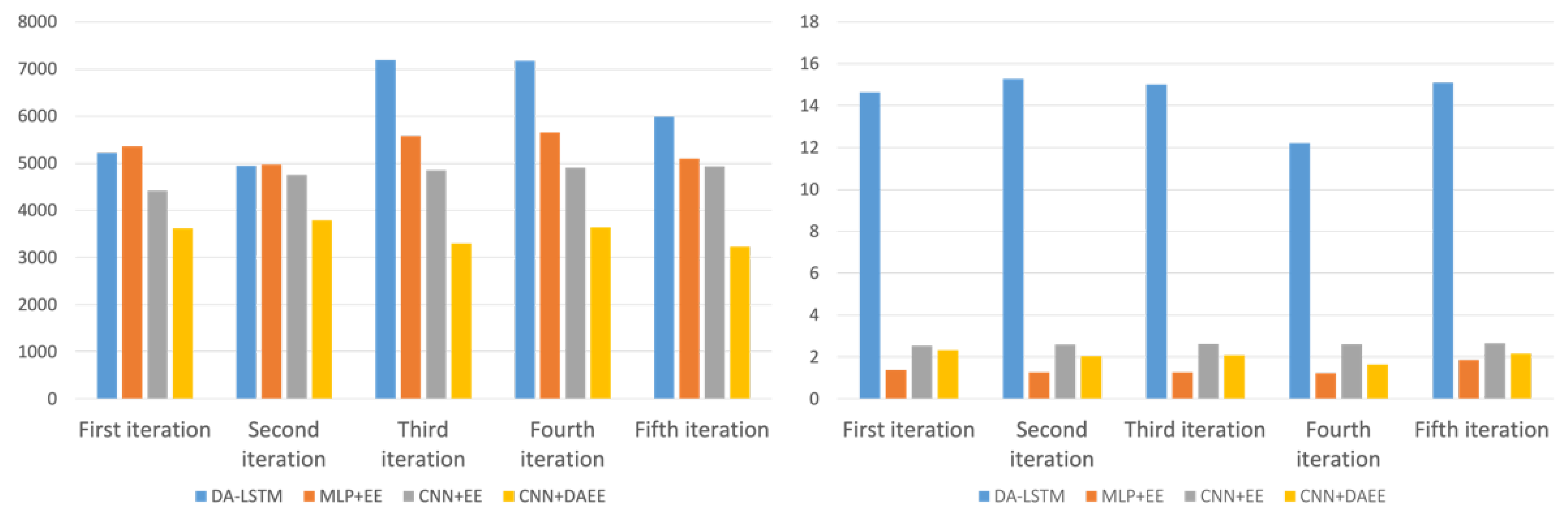
| Iteration | MAE (Minutes) | |||
|---|---|---|---|---|
| DA-LSTM | MLP + EE | CNN + EE | CNN + DAEE | |
| 1st | 5221.646 | 5362.156 | 4416.111 | 3617.575 |
| 2nd | 4945.532 | 4973.759 | 4749.251 | 3793.084 |
| 3rd | 7191.880 | 5578.992 | 4853.482 | 3301.337 |
| 4th | 7176.215 | 5654.634 | 4910.471 | 3641.002 |
| 5th | 5988.119 | 5096.931 | 4935.983 | 3232.011 |
| Iteration | Training Duration (Minutes) | |||
|---|---|---|---|---|
| DA-LSTM | MLP + EE | CNN + EE | CNN + DAEE | |
| 1st | 14:38 | 01:22 | 02:31 | 02:19 |
| 2nd | 15:16 | 01:16 | 02:35 | 02:03 |
| 3rd | 15:00 | 01:16 | 02:36 | 02:05 |
| 4th | 12:12 | 01:13 | 02:36 | 01:39 |
| 5th | 15:01 | 01:50 | 02:39 | 02:09 |
| DA-LSTM | MLP + EE | CNN + EE | CNN + DAEE | |
|---|---|---|---|---|
| MAE | 6104.678 | 5333.294 | 4773.060 | 3517.002 |
| Training duration | 861.400 | 83.600 | 155.400 | 123.000 |
Publisher’s Note: MDPI stays neutral with regard to jurisdictional claims in published maps and institutional affiliations. |
© 2021 by the authors. Licensee MDPI, Basel, Switzerland. This article is an open access article distributed under the terms and conditions of the Creative Commons Attribution (CC BY) license (https://creativecommons.org/licenses/by/4.0/).
Share and Cite
Wahid, N.A.; Bae, H.; Adi, T.N.; Choi, Y.; Iskandar, Y.A. Parallel-Structure Deep Learning for Prediction of Remaining Time of Process Instances. Appl. Sci. 2021, 11, 9848. https://doi.org/10.3390/app11219848
Wahid NA, Bae H, Adi TN, Choi Y, Iskandar YA. Parallel-Structure Deep Learning for Prediction of Remaining Time of Process Instances. Applied Sciences. 2021; 11(21):9848. https://doi.org/10.3390/app11219848
Chicago/Turabian StyleWahid, Nur Ahmad, Hyerim Bae, Taufik Nur Adi, Yulim Choi, and Yelita Anggiane Iskandar. 2021. "Parallel-Structure Deep Learning for Prediction of Remaining Time of Process Instances" Applied Sciences 11, no. 21: 9848. https://doi.org/10.3390/app11219848
APA StyleWahid, N. A., Bae, H., Adi, T. N., Choi, Y., & Iskandar, Y. A. (2021). Parallel-Structure Deep Learning for Prediction of Remaining Time of Process Instances. Applied Sciences, 11(21), 9848. https://doi.org/10.3390/app11219848