Traffic Signal Time Optimization Based on Deep Q-Network

Abstract

Because cities worldwide have high population concentration, traffic congestion is a key problem that needs to be addressed. As modern technology advances, smart traffic management is able to collect data from the environment and uses a contextual signal assignment to determine the traffic flow at intersections and improve the traffic conditions. In this paper, we propose a green signal time allocation system based on a deep Q-network (DQN) that can maximize the capacity at intersections and assign the green light time according to the traffic conditions. The proposed system also aims to reduce the standard deviation of each lane at an intersection by considering the standard deviation of the waiting time. As a result, selfish green signal allocations can be reduced. Thus, the proposed system can achieve better experimental results in a dynamic environment than those of the green signal phase sequence allocation system.

1. Introduction

Traffic congestion is worsening in cities around the world as the number of vehicles continues to increase. Traffic congestion delays the movement of vehicles and has a variety of negative consequences, such as increased travel time, waste of fuel, and increased emissions. To address the traffic congestion problem, transportation planners have proposed various transportation-related policies, including a systematic public transportation system or an alternative no-driving system. With the passing of time, the problem of traffic congestion has rapidly worsened. Therefore, there is a need for research on smart traffic signal control (TSC) that directly controls traffic flow.

Smart traffic management is an important part of transportation planning in smart cities [1]. Owing to the development of technologies such as the Internet of Things, cloud, and big data, the infrastructure of smart cities has been equipped with the latest technologies. Smart transportation management is a platform that can improve the quality of life, and its requirements are growing. Smart TSC is one of the most effective methods for efficiently reducing traffic congestion at intersections. The current traffic signal is a fixed traffic light that allocates time to a preset cycle. Fixed traffic lights always control the traffic flow with the same time distribution, which has the advantage of simplicity and no complexity. Therefore, fixed traffic lights are suitable for regular traffic flows. They are also suitable for intersections where there is not much traffic variation between lanes. However, traffic delays always occur because the actual traffic flow is unpredictable, and dynamism is bound to occur in various traffic flows.

Smart traffic lights aim to maximize capacity at intersections by controlling the traffic flow according to the environment. Therefore, they perform better than conventional fixed TSC in environments where the traffic deviations are large between lanes at intersections or the traffic volume changes over time are dynamic. In addition, congestion and environmental pollution can be reduced or wasted green light can be minimized [2]. A wasted green light means that, despite a green light being allocated to the lane, there are no vehicles leaving; therefore, the green light allocated is not being used efficiently. Traffic lights at intersections can be managed in two ways: by adjusting the time of the signal or by adjusting the signal phase sequence. The former minimizes a wasted green light by allocating the appropriate time for each situation, whereas the latter allows efficient traffic light control by distributing the green signal to the most needed lanes. For example, a traffic light that wants to minimize the waiting time of the vehicles determines that the lane with the longest waiting time is the lane that needs the longest green signal.

Various machine learning methods have been used to control traffic signals, such as fuzzy logic [3], neural networks [4], and computational intelligence [5,6]. However, fuzzy logic, which controls signals through rule-making, makes it difficult to generate effective rule sets when dealing with multiple intersections. Therefore, a traffic control system, that requires learning of dynamic environments while recognizing the surrounding intersections should apply reinforcement learning (RL) to determine the optimal decisions for the environment. This paper proposes an optimal TSC-based RL that adjusts the time of the signal.

The remainder of this paper is organized as follows. Related studies are given in Section 2. The system model and the proposed technique are formulated in Section 3. In Section 4, the experimental studies are presented and results are discussed. Finally, the concluding remarks are provided in Section 5.

2. Related Works

Many TSC approaches have been proposed in the field of traffic research, and there have been many attempts to implement a signal policy that depends on the traffic conditions. The characteristics of the intersections should be identified for the appropriate signal control. First, intersections are structures that affect each other. Vehicles pass through neighboring intersections and affect them. Second, the intersection is an unpredictable dynamic environment that varies over time or the day of the week. Intersections always face new environments. Therefore, it is not efficient to control traffic flow at the intersection with fixed traffic signal control. Moreover, traffic light control cannot be learned through supervised or unsupervised learning. This is because it is impossible to predict and set the answers to all situations pertaining to what actions should be taken under all situations. Because of the characteristics of an intersection, it is difficult to model the environment; therefore, most studies use RL [7,8].

TSC studies using RL are largely categorized according to whether the situation in the surrounding intersections is considered. A study of TSC at an isolated intersection that does not consider the circumstances in the surrounding intersections has the following advantage: it can determine more accurately and in greater detail how to implement a signal policy at a single intersection [9,10,11,12]. Therefore, it allows the implementation of the best policy to determine the traffic conditions at an isolated intersection. However, it is impossible to cope with events that occur in the surrounding intersections because the situation there cannot be determined. A TSC study that considers the situation in the surrounding intersections has the advantage of being able to implement policies for various situations, including those in the surrounding intersections [13,14,15,16,17,18]. However, its disadvantage is that the calculation complexity is high because there are many situations to consider, not just those in the target intersection but also in the surrounding intersections.

Reinforcement learning implements a policy by obtaining the information about the current traffic conditions in an intersection as a state and maximizing the rewards through interactions with the environment. The traffic signal performance depends on those parameters, which are considered as rewards. RL studies provide a variety of results depending on the design method, including the state, action, reward, and algorithms. In this paper, related studies fall into two groups: those that used the queue length and those that used the waiting time as the reward parameter.

The queue length indicates the number of vehicles waiting at the intersection. This represents the state of the intersection in the spatial domain. The waiting time indicates the average amount of time the vehicles in the intersection have waited to exit the intersection. This represents the time domain of the vehicle. In general, the queue length is considered as a reward if the aim is to minimize the number of vehicles at the intersection [9,10,13,18]. In contrast, the waiting time is considered as a reward if the aim is to minimize the waiting time of the vehicles at the intersection [11,12,14,15,16,17].

In [9], the authors proposed a deep recurrent Q-network (DQRN) technique that combines a recurrent neural network (RNN) with a deep Q-network (DQN) to learn various traffic environments. The DQRN technique builds a Q-network with long short-term memory (LSTM), which is an RNN. The objective of the DQRN is to minimize the total number of waiting vehicles before the stop line at the time unit. It has the advantage of considering not only the current state information but also a series of previous states to better distinguish the environment. In [10], the authors proposed a simple RL model that is less complex to speed up the learning. Their proposed model defines the queue length parameter in the same sense as the travel time of the vehicles. Therefore, to minimize the travel time of the vehicles, they defined the reward as the average of the queue length. In [13], the authors used a Q-value transfer strategy using a DQN to reflect the situation in the surrounding intersections. In other words, the Q-value of the surrounding intersections is reflected in the Q-value update to balance the traffic with the surrounding intersections. Therefore, the impact on the traffic conditions around the intersections can be considered. However, the approach in [13] can continuously distribute green signals to the same lane in the signal distribution. There is a concern regarding a selfish signal distribution, which assigns green signals to only one lane where there are many vehicles. In [18], the authors proposed a traffic signal timing plan that allocates the length of time. The goal is to minimize the queue length at the intersection and optimize the traffic flow. In addition, allocation of excessive green time is penalized. The experiment in [18] was conducted at multi-intersections. Because information on surrounding intersections is shared only through global optimization, the impact on learning is a concern.

In [11], the authors proposed an RL model with the goal of minimizing the total travel time. Using a transfer network, the RL model speeds up the learning through the transfer of the accumulated knowledge and it can also be learned with less data. However, only a straight green light is possible at the intersection. In other words, various green signals, such as the left direction or right direction, are not considered. In addition, only a single-intersection environment is considered. In [12], the authors minimized the aggregation of the total time spent in the queue of all vehicles using transfer RL. In [12], the Markov decision process (MDP) considers an isolated four-way intersection; therefore, if the intersection structure changes, the MDP must be modified accordingly. In addition, in [14], the authors proposed an RL model using neural fitted Q-iteration (NFQI). The aim of this NFQI-based RL model is to minimize the waiting time. The traffic environment changes dynamically over time. However, it does not reflect the traffic conditions on the time-domain flow. In [15], the authors proposed signal control in a multi-intersection environment to reduce the travel times. It selects which lanes get a green light. It can be extended from a single- to a multi-agent DQN through transfer learning. In [16], the authors proposed a method for controlling the flow of vehicles by changing the timing of the green and red traffic lights using RL. The goal is to minimize the average waiting time of the vehicles. It considers the surrounding intersections by giving their Q-value to the intersection agent next to the intersection agent directly sending the vehicles to their intersection. In this way, the intersection identifies the surrounding situation and controls the traffic flow. A limitation of the method in [16] is that the signal is simple: only green and red lights can be controlled. In [17], the authors proposed a TSC technique that allocates green signals to the lane that needs them to reduce the total travel time. In addition, because the length of the green time can be adjusted as necessary, customized signal control according to the situation is possible. However, it can be very complex depending on the number of signal orders. Accordingly, high complexity is a concern.

Other studies have described the states of intersections using 2N-dimensional feature vectors [11,12,14]. An intersection is represented as a 2N-dimensional feature vector; if a vector element has a vehicle in that position, its value is set to 1; otherwise, it is set to 0. In [11,12], studies that consider a single intersection are discussed; however, there are differences in what the 2N-dimensional vector represents. In addition, in [11], the vector reflects only the position and speed of the vehicles, whereas in [12] it contains additional information regarding the current light configuration. By contrast, the approach in [14] considers the surrounding intersections and includes information about the lane where the vehicle exits the intersection in the vector. The use of a 2N-dimensional feature vector has the advantage of accurately representing the current environment. However, it can increase the complexity of the data as the structure of the intersection changes.

In the present paper, a TSC technique is proposed that considers the situation of the surrounding intersections. The proposed technique adjusts the signal time to maximize the capacity and minimize wasted green light time. In addition, it aims to prevent selfish signal distribution by setting the order of signal assignment. Moreover, a new technique is proposed that does not modify the MDP even if the intersection structure has changed.

3. Problem Formulation

The multi-intersection TSC optimization problem involves maximizing the capacity of the target intersection through cooperation with the surrounding intersections. Capacity is defined as the number of vehicles passing through an intersection during a unit of time. The waiting time denotes the amount of time it takes a vehicle to exit the intersection from the time it stops at the intersection. A large capacity at the intersection results in fewer waiting vehicles at the intersection and shorter waiting times for them.

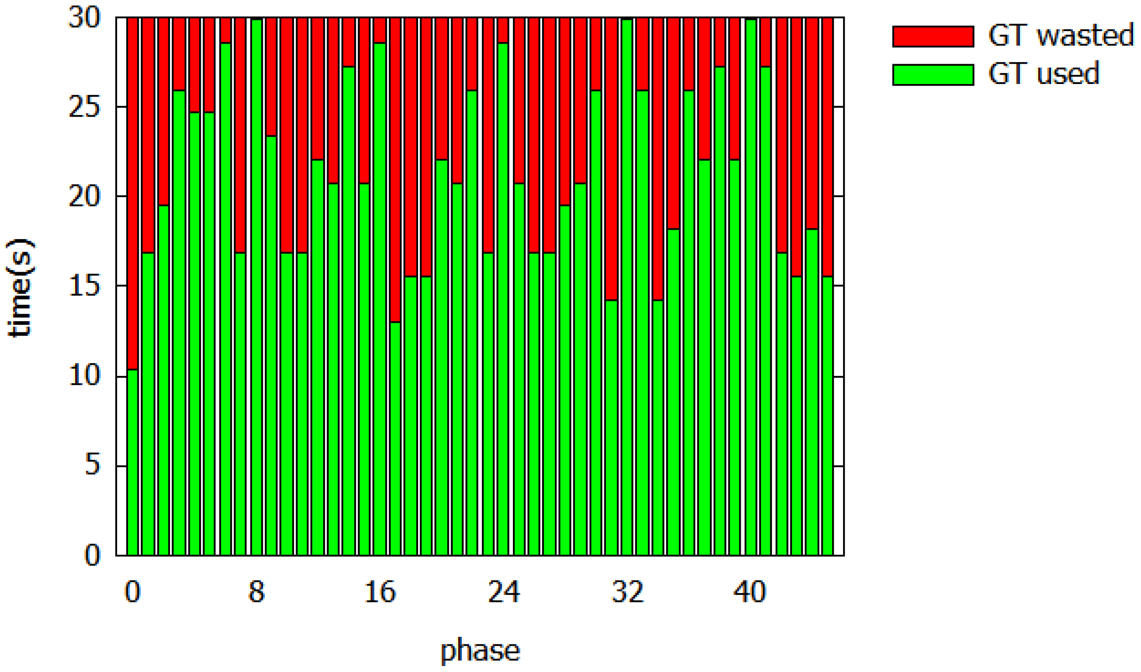
To increase the capacity at an intersection, it is important to optimize traffic signals. Specifically, the efficiency of green signals is important for handling many vehicles at an intersection. The more vehicles exit during a given green signal, the greater is the capacity at the intersection during the time unit. However, a fixed traffic signaling can cause green signal wastage because the green signal times are constant regardless of the traffic conditions. Green signal wastage means that although the lane has been allocated green light, there are no vehicles waiting; thus, there are no vehicles leaving the lane. Minimizing the wastage of green signals improves the capacity at an intersection.

Figure 1 shows an example of the time wasted on green signals at a single intersection using a fixed TSC. This experiment was conducted to analyze the efficiency of green lights in a fixed signaling system. The intersection used in this experiment was in the form of a single intersection with a four-way structure; the impact from the surrounding intersections was not considered. The distribution of vehicles used in the experiment was based on data with low traffic load. This is because a lower traffic load can more clearly show the impact of green signal wastage. According to Weijermars and van Berkum [19], the time of day with less traffic load in urban areas is before 8 am or after 8 pm on weekdays. Therefore, we conducted the experiments using traffic data from the early hours of the day in an urban area.

The experiment result showed that approximately 30% of the green signal time was wasted in the fixed signaling system. This is because more green signal time is allocated than is needed. When the duration of green signals is distributed efficiently, more vehicles can be handled at an intersection. However, dynamic green-time assignments can cause a selfish signal distribution. Intersections are chain structures that are connected to the surrounding intersections. Consequently, there can be situations in which only high-demand lanes receive signals to handle many vehicles at an intersection. In other words, the selfish distribution of signals may result in lanes not receiving green signals. A traffic signal system should distribute signals to all lanes. Therefore, a fair and reasonable signal distribution is important.

3.1. Deep Q-Network

To solve the problem of TSC, this study uses a DQN, which is an RL method. DQN defines the environment, recognizes the current state ($s_t$) at time t, selects a possible action ($a_t$), and receives a reward ($r_t$) for the result. The value for the selected action is defined as the value ($y_t$) at time t, and the value predicted by the DQN model is defined as the predicted value ($Q_{s,a}$):

$$L_t\left({\theta }_t\right)={\mathbb{E}}_{s,a}\left[\begin{array}{c}{(y_t-Q(s,a;{\theta }_t))}^2\end{array}\right].$$

(1)

The Q-network updates the network weights ($\theta$) through neural network learning by setting the minimum value of the loss function (L) to (1). In addition, a DQN consists of neural networks that are Q-networks because DQN combines Q-learning and deep learning. Therefore, it has the advantage of proceeding with learning using high-dimensional input. However, a DQN has a disadvantage in that it collects data sequentially over time in the environment. These data are then used as the input data. Because sequential data have high correlations, experience replay is applied to solve the data correlation problems. Experience replay is a method of storing the experience obtained at each time in the environment and randomly selecting the experience to learn by organizing a mini-batch. This can reduce the high correlation between the data and increase the data reliability.

3.2. Proposed DQN-Based Traffic Signal Control

The traffic signal problem of an intersection should be addressed by considering the characteristics of the intersection, which are dynamic and unpredictable. Traffic conditions change continuously depending on the time, day of the week, or weather. Intersections constantly face new environments. Moreover, the intersection has a continuous structure. The environment is computationally complex because it is affected by the circumstances in the surrounding intersections. In RL, the environment is modeled as an MDP. An MDP is defined as a state, action, or reward.

To optimize the signal control, we need to accurately recognize the current state in the MDP. In addition, it is necessary to recognize the situation in the surrounding intersections for cooperation. The state includes six pieces of information: the first and second are the information about the total traffic load ($i_1$) and the standard deviation of the traffic load ($i_2$) at the intersection, respectively. The combination of these two parameters provides a detailed representation of the situation at the intersection. For example, if the traffic load and its standard deviation are both small, there are not many vehicles at the intersection in general. However, a small traffic load with a large standard deviation indicates that, despite few vehicles being at the intersection, there are blocked lanes. Moreover, a large traffic load means that the intersection suffers from traffic congestion regardless of the standard deviation of the load.

The third ($i_3$) and fourth ($i_4$) pieces of information denote the traffic load of the two directions that will receive the next green light. The fifth ($i_5$) and sixth ($i_6$) pieces of information are regarding the traffic load in the directions where the vehicle will exit from the two directions that will receive the next green light. The proposed model provides green signals in two directions according to a traffic signal order. 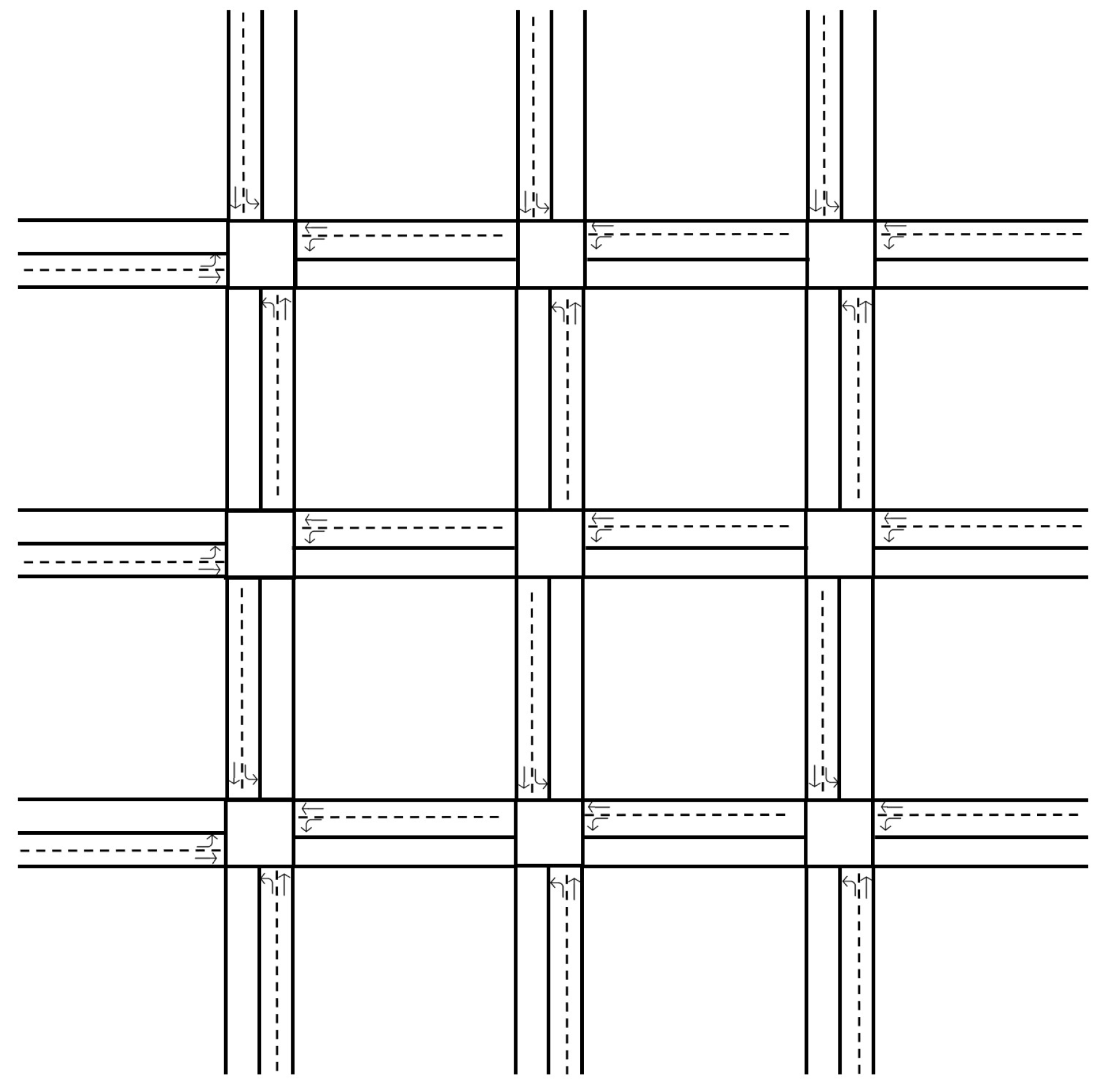Figure 2 shows the movement information when the vehicle receives a green signal. The intersection in Figure 2 is divided into two directions per road. One is the left-turn direction, and the other is the straight direction where right turns are possible. For example, if the next green signal is scheduled to be assigned the northbound straight or the right-turn direction ($l_1$) and left-turn direction ($l_2$), the vehicles waiting in $l_1$ will flow in the direction $l_3$ and the vehicles waiting in the $l_2$ direction will flow in the direction $l_4$. In this case, traffic load information in directions $l_1$ and $l_2$ is $i_3$ and $i_4$, respectively, and that in directions $l_3$ and $l_4$ is $i_5$ and $i_6$, respectively.

The information regarding the directions where the vehicle flows in when the green signal is on is needed because the number of vehicles that want to enter from a certain direction depends on the traffic load in the outgoing direction. This is because no matter how many green signals are allocated to the direction receiving the green signal, the number of vehicles that can enter is limited if there is a high traffic load in the directions that they are trying to enter. Therefore, if the time for a green signal is to be efficiently allocated, the traffic conditions in the surrounding intersections where the vehicle is about to enter should also be recognized. Therefore, the state of the MDP recognizes the current situation at the intersection with the following six pieces of information: $s_t=[i_1,i_2,i_3,i_4,i_5,i_6]$.

The proposed optimal TSC system adjusts the time of the traffic signal with the action of the MDP to efficiently use the green signal. Therefore, it is important to distribute the green signal to the required lanes at the appropriate time. An efficient green time allocation can maximize the overall capacity of the intersections. The proposed model controls the time of the green signals; moreover, it is assumed that the lane order in which the green signal is assigned is fixed, as shown in Figure 3. Therefore, the action is defined as the duration of the green signal time. We define the time unit as $\sigma$; the action of the proposed model is defined as follows: $a_t=[{\sigma }_1,{\sigma }_2,{\sigma }_3,{\sigma }_4,{\sigma }_5,{\sigma }_6,{\sigma }_7]$.

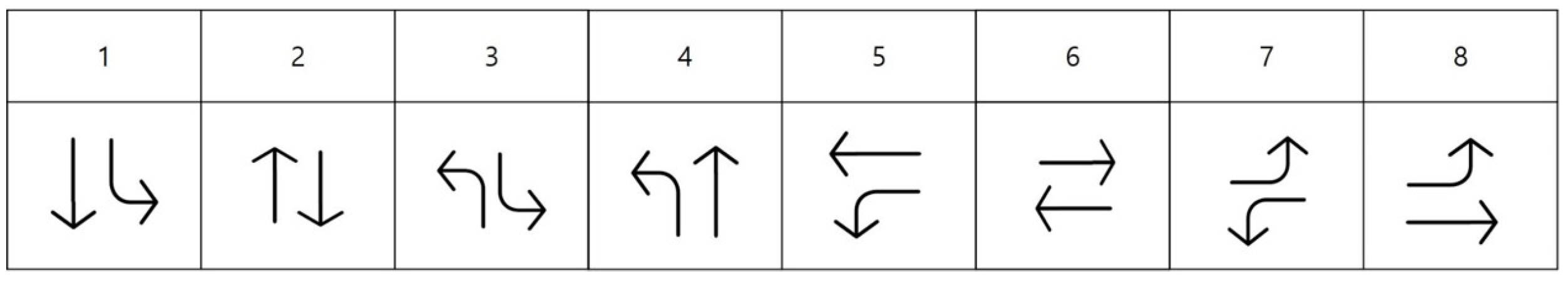
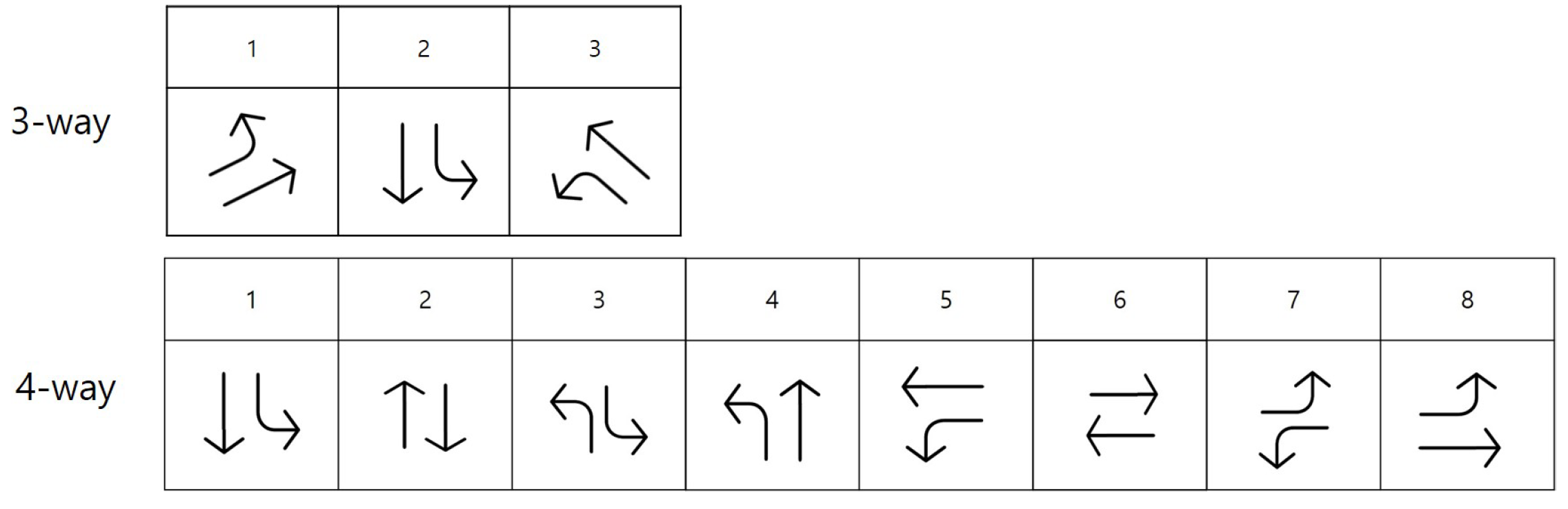
The number of lanes varies depending on the structure of the intersection; the number of lanes assigned with green lights also varies. Figure 4 shows the structure of three- to six-way intersections. As can be seen in Figure 5, there can be three possible signal directions at a three-way intersection and eight at a four-way intersection. The five- and six-way intersections have more signal directions than those of the four-way intersection. As such, the number of signal directions varies for each intersection structure. Therefore, the number of signal directions is affected by the structure of the intersection.

Time is an essential factor when allocating signals to lanes at traffic lights. Each signal direction has a certain length of time during which the vehicles exit the intersection. This length of time does not have to change even if the structure of the intersection changes. Therefore, the time duration of the signal is not affected by the structure of the intersection. Therefore, the signal control model for determining the order of the signal direction has to be changed according to the structure of the intersection. However, the model that determines how long the green light lasts in each direction does not have to change depending on the structure of the intersection. In other words, the proposed MDP does not determine the order of the progress of the vehicles according to the action; rather, it determines it according to the duration of the green signals. Thus, it is possible to apply an MDP to intersections of various structures, such as three-, four-, and five-way intersections.

The goal of this study is to maximize the capacity. In addition, for a fair and reasonable distribution of signals, all lanes have to be allocated green signals in order and the appropriate green signal time must be allocated according to traffic conditions. Therefore, the deviation in the queue length and waiting time between all lanes at the intersection can be reduced.

In this study, the waiting time, not the queue length, was considered as a reward parameter. This is because assigning waiting time as the reward parameter addresses the TSC problem by allocating an appropriate green signal time, which requires time information regarding how long vehicles must wait at an intersection. However, the queue length does not include sufficient time information on the number of vehicles waiting at the intersection. In [10], there is an expression related to waiting time and queue length as follows:

$$T=\frac{\tau \ast q}{N}+l/\mu$$

Here, T denotes the average travel time; q, the average queue length; $\tau$, the time interval; N, the number of vehicles; l, the length of the road; and $\mu$, the speed of the vehicle. In this equation, time and queue have a positive correlation. However, the concept of $\tau$ and $\mu$ related to time is applied separately from the queue length. That is, the time information includes information related to time besides information related to the queue length.

Furthermore, the standard deviation of the waiting time rather than the waiting time itself represents the information regarding the deviation between the lane where a vehicle waits for a long time and the lane where a vehicle waits for a short time at an intersection. It is therefore effective to compare the situations in each lane. In addition, if the green signal is distributed when considering only a capacity maximization, the green signal can be distributed in favor of only certain lanes, which can cause problems to other lanes. However, considering the standard deviation of the waiting time can address problems that may arise when distributing signals for maximum capacity. Therefore, the standard deviation of the waiting time between lanes should be kept small.

In addition, the standard deviation of the waiting time is considered as a parameter rather than the waiting time because of the specificity of the data used in learning. Figure 6 shows an increase or decrease between the average waiting time and the standard deviation of the waiting time over the time at an intersection. At approximately 30, 60, and 90 time units, the waiting time for a total of three times suddenly decreases. This is because the vehicle exits the intersection with the green light. The average waiting time has a large range of changes when the vehicle exits the intersection. The instantaneous value of the change is recognized as a significant value that affects the learning. Thus, the value of the standard deviation of the waiting time is more stable than the average waiting time when a sudden change occurs. In other words, sudden change can be prevented from being reflected in the learning. Therefore, we consider the standard deviation of the waiting time and the capacity as parameters to maximize the capacity at intersections with an efficient green signal distribution.

$$r_t=\alpha \ast \tau -\beta \ast w{t}_{std},$$

(2)

To maximize the performance of an intersection dealing with many vehicles, we configure the reward function with two parameters, i.e., the capacity ($\tau$) and the standard deviation of the waiting time ($w{t}_{std}$). $\alpha$ is the adaptive weighting factor, which depends on the traffic load at the intersection. It ranges between 0 and 1. $\beta$ denotes 1 – $\alpha$. The reward function is defined as (2).

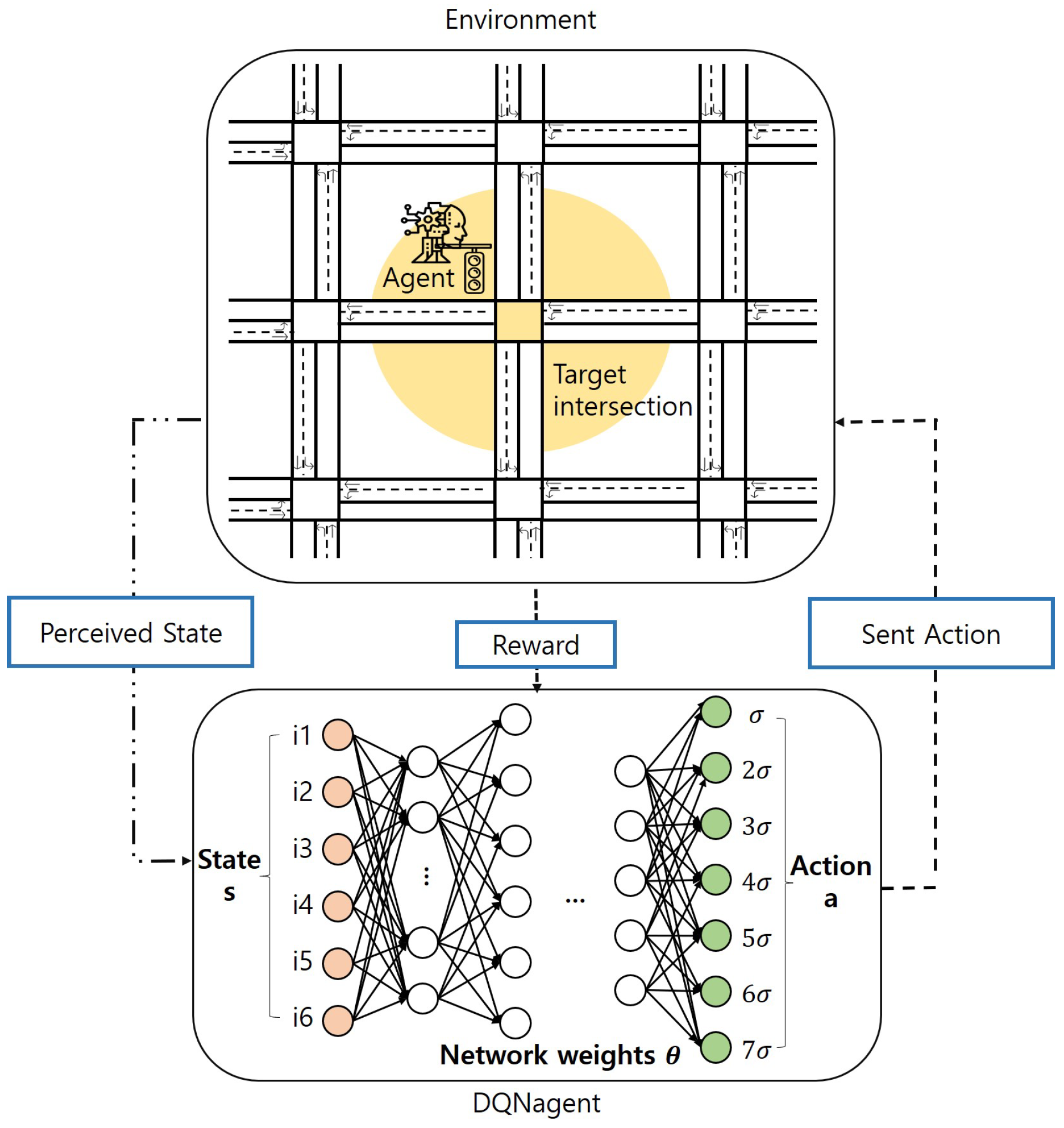
Figure 7 is a data flow chart representing the data and the process flow of the proposed model. Moreover, it shows an interaction between an environment and the agent. The environment represents several intersections. The perceived information from the target intersection, such as the waiting time of the vehicle at the intersection and the traffic load of the exit lane, is sent to the agent. Next, the agent learns from the received information and determines an action for the current state to maximize the reward. The action is sent to the environment. The action represents the time length of the green light on the lane that will move next. The performance of the traffic light control at the intersection is calculated and reflected in the learning of the agent.

4. Experimental Studies

4.1. Experimental Settings

The proposed algorithm was tested at nine successively interconnected four-way intersections, as shown in Figure 8. The average distance between intersections is approximately 200 m. The average speed of the vehicle is approximately 15 km/h and the maximum speed of the vehicle is about 50 km/h. The average speed of the vehicle was measured low because it included the speed of the vehicles waiting in the intersections. We conducted experiments to analyze the change in performance with varying the distance between the intersections and the speed of the vehicles. We extend the length of the road to from 200 m to 400 m to measure the sensitivity related to the distance and speed of vehicles. When we extend the length of the road, the average speed of vehicles was 30 km/h and the maximum speed was 70 km/h. Through experiments, we confirmed that even if the number of waiting vehicles increases due to the increase in the length of the intersection, the capacity of the intersection is similar.

The experiment was conducted using the Python API provided by the Simulation of Urban MObility (SUMO) package. SUMO is an open-source city environment and traffic flow simulator designed to handle large networks [20]. In addition, various options such as pedestrian and intersection signals can be provided to simulate the interactions with the environment, vehicles, and people. The pedestrians were not considered in this experiment. The vehicle data used in the experiment were produced in the form of a Poisson distribution using SUMO. The vehicle route data had the following settings: repetition rate of 0.5, period of 0.1, and arrival rate of 10.

In the experiments, the proposed algorithm was used with mini-batches of size 64 and a replay memory of size 3200. The learning rate of the DQN model was set to 0.001, and the discount factor was set to 0.99. The exploration rate decreased from 1 to 0.001 as the training episode continued. The model calculates the loss function using a stochastic gradient descent algorithm. The agent used k-fold cross-validation to increase the reliability of the data by using all the data for training and validation to reduce the bias of the data of the model and eliminate overfitting.

4.2. Experimental Results

The experimental results were evaluated, where the demand fluctuation follows a Poisson distribution. For the experimental results, the performance of the middle of the nine intersections was used. To test the performance of the proposed algorithm, we compared its results with those of other algorithms, namely, TFP-CTSC [21] and QT-CDQN [13]. TFP-CTSC considers the waiting time as a reward parameter, whereas QT-CDQN considers the queue length as a reward parameter. Both techniques under comparison also considered the surrounding intersections.

Figure 9 shows the rate of green signal waste of the middle of the nine intersections under the experimental environment. For the Poisson distribution, whereas TFP-CTSC and QT-CDQN wasted approximately 22% to 23% of the green signals, the proposed algorithm wasted only approximately 13% of them. The proposed algorithm wasted approximately 40% less green signal time than those of the other algorithms. This is because, although both TFP-CTSC and QT-CDQN were distributed in order of green time according to the situation, the time was fixed.

However, the proposed algorithm efficiently adjusted the green signal time to suit the situation. The performance results were the average queue length, standard deviation of the queue length, average waiting time, standard deviation of the waiting time, and capacity.

Figure 10 shows the change in the capacity of the intersection over time. As shown in the figure, the proposed algorithm handled approximately 40% more vehicles than those handled by TFP-CTSC and 30% more vehicles than those handled by QT-CDQN. The proposed algorithm handled more vehicles than those handled by the two other algorithms because it considers capacity as a reward parameter. In addition, the green signal time was efficiently used as the proposed algorithm considered the circumstances in the surrounding intersections. The efficient use of green signals also increased the capacity of the intersections.

Figure 11a shows the performance results of the vehicle waiting time according to the traffic load, and Figure 11b shows the results of the standard deviation of the waiting time. The performances of the waiting times of the TFP-CTSC and the proposed algorithm are lower than that of the QT-CDQN when the traffic load is less than 70%. This is because the TFP-CTSC considers the waiting time as a reward parameter. However, as the traffic load increases, the performance of the proposed algorithm is better than that of the two other algorithms. This is because each lane was given an appropriate green signal time, considering the standard deviation of the waiting times of the vehicles waiting at the intersection. The standard deviation of the waiting time of the proposed algorithm is approximately 35% shorter than that of TFP-CTSC and approximately 60% shorter than that of QT-CDQN. The proposed algorithm performs well with time-related values because it considers the standard deviation of the waiting time as a reward parameter. This indicates that the appropriate green time was distributed because the standard deviation of the waiting time of each lane in the intersection was considered.

Figure 12a shows the performance results for the queue length according to the traffic load, and Figure 12b shows the standard deviation of the queue length. The queue length is measured on the basis of the number of vehicles waiting at the intersection. In Figure 12a, the proposed algorithm has a queue length that is approximately 50% shorter than that of TFP-CTSC and approximately 45% shorter than that of QT-CDQN on average. Although QT-CDQN considers the queue length as a reward parameter, wasted green signal times occurred because the green time of the traffic signals was fixed.

5. Conclusions

This paper proposes a DQN-based TSC system that can learn optimal policies through a direct interaction with the environment. The smart TSC distributes the order of green signals according to the situation or sets the time of green signals in a fixed signal order. The proposed TSC system sets the time in a fixed signal order by considering the standard deviation of the waiting time and the capacity as parameters. To understand the situation at the intersection, we defined the state by considering the traffic loads at an intersection, the lane assigned the green light, and the lane used to exit. The aim of the proposed TSC system is to set the green signal duration time to maximize the capacity at intersections and minimize the standard deviation of the waiting time between lanes. Experimental results showed that the proposed technique has more capacity and better TSC performance than those of TFP-CTS and QT-CDQN. Accordingly, it showed effective improvement in TSC performance by controlling the duration time of the green signal according to the situation. The advantage of adjusting the time duration of the signal is that it is possible to increase the efficiency of the signal by reducing the wasted time of the green signal. In addition, because the time duration is set, it can be applied to different types of intersection regardless of the structure. However, this study has limitations in that it requires prior work to find the optimal order of signal directions. Because the traffic flow is different for each intersection, a study on the order of signal directions that can maximize the performance of traffic lights for each intersection is needed. Therefore, to apply the study results to an actual environment, we need to identify the traffic flow at the intersection and find an optimized sequence of signal directions that can maximize the performance of the TSC, as well as to find the optimal time length of the green light in each traffic direction.

In the future, we will explore a TSC system that can consider the pedestrians. In addition, we are planning to study TSC in terms of urban traffic control, such as grouping intersections with geographical characteristics through federated learning to form clusters.

References

1. Stevanovic, A. Adaptive Traffic Control Systems: Domestic and Foreign State of Practice; NCHRP Synthesis 403, Transportation Research Board; National Academy of Sciences: Washington, DC, USA, 2010. [Google Scholar]
2. Rahman, S.M.; Ratrout, N.T. Review of the fuzzy logic based approach in traffic signal control: Prospects in Saudi Arabia. J. Transp. Syst. Eng. Inf. Technol. 2009, 9, 58–70. [Google Scholar] [CrossRef]
3. Srinivasan, D.; Choy, M.C.; Cheu, R.L. Neural networks for real-time traffic signal control. IEEE Trans. Intell. Transp. Syst. 2006, 7, 261–272. [Google Scholar] [CrossRef] [Green Version]
4. Zhao, D.; Dai, Y.; Zhang, Z. Computational intelligence in urban traffic signal control: A survey. IEEE Trans. Syst. Man Cybern. Part C (Appl. Rev.) 2011, 42, 485–494. [Google Scholar] [CrossRef]
5. Singh, L.; Tripathi, S.; Arora, H. Time optimization for traffic signal control using genetic algorithm. Int. J. Recent Trends Eng. 2009, 2, 4. [Google Scholar]
6. Khanna, A.; Goyal, R.; Verma, M.; Joshi, D. Intelligent traffic management system for smart cities. In Proceedings of the International Conference on Futuristic Trends in Network and Communication Technologies, Solan, India, 9–10 February 2018; pp. 152–164. [Google Scholar]
7. Yau, K.L.A.; Qadir, J.; Khoo, H.L.; Ling, M.H.; Komisarczuk, P. A survey on reinforcement learning models and algorithms for traffic signal control. ACM Comput. Surv. (CSUR) 2017, 50, 1–38. [Google Scholar] [CrossRef]
8. Wei, H.; Zheng, G.; Gayah, V.; Li, Z. Recent advances in reinforcement learning for traffic signal control: A survey of models and evaluation. ACM SIGKDD Explor. Newsl. 2021, 22, 12–18. [Google Scholar] [CrossRef]
9. Zeng, J.; Hu, J.; Zhang, Y. Adaptive traffic signal control with deep recurrent Q-learning. In Proceedings of the 2018 IEEE Intelligent Vehicles Symposium (IV), Changshu, China, 26–30 June 2018; pp. 1215–1220. [Google Scholar]
10. Zheng, G.; Zang, X.; Xu, N.; Wei, H.; Yu, Z.; Gayah, V.; Xu, K.; Li, Z. Diagnosing reinforcement learning for traffic signal control. arXiv 2019, arXiv:1905.04716. [Google Scholar]
11. Xu, N.; Zheng, G.; Xu, K.; Zhu, Y.; Li, Z. Targeted Knowledge Transfer for Learning Traffic Signal Plans. In PAKDD (2); Springer: Cham, Switzerland, 2019; pp. 175–187. [Google Scholar]
12. Shabestary, S.M.A.; Abdulhai, B. Deep learning vs. discrete reinforcement learning for adaptive traffic signal control. In Proceedings of the 2018 21st International Conference on Intelligent Transportation Systems (ITSC), Maui, HI, USA, 4–7 November 2018; pp. 286–293. [Google Scholar]
13. Ge, H.; Song, Y.; Wu, C.; Ren, J.; Tan, G. Cooperative deep Q-learning with Q-value transfer for multi-intersection signal control. IEEE Access 2019, 7, 40797–40809. [Google Scholar] [CrossRef]
14. Nishi, T.; Otaki, K.; Hayakawa, K.; Yoshimura, T. Traffic signal control based on reinforcement learning with graph convolutional neural nets. In Proceedings of the 2018 21st International Conference on Intelligent Transportation Systems (ITSC), Maui, HI, USA, 4–7 November 2018; pp. 877–883. [Google Scholar]
15. Van der Pol, E.; Oliehoek, F.A. Coordinated deep reinforcement learners for traffic light control. In Proceedings of the Learning, Inference and Control of Multi-Agent Systems (at NIPS 2016), Barcelona, Spain, 9 December 2016. [Google Scholar]
16. Su, S.; Tham, C.K. SensorGrid for real-time traffic management. In Proceedings of the 2007 3rd International Conference on Intelligent Sensors, Sensor Networks and Information, Melbourne, VIC, Australia, 3–6 December 2007; IEEE: Melbourne, Australia, 2007; pp. 443–448. [Google Scholar]
17. Balaji, P.; German, X.; Srinivasan, D. Urban traffic signal control using reinforcement learning agents. IET Intell. Transp. Syst. 2010, 4, 177–188. [Google Scholar] [CrossRef]
18. Chin, Y.K.; Kow, W.Y.; Khong, W.L.; Tan, M.K.; Teo, K.T.K. Q-learning traffic signal optimization within multiple intersections traffic network. In Proceedings of the 2012 Sixth UKSim/AMSS European Symposium on Computer Modeling and Simulation, Valette, Malta, 14–16 November 2012; pp. 343–348. [Google Scholar]
19. Weijermars, W.; van Berkum, E.C. Daily flow profiles of urban traffic. WIT Trans. Built Environ. 2004, 75, 10. [Google Scholar]
20. Lopez, P.A.; Behrisch, M.; Bieker-Walz, L.; Erdmann, J.; Flötteröd, Y.P.; Hilbrich, R.; Lücken, L.; Rummel, J.; Wagner, P.; Wießner, E. Microscopic Traffic Simulation using SUMO. In Proceedings of the 21st IEEE International Conference on Intelligent Transportation Systems, Maui, HI, USA, 4–7 November 2018. [Google Scholar]
21. Kim, D.; Jeong, O. Cooperative traffic signal control with traffic flow prediction in multi-intersection. Sensors 2020, 20, 137. [Google Scholar] [CrossRef] [PubMed] [Green Version]
Figure 1. Green time (GT) wastage owing to the fixed green signal system.
Applsci 11 09850 g001
Figure 2. An example of movement information when the vehicle receives a green signal.
Applsci 11 09850 g002
Figure 3. Order of the green signal assignment.
Applsci 11 09850 g003
Figure 4. Structures of n-way intersections.
Applsci 11 09850 g004
Figure 5. Examples of the possible signals at three- and four-way intersections.
Applsci 11 09850 g005
Figure 6. Waiting time over overall time.
Applsci 11 09850 g006
Figure 7. Data flow chart of the proposed model.
Applsci 11 09850 g007
Figure 8. Structure of the environment for nine interconnected intersections.
Applsci 11 09850 g008
Figure 9. The rate of green time wasted.
Applsci 11 09850 g009
Figure 10. Change in the capacity of the intersection over time.
Applsci 11 09850 g010
Figure 11. Performance results: (a) average waiting time and (b) its standard deviation.
Applsci 11 09850 g011
Figure 12. Performance results: (a) average queue length and (b) its standard deviation.
Applsci 11 09850 g012aApplsci 11 09850 g012b
Publisher’s Note: MDPI stays neutral with regard to jurisdictional claims in published maps and institutional affiliations.