Article

Magnetically-Induced Pressure Generation in Magnetorheological Fluids under the Influence of Magnetic Fields

by
Purwadi Joko Widodo
,
Eko Prasetya Budiana
,
Ubaidillah Ubaidillah
and
Fitrian Imaduddin
*,†
Mechanical Engineering Department, Universitas Sebelas Maret, Jl. Ir Sutami No 36A, Surakarta 57126, Indonesia
*
Author to whom correspondence should be addressed.
These authors contributed equally to this work.
Appl. Sci. 2021, 11(21), 9807; https://doi.org/10.3390/app11219807
Submission received: 22 July 2021 / Revised: 5 October 2021 / Accepted: 12 October 2021 / Published: 20 October 2021
(This article belongs to the Special Issue Magneto-Rheological Fluids)

Abstract

:
This study aims to observe the magnitude of the Magnetorheological Fluids (MRFs) pressure due to the application of a magnetic field. This was accomplished by placing the MRFs in a U-shaped tube, then applying a magnetic field generated by a magnetic coil. A finite element simulation for the magnetic field was carried out to estimate the magnetic field strength generated by the coil variable to the current input given in the simulated apparatus. Changes in MRFs pressure were recorded using a data logger to better observe the fluid pressure phenomena occurring in the MRFs with respect to current input variations. The results showed that the magnetic field influences the MRFs fluid pressure proportionally. The slope is not constant as the magnetic field effect to the fluid pressure gets stronger when the current input is higher. However, there are also an adverse effect of heat generated in the coil in higher current, which results in coil performance degradation and reduces the magnetic field strength.

1. Introduction

As a smart material, Magnetorheological Fluids (MRFs) are discussed by many researchers due to their favourable characteristics for advanced actuator applications. Existing literature on MRFs include studies on the material’s synthesis and actuator design [1,2], behaviour modelling and control [3,4], and its applications [5]. As such, this long history of MRFs development has made it one of the foremost choices for advanced actuator development in automation technologies. Although MRFs are affected by changes in material viscosity when exposed to a magnetic field, these changes can be quickly controlled and are reversible by generating or negating the influence of the magnetic field which, in turn, influences the properties of the magnetorheological material [6].
MRFs change from a viscous liquid to a solid when exposed to an external magnetic field. This is due to changes in the MRFs structure wherein a dipole torque along the external magnetic field lines causes the ferromagnetic particles in the MRFs to form a chain-like structure. When the external magnetic field is removed, the MRFs returns to its original state within milliseconds as the particles disperse due to thermal motion. When the strength of the magnetic field increases, the pressure on the ferromagnetic particle chain structure increases, causing the MRFs’ viscosity to increase. In such cases, the yield stress that can be applied under steady conditions is proportional to the strength of the magnetic field applied. However, the yield strength varies according to the magnetization properties of the metal particles used in the MRFs which are a function of the concentration and properties of the metal particles [7].
In terms of MRFs operation modes, most studies have investigated the ability of MRFs to form a chain-like structure (barrier) when a magnetic field is applied and concluded that the formation of this barrier increases the shear stress of the material. They also note that changes in shear stress alter its ability to withstand external forces. Due to its ability to form a chain-like structure during operation, MRFs is utilized in several operating modes using certain control techniques. As such, MRFs can be operated in many ways depending on the requirements of an application.
Various every day devices, such as shock absorbers [8,9], brakes [10,11], clutches [12], earthquake dampers [13,14], control valves [15,16], mounts [17,18,19], thermal energy transfers [20], biomedical applications [21], precision polishing [22], and sound propagation devices [23,24], are made possible due to the properties of these smart materials. Based on the studies above, it is evident that MRFs are mostly used in energy dissipating devices and not in an active energy actuating device due to its operational modes.
For practical reasons, devices that use MRFs can be categorized into four operating modes: (1) shear-mode, (2) squeeze-mode, (3) valve-mode, and (4) gradient-pinch-mode [25]. These operating modes rely on value changes in the shear stress of the material when a magnetic field is applied [26]. Most studies conclude that microstructures similar to the formed chain increase the value of the force against the applied external force [27]. This change in force elicits a change in the shear strength of the MRFs, which increases the shear resistance of the material and its ability to withstand external forces. This feature is utilized in most applications that apply MRFs as a smart material.
On the other hand, only a few studies investigate MRFs as liquid possessing ferromagnetic properties, which could perform active actuation. Departing from the knowledge that the magnetic field induction is capable of causing the particle in MRFs to move in a specific direction, these movements hypothetically should be able to generate internal fluid pressure. It is, therefore, interesting to investigate the potential of MRFs in this respect. This study will observe the significance of these movements to cause an increase in the fluid pressure and analyze the relationship between the magnetic field and the fluid pressure. The results will be an essential finding that leads to discovering a new MRFs working mode. This study is started by designing a theoretical U-shaped tube apparatus in the Finite Element Method Magnetics (FEMM) software package. The simulation was conducted to calculate the respective magnetic field strength for each variation of the current input. The experiment was then conducted by arranging the U-shaped tube apparatus and installing the pressure transducer to measure the generated pressure of the MRFs for every time the current to the electromagnetic coil is changed.

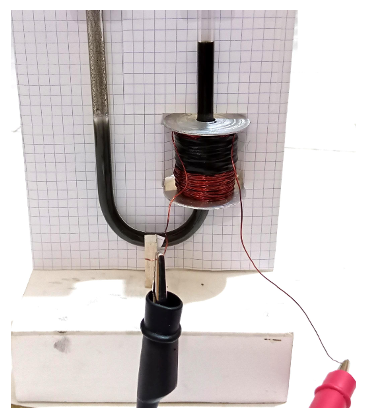
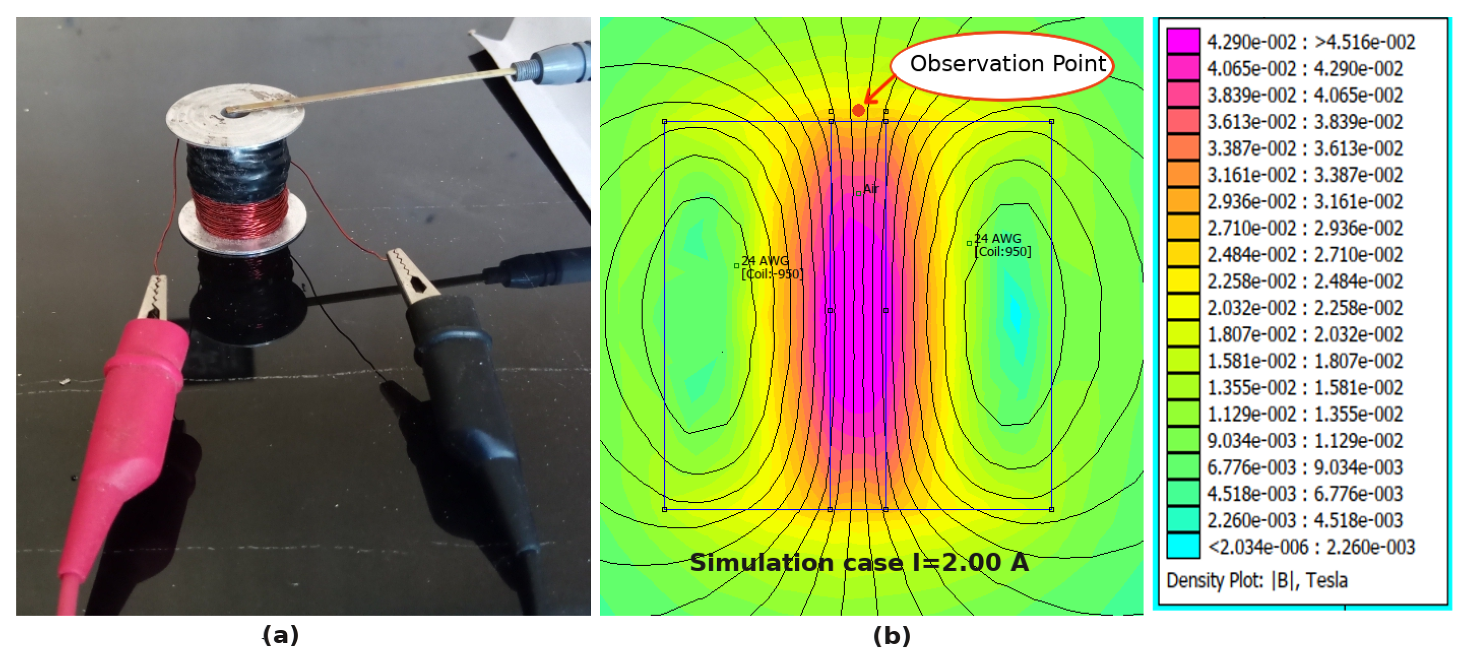
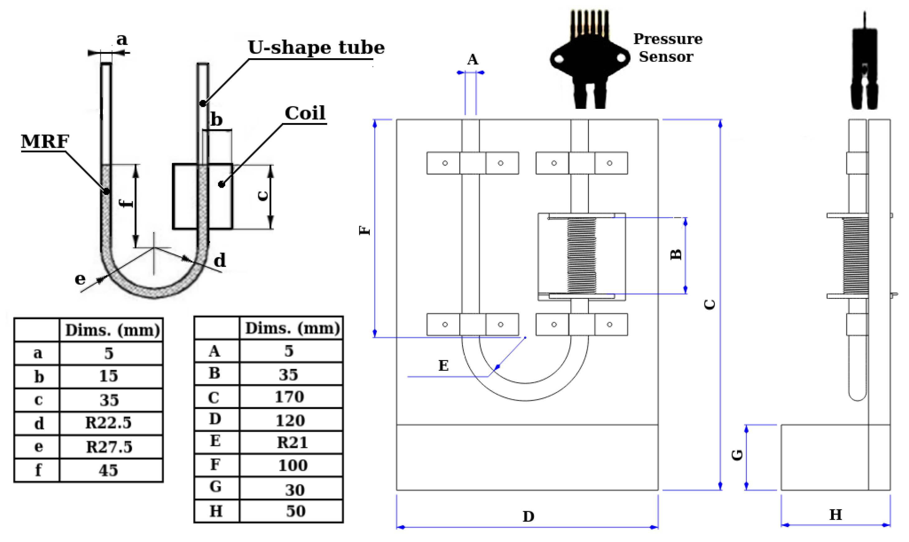
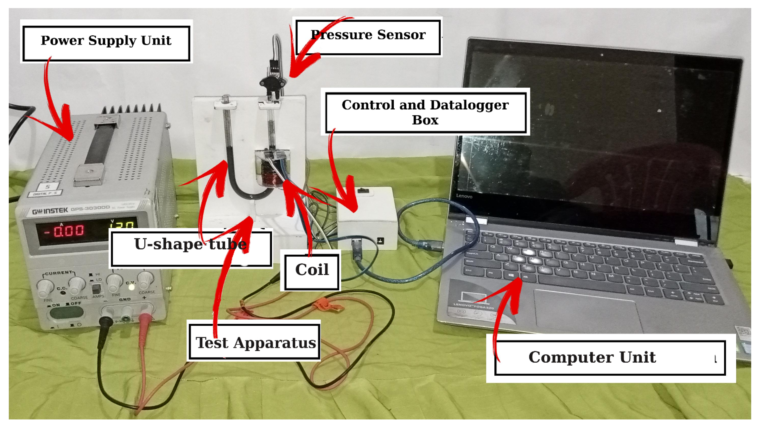
2. Materials and Methods

In a Poiseuille flow channel configuration, it is known that the magnetic field would generate a pressure difference and regulate the pressure drop, as occurs in the valve operating mode [28]. However, in a Poiseuille flow arrangement, the pressure difference is generated because the existing fluid flow is obstructed and thus, the measured pressure difference is identified as flow pressure drop occurs due to obstruction. The valve mode of the MRFs, for example, examined the magnitude of the pressure drop as a proportional contribution of the magnetic field strength and the yield stress of the fluid. On the other hand, the pressure measurement arranged in this paper is intended to observe the possibility of the magnetic field to generate pressure to the MRFs when it is at rest. Therefore the nature of the measurement is different from the measurement conducted at the valve mode arrangement.
In this study, the observation will be conducted using a U-shaped tube arrangement. The U-shaped tube method was chosen due to its simple pressure measurement process [29], as unequal pressure in the legs of the tube will result in different liquid levels, which indicate a pressure difference in the channel of the U-shaped tube. The U-shaped tube would be initially set at rest, with balanced pressure between both legs without a magnetic field. Once the liquid in both legs is level, the magnetic field is slowly applied by increasing the current input to the coil. The liquid levels are observed to see whether there were changes in the liquid levels in both legs when the magnetic field was applied. Figure 1 showed the reaction of the MRFs in the U-shaped tube when an external magnetic field was applied, and there is a clear difference between the liquid levels of both legs, which indicated a change in pressure. The level change, in this case, is caused by the magnetic induction to the magnetic particles immersed in the MRFs that provides magnetic force attraction to the particles until it each reach equilibrium position.
In order to quantify the observation, the magnetic field need to be estimated because it is not possible to insert the Gaussmeter probe in the U-shaped tube arrangement. The magnetic field estimation is conducted using FEMM an open-source software, 2-D finite element software widely used in magnetic analysis and simulations [11,30,31,32,33]. The FEMM simulation was carried out to simulate the magnetic circuits that exist in the theoretical model of the U-shaped tube apparatus. The material properties involved in the magnetic circuit are also used in the calculation, including the B-H curve values of the MRFs. To verify the accuracy of FEMM in estimating magnetic field strength a Gaussmeter test was also carried out on the upper surface of the coil on the axis of the coil hole, as shown in Figure 2a where measurements were possible. Figure 2b shows the observation point and magnetic field contour of the FEMM simulation. The observation point is 1 mm above the coil line due to the thickness of the bobbin that has been used. From the test result with Gaussmeter and FEMM Simulation, a comparison of results is obtained as shown in Figure 3. Based on the data obtained, that the simulation results are close to the measurement results, with an average error of 3%. Similar methods have been used in previous studies, such as in [11,30,33].
An experiment was then conducted with the research apparatus; a U-shaped tube was designed and made out of glass (Figure 4 and Figure 5). With the experimental apparatus model as shown in Figure 4, the volume of air trapped in the channel between MRFs and transducer is 1079.375 mm3.
The control variable of this study was the direct current (DC) supply, with a voltage of 12 volts and variable currents to generate varying magnetic field strengths for the MRFs. The current input variations were varied from 0.25 A to 2.00 A with 0.25 A intervals. An Arduino microcontroller unit (MCU), a laptop, and CuteCom graphical serial device terminal served as a data logger. An MPX5010DP differential pressure sensor (sensitivity 450 mV/Kpa ∼1 mV = 2.22 Pa) was used as the pressure data reader with a typical zero offset of 200 mV [34].
The MRF-122EG was poured into the U-shaped tube before the DC current is applied to the magnetic coil. The current input is alternated between 0.25 A, 0.50 A, 0.75 A, 1.00 A, 1.25 A, 1.50 A, 1.75 A, And 2.00 A every 10 s. The changes in pressure were monitored using the pressure sensor and recorded using the data logger at a sampling speed of 10 milliseconds (ms).

3. Results

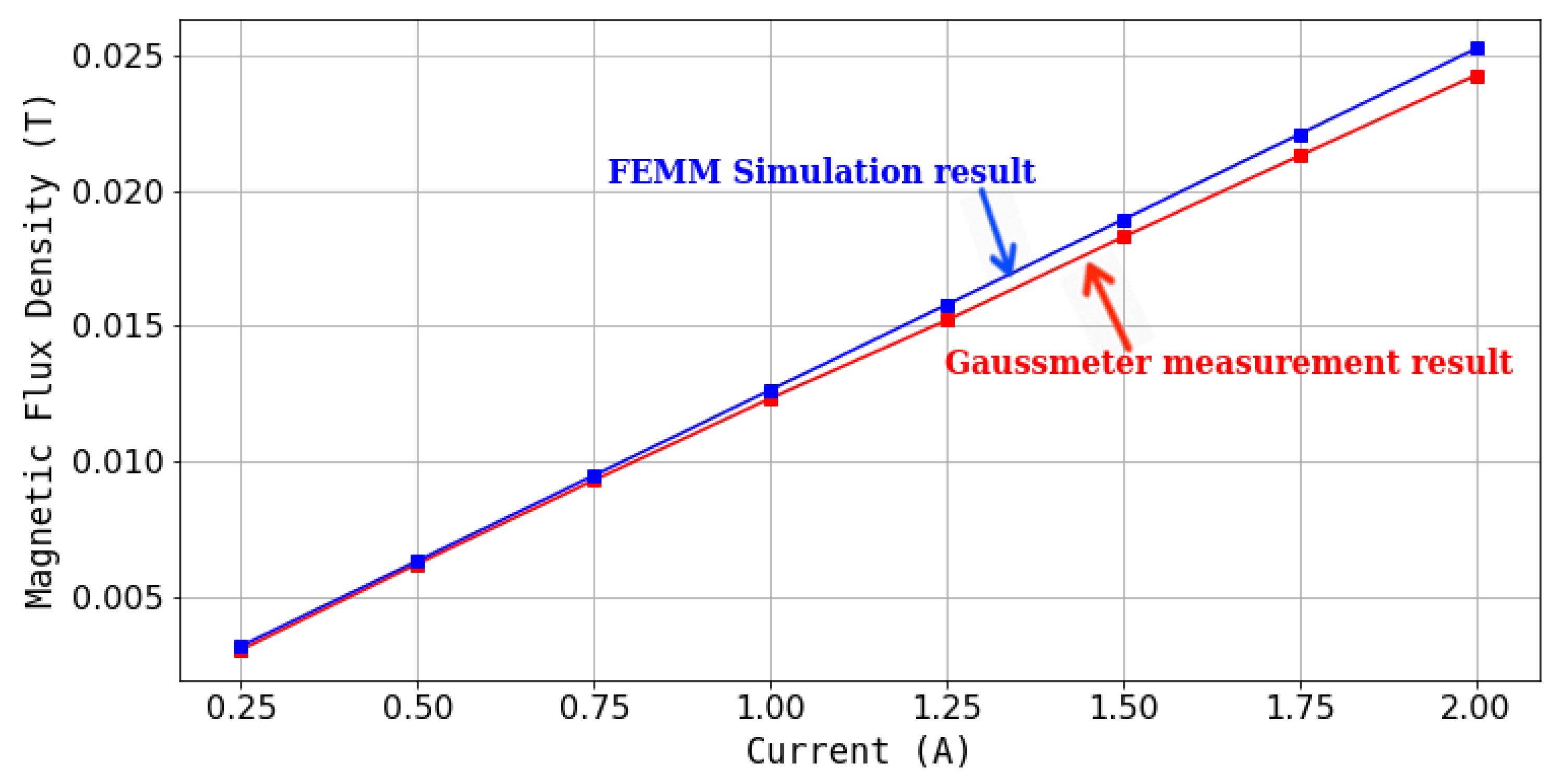
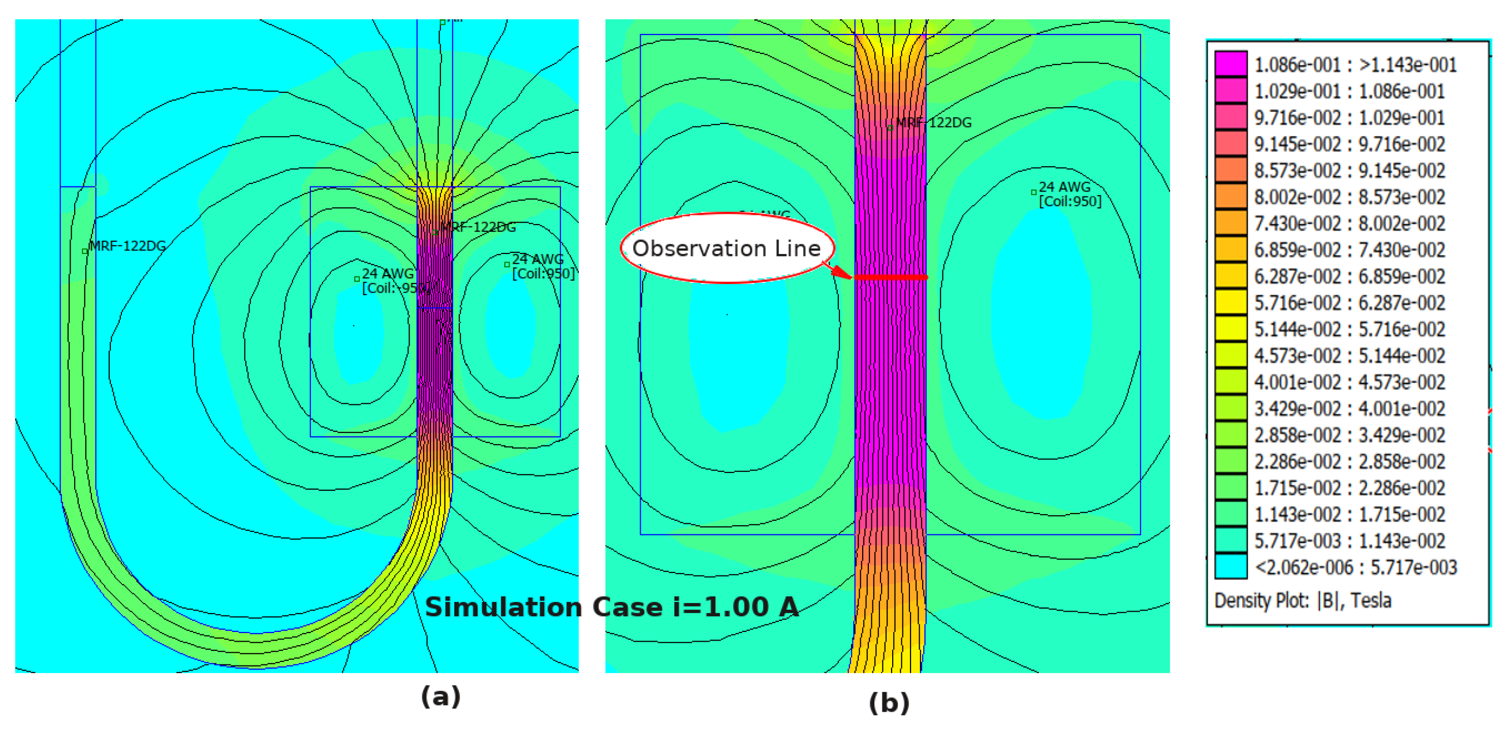
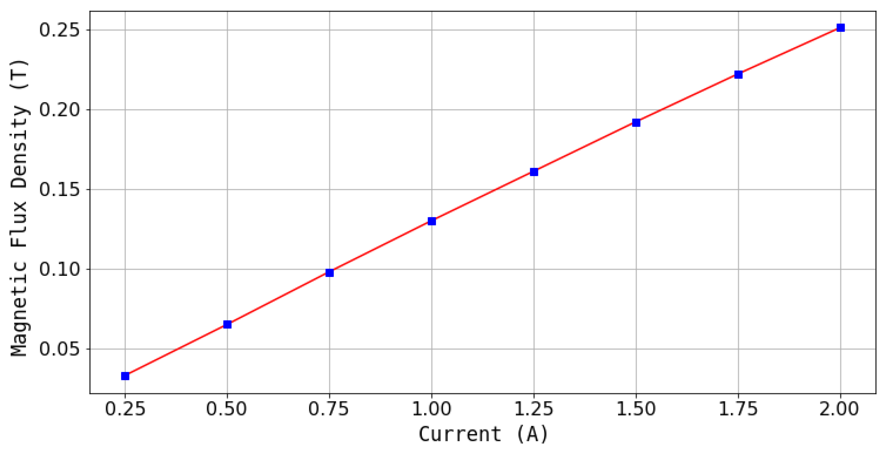
3.1. Simulation Results

The results of the FEMM simulation are shown in Figure 6a. The figure illustrates the magnetic flux generated around the electromagnetic coil, and the path coincides with the MRFs. According to the figure, it can be seen that the flux line coincides with the MRFs in a parallel direction, which is different from the common flux-fluid arrangement in the valve mode. As seen in Figure 6b, the observation line was used to point to the sampling section of the apparatus, in which the magnetic flux density data value will be collected and plotted from the simulation. According to the contour plot in Figure 6b, the magnetic flux density appears to be uniform along the mid-section of the y-axis.
The correlation curve between the applied current and the magnetic flux density at observasion line is shown in Figure 7. The figure shows that the magnetic flux density is linearly correlated with the current input with a slope of about 0.125 T/A.

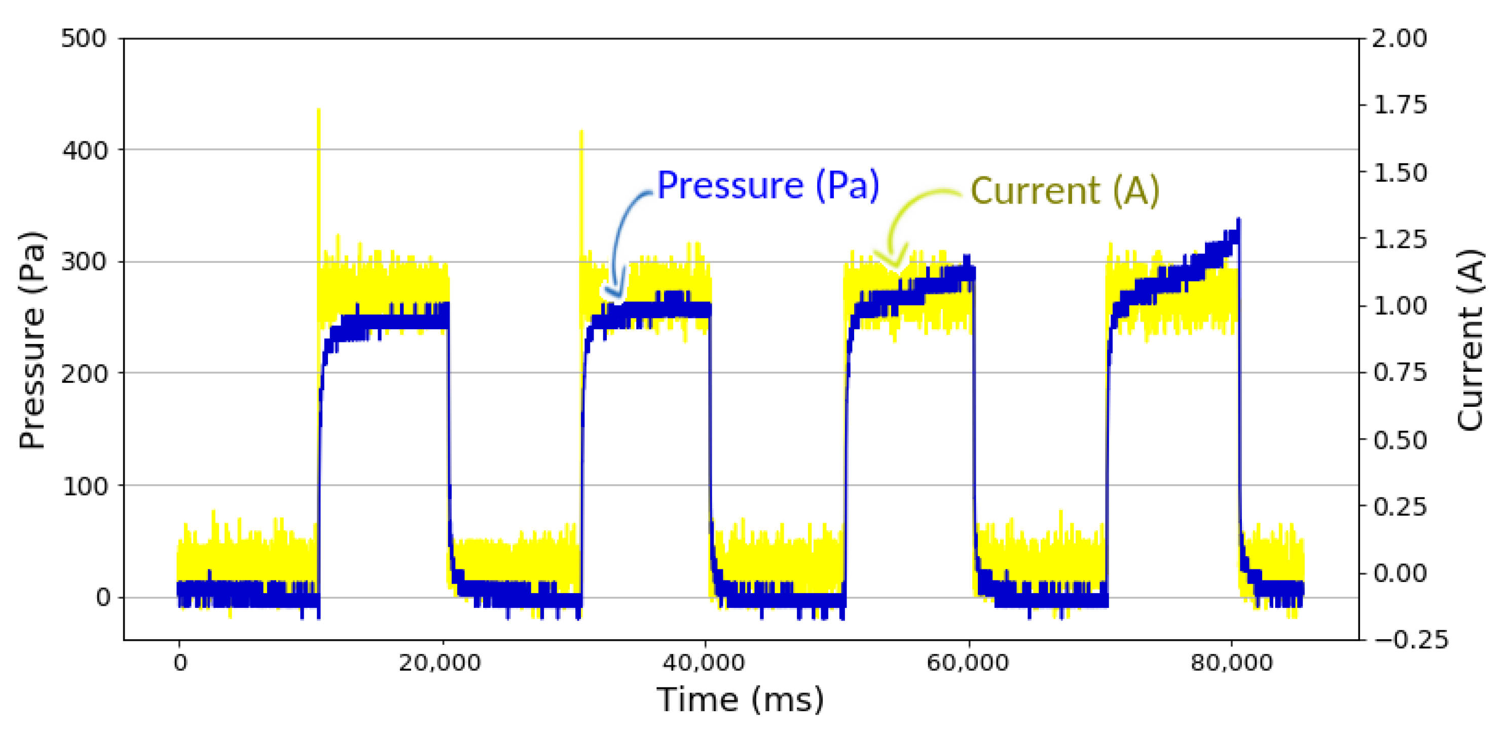
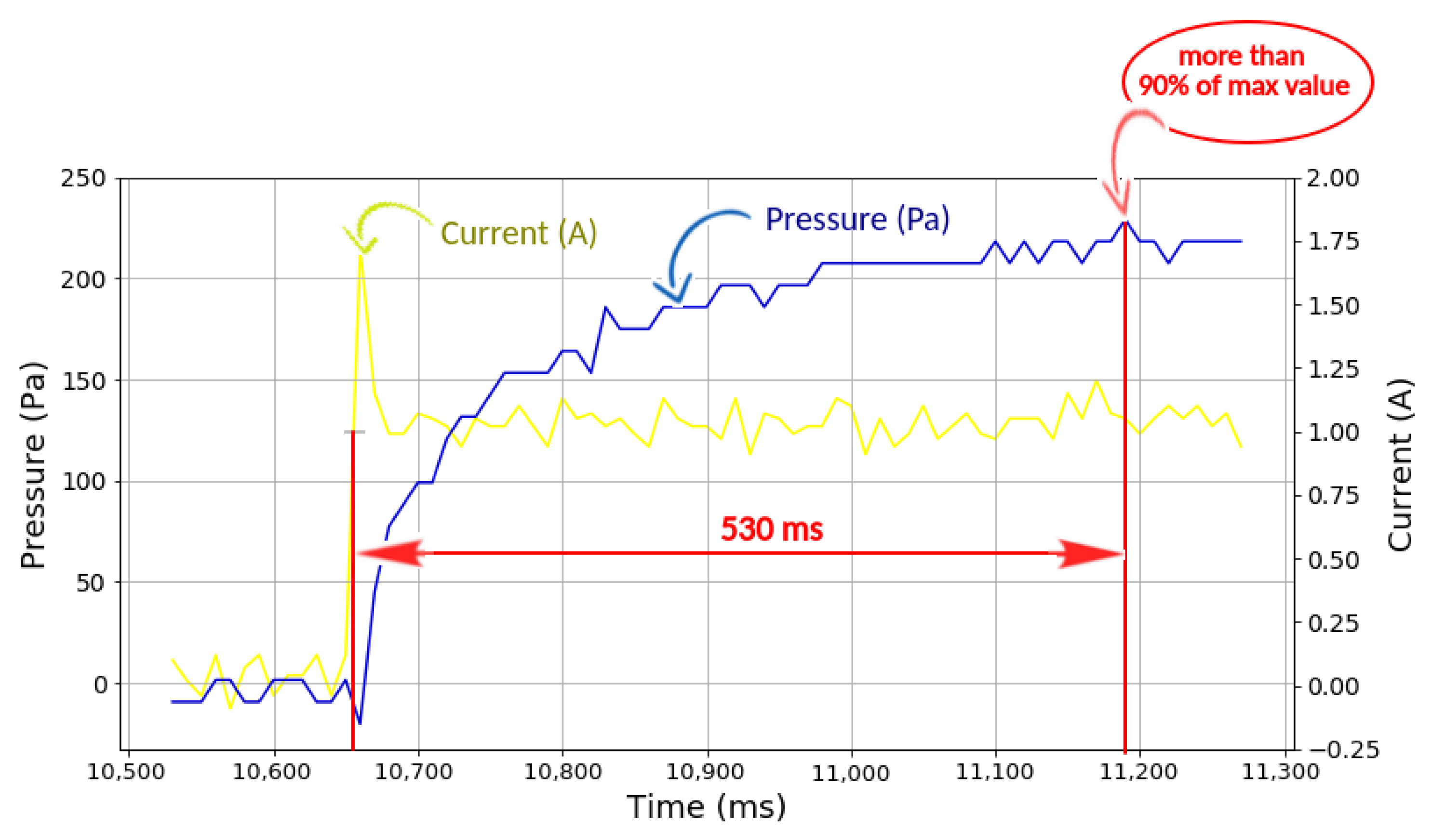
3.2. Experiment Results

The experimental results generally showed a significant effect of the magnetic field, which was represented by the amount of current input, to the change of MRFs pressure in the testing channel. For instance, Figure 8 shows the pressure values obtained at a current input of 1.00 A. The current input (yellow curved line) is seen in two states; the demagnetized state (Current = 0 A) and the magnetized state (Current = on); which results in changes of MRFs pressure. The MRFs pressure (blue curved line) is at its lowest when it is under a demagnetized state. But when the current input is turned on, the MRFs pressure increases proportionally to the input current.
As seen in Figure 9 the increase in MRFs pressure is consistent as the input current increases. At a lower current input, the change in MRFs pressure was relatively small as it only rose about 13.06 Pa to 18.39 Pa at 0.25 A current excitation. However, at a higher current input, the slope of MRFs pressure to current input is increased. For example, the average MRFs pressure was measured at about 267.80 Pa at 1.00 A of current excitation. Similar trends are still observed at input currents of 1.25 A, 1.50 A, 1.75 A, and 2.00 A with average changes in MRFs pressure of 517.16 Pa, 709.20 Pa, 904.64 Pa, 918.55 Pa, and 1020.01 Pa, respectively. The detail of overall changes in MRFs pressure during experiments is presented in Table 1.

4. Discussion

According to the Figure 8, the observations were carried out for several cycles where each cycle consist of 10 s demagnetized state and 10 s magnetized state. From the figure, it was seen that the pressure was relatively stable in the initial cycle, while the pressure tended to increase in the subsequent cycles. In Figure 8, it can be seen that there is an increase in the pressure slope in the continuation cycle, due to the accumulation of magnetic particles in the previous cycle. This case occurs because, during demagnetization, the magnetic particles cannot be completely re-distributed in the fluid.
It is evident that increases in the magnetic field have caused changes in the MRFs pressure. This is because the pressure sensor detects increases in the barometric pressure of the air above the MRFs. As seen in the boxplot shown in Figure 9, the MRFs pressure readings obtained during the experiment has only small deviations, which indicates the measurement consistency. The most apparent deviation in MRFs pressure occurred at an input current of 2.00 A. In general, the data was normally distributed except for the input current of 1.25 A, where the sole outlier is measured.
According to the results, a sudden change of slope was detected when current excitation reached 2.00 A. This condition is slightly different from the other region, which might be the result of the heat dissipated from the coil when excited with a high current. During the experiment, the temperature of the coil bobbin was found to exceed 60 °C when excited with a 2.00 A current. The heat generated will slightly increase the wire resistance and decreased coil performance which was indicated by an observed decrease in the current input to the coil after few cycles of measurement. A similar case was also reported in the previous work about thermal modeling on heated injectors [35]. During the first cycle, the change in MRFs pressure was measured at 1020.01 Pa as the input current reached 1.88 A. In the subsequent cycles, the change in MRFs pressure is decreased because the input current could only reach 1.85 A, 1.84 A, and 1.83 A.
Figure 10 depicts the graph obtained from the experiment at an input current of 1.00 A. It shows that the MRFs pressure had a relatively fast response time and reacted quickly to the input current. Response time is defined as the period that a sensor requires to reach 90% of the total signal response [36]. It took approximately 530 ms to get more values up to 90% of the maximum value. Meanwhile, it took 1810 ms; or less than 2 s, to get to the maximum value based on the data logger. It is evident that there is a trend for bigger changes in MRFs pressure when the strength of the magnetic field increased, which, in this case, was represented by the increased input current.

5. Conclusions

The experimental assessment to observe the effect of magnetic field induction on the fluid pressure of magnetorheological fluids (MRFs) has been conducted. The results showed that the MRFs fluid pressure could proportionally be increased with the increase of the magnetic field. The indication was observed visually with the fluid level change in the U-shaped tube and detected by the pressure sensor. Around 900 Pa of fluid pressure was recorded when the MRFs were subjected to 2.00 A current input to the electromagnet. According to the magnetic simulation, such an arrangement was estimated to produce about 0.25 T. The change of fluid pressure is positively correlated to the change of the magnetic field strentgh. Overall, the observation results indicate a strong relationship between MRFs fluid pressure and the magnetic field induction, which could pave the way to discovering a new MRFs operational mode.

Author Contributions

Conceptualization: P.J.W., U.U. and F.I.; Data curation: P.J.W.; Methodology: P.J.W., U.U. and F.I.; Supervision: E.P.B., U.U. and F.I.; Writing—original draft: P.J.W.; Writing—review & editing: P.J.W., E.P.B., U.U. and F.I. All authors have read and agreed to the published version of the manuscript.

Funding

Sebelas Maret University Doctoral Program Scholarship and Penelitian Unggulan UNS.

Institutional Review Board Statement

Not applicable.

Informed Consent Statement

Not applicable.

Data Availability Statement

The data presented in this study are available on request from the corresponding author. The data are not publicly available due to privacy.

Conflicts of Interest

The authors declare no conflict of interest.

Abbreviations

The following abbreviations are used in this manuscript:
AWGAmerican Wire Gauge
DCDirect Current
FEMMFinite Element Method Magnetics
MCUMicrocontroller Unit
MRFsMagnetorheological Fluids
PVCPolyvinyl Chloride

References

  1. Utami, D.; Ubaidillah; Mazlan, S.A.; Imaduddin, F.; Nordin, N.A.; Bahiuddin, I.; Abdul Aziz, S.A.; Mohamad, N.; Choi, S.-B. Material Characterization of a Magnetorheological Fluid Subjected to Long-Term Operation in Damper. Materials 2018, 11, 2195. [Google Scholar] [CrossRef] [Green Version]
  2. Imaduddin, F.; Mazlan, S.; Zamzuri, H. A design and modelling review of rotary magnetorheological damper. Mater. Des. 2013, 51, 575–591. [Google Scholar] [CrossRef]
  3. Bahiuddin, I.; Mazlan, S.A.; Shapiai, M.I.; Choi, S.-B.; Imaduddin, F.; Rahman, M.A.A.; Ariff, M.H.M. A new constitutive model of a magneto-rheological fluid actuator using an extreme learning machine method. Sens. Actuators A Phys. 2018, 281, 209–221. [Google Scholar] [CrossRef]
  4. Ubaidillah; Hudha, K.; Akmar, F.; Kadir, A. Modelling, characterisation and force tracking control of a magnetorheological damper under harmonic excitation. Int. J. Model. Identif. Control 2011, 13, 9–21. [Google Scholar] [CrossRef] [Green Version]
  5. Ubaidillah; Lenggana, B.; Son, L.; Imaduddin, F.; Widodo, P.; Harjana, H.; Doewes, R. A new magnetorheological fluids damper for unmanned aerial vehicles. J. Adv. Res. Fluid Mech. Therm. 2020, 73, 35–45. [Google Scholar] [CrossRef]
  6. Imaduddin, F.; Mazlan, S.A.; Ubaidillah; Idris, M.H.; Bahiuddin, I. Characterization and modeling of a new magnetorheological damper with meandering type valve using neuro-fuzzy. J. King Saud Univ.-Sci. 2017, 29, 468–477. [Google Scholar] [CrossRef]
  7. Gadekar, P.; Kanthale, V.S.; Khaire, N.D. Magnetorheological Fluid and its Applications. Int. J. Curr. Eng. Technol. 2017, 7, 32–37. [Google Scholar]
  8. Idris, M.H.; Imaduddin, F.; Ubaidillah; Mazlan, S.A.; Choi, S.-B. A concentric design of a bypass magnetorheological fluid damper with a serpentine flux valve. Actuators 2020, 9, 16. [Google Scholar] [CrossRef] [Green Version]
  9. Milecki, A.; Hauke, M. Application of magnetorheological fluid in industrial shock absorbers. Mech. Syst. Signal Process. 2012, 28, 528–541. [Google Scholar] [CrossRef]
  10. Hu, G.; Wu, L.; Li, L. Torque characteristics analysis of a magnetorheological brake with double brake disc. Actuators 2021, 10, 23. [Google Scholar] [CrossRef]
  11. Nya’Ubit, I.R.; Priyandoko, G.; Imaduddin, F.; Adiputra, D.; Ubaidillah. Torque characterization of t-shaped magnetorheological brake featuring serpentine magnetic flux. J. Adv. Res. Fluid Mech. Therm. 2020, 78, 85–97. [Google Scholar]
  12. Latha, H.; Pantangi, U.S.; Seetharamaiah, N. Design and manufacturing aspects of magneto-rheological fluid (mrf) clutch. Mater. Today Proc. 2017, 4, 1525–1534. [Google Scholar] [CrossRef]
  13. Jamalpour, R.; Nekooei, M.; Moghadam, A. Seismic response reduction of steel mrf using sma equipped innovated low-damage column foundation connection. Civ. Eng. J. 2017, 3, 1–14. [Google Scholar] [CrossRef] [Green Version]
  14. Dyke, S.J.; Spencer, B.F.; Sain, M.K.; Carlson, J.D. Seismic Response Reduction Using Magnetorheological Dampers. IFAC Proc. Vol. 1996, 29, 5530–5535. [Google Scholar] [CrossRef]
  15. Satria, R.R.; Ubaidillah, U.; Imaduddin, F. Analytical approach of a pure flow mode serpentine path rotary magnetorheological damper. Actuators 2020, 9, 56. [Google Scholar] [CrossRef]
  16. Abd Fatah, A.Y.; Mazlan, S.; Koga, T.; Zamzuri, H.; Imaduddin, F. Design of magnetorheological valve using serpentine flux path method. Int. J. Appl. Electromagn. Mech. 2016, 50, 29–44. [Google Scholar] [CrossRef]
  17. Sarkar, C.; Hirani, H.; Sasane, A. Magnetorheological smart automotive engine mount. Int. J. Curr. Eng. Technol. 2015, 5, 419–428. [Google Scholar]
  18. Zeinali, M.; Mazlan, S.A.; Choi, S.-B.; Imaduddin, F.; Hamdan, L.H. Influence of piston and magnetic coils on the field-dependent damping performance of a mixed-mode magnetorheological damper. Smart Mater. Struct. 2016, 25, 055010. [Google Scholar] [CrossRef]
  19. Sapinski, B. Simulation of an MR squeeze-mode damper for an automotive engine mount. In Proceedings of the 17th International Carpathian Control Conference (ICCC), IEEExplore, High Tatras, Slovakia, 29 May–1 June 2016; pp. 641–644. [Google Scholar]
  20. Yildirim, G.; Genc, S. Experimental study on heat transfer of the magnetorheological fluids. Smart Mater. Struct. 2013, 22, 085001. [Google Scholar] [CrossRef]
  21. Adiputra, D.; Rahman, M.A.A.; Bahiuddin, I.; Ubaidillah; Imaduddin, F.; Nazmi, N. Sensor number optimization using neural network for ankle foot orthosis equipped with magnetorheological brake. Open Eng. 2021, 11, 91–101. [Google Scholar] [CrossRef]
  22. Bhavsar, P.; Unune, D.R. Magnetorheological Polishing Tool for Nano-Finishing of Biomaterials. In Proceedings of the 10th International Conference on Precesion, Meso, Micro and Nano Engineering, Chennai, India, 7–9 December 2017; pp. 6–10. [Google Scholar]
  23. Purnomo, E.D.; Ubaidillah; Imaduddin, F.; Yahya, I.; Mazlan, S. Preliminary experimental evaluation of a novel loudspeaker featuring magnetorheological fluid surround absorber. Indones. J. Electr. Eng. Comput. 2020, 17, 922–928. [Google Scholar] [CrossRef] [Green Version]
  24. Dyana Kumara, K.A.; Ubaidillah, U.; Priyandoko, I.Y.G.; Wibowo, W. Magnetostatic Simulation in a Novel Magnetorheological Elastomer Based Loudspeaker Surround. In Proceedings of the 2019 6th International Conference on Electric Vehicular Technology (ICEVT), Bali, Indonesia, 18–21 November 2019; pp. 295–299. [Google Scholar]
  25. Ahamed, R.; Choi, S.-B.; Ferdaus, M.M. A state of art on magneto-rheological materials and their potential applications. J. Intell. Mater. Syst. Struct. 2018, 29, 2051–2095. [Google Scholar] [CrossRef]
  26. Rahman, M.; Chao, O.; Julai, S.; Ferdaus, M.M.; Ahamed, R. A review of advances in magnetorheological dampers: Their design optimization and applications. J. Zhejiang Univ. Sci. A 2017, 18, 991–1010. [Google Scholar] [CrossRef]
  27. de Vicente, J.; Klingenberg, D.J.; Hidalgo-Alvarez, R. Magnetorheological fluids: A review. Soft Matter 2011, 7, 3701–3710. [Google Scholar] [CrossRef]
  28. Ostadfar, A. Chapter 1—Fluid Mechanics and Biofluids Principles. In Biofluid Mechanics; Ostadfar, A., Ed.; Academic Press: London, UK, 2016; pp. 1–60. [Google Scholar]
  29. Vijayaraghavan, G.K.; Sundaravalli, S. Pressure and Pressure Measuring Devices. In Fluid Mechanics and Machinery; Lakshmi Publications: Chennai, India, 2018; ISBN 978-93-831030-8-9. [Google Scholar]
  30. Ubaidillah; Wirawan, J.W.; Lenggana, B.W.; Purnomo, E.D.; Widyarso, W.; Mazlan, S.A. Design and Performance Analysis of Magnetorheological Valve for Upside-Down Damper. J. Adv. Res. Fluid Mech. Therm. 2019, 63, 164–173. [Google Scholar]
  31. Yatchev, I.; Gueorgiev, V.; Ivanov, R.; Hinov, K. Simulation of the dynamic behaviour of a permanent magnet linear actuator. Facta Univ.-Ser. Electron. Energy 2010, 23, 37–43. [Google Scholar] [CrossRef] [Green Version]
  32. Białek, M.; Nowak, P.; Lindner, T.; Wyrwał, D. FEMM Examination of the Gripper with Magnetorheological Cushion. In Proceedings of the 2020 International Conference Mechatronic Systems and Materials (MSM), Bialystok, Poland, 1–3 July 2020; pp. 1–5. [Google Scholar]
  33. Ubaidillah; Lenggana, B.W. Finite Element Magnetic Method for Magnetorheological Based Actuators. In Finite Element Methods and Their Applications; IntechOpen: London, UK, 2020; pp. 1–18. [Google Scholar] [CrossRef]
  34. Freescale Semiconductors Inc. Technical Data Sheet: MPXV5010DP, 0 to 10 kPa, Differential, Gauge, and Absolute, Integrated, Pressure Sensors; Freescale Semiconductors Inc.: Austin, TX, USA, 2012. [Google Scholar]
  35. Volpato, O. Thermal Modeling of Heated Injectors; SAE Technical Papers 2011-36-0087; SAE: Warrendale, PA, USA, 2011. [Google Scholar] [CrossRef]
  36. Arafat, M.M.; Dinan, B.; Akbar, S.A.; Haseeb, A.S.M.A. Gas sensors based on one dimensional nanostructured metal-oxides: A review. Sensors 2012, 12, 7207–7258. [Google Scholar] [CrossRef]
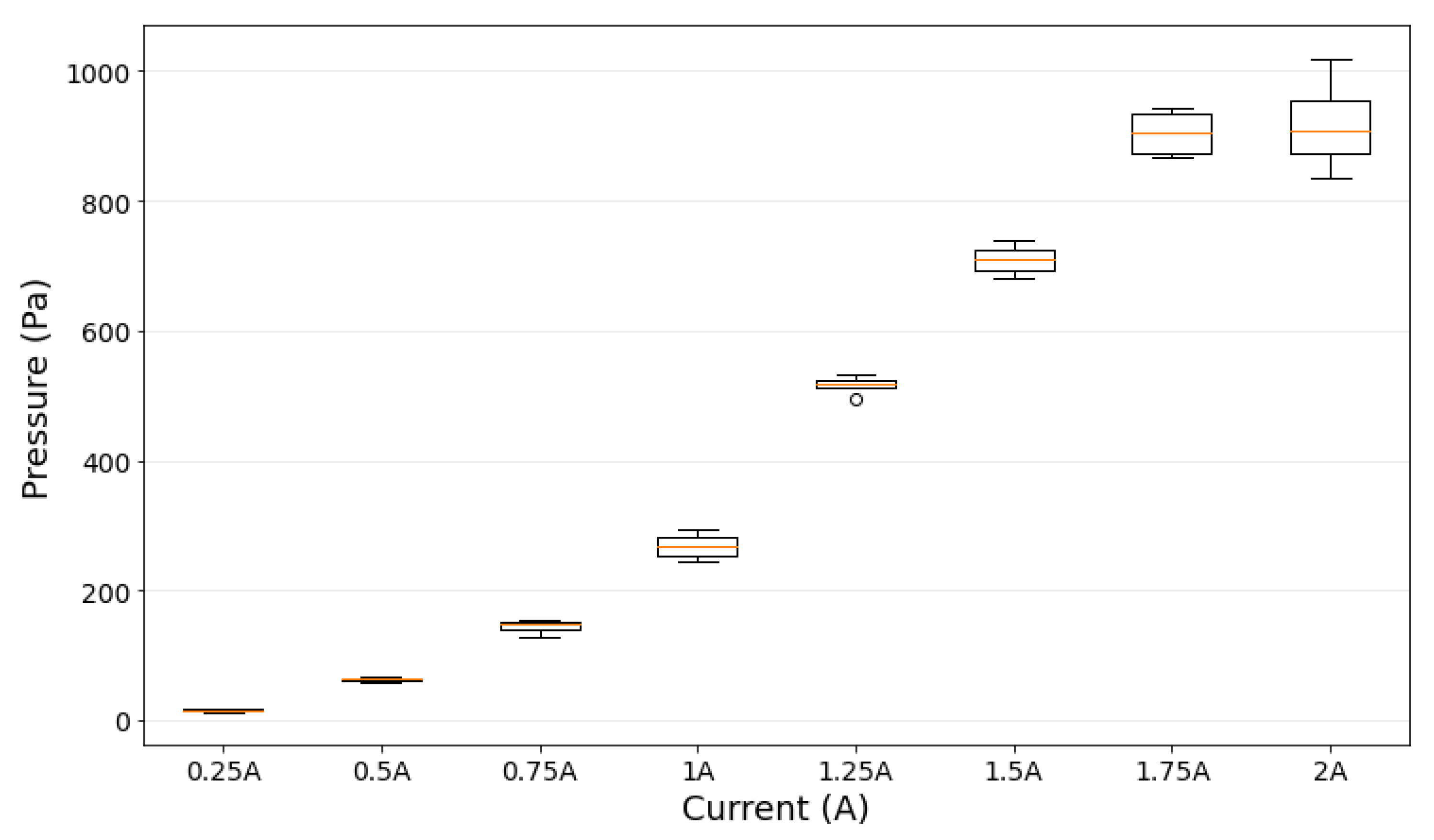
Figure 1. Different MRFs levels in both legs indicating a pressure change.
Applsci 11 09807 g001
Figure 2. FEMM verification setup, (a) measurement setup (b) FEMM Simulation contour plot.
Applsci 11 09807 g002
Figure 3. Comparison Results of Gaussmeter Measurement and FEMM Simulation.
Applsci 11 09807 g003
Figure 4. The U-shaped tube and other testing equipment.
Applsci 11 09807 g004
Figure 5. The research apparatus.
Applsci 11 09807 g005
Figure 6. (a) Results of the FEMM software simulation (current input = 1 A); (b) The observation line that was used in the simulation.
Applsci 11 09807 g006
Figure 7. A graph of the correlation between current and magnetic flux density in the FEMM software simulation.
Applsci 11 09807 g007
Figure 8. Experiment results of MRFs pressure at an input current of 1.00 A.
Applsci 11 09807 g008
Figure 9. A box plot of MRFs pressure (Pascal) and input current (Ampere).
Applsci 11 09807 g009
Figure 10. Changes in MRFs pressure at an input current of 1.00 A.
Applsci 11 09807 g010
Table 1. Experiment Data.
Current Input (A)0.250.500.751.001.251.501.752.00
∆Pmin (Pa)13.0658.98129.17244.49496.04679.79867.36835.50
∆Pmax (Pa)18.3965.91155.64292.53533.77739.02942.501020.01
∆Pavg (Pa)15.5362.80144.77267.80517.16709.20904.64918.55
∆Pmedian (Pa)15.3463.16147.14267.09519.42708.99904.34909.34
Std Deviation2.683.1211.5221.2915.6325.8538.3778.84
Note: ∆Pmin is the minimum pressure change that occurs during magnetization at the observation cycle at each given current, ∆Pmax is the maximum pressure change that occurs during magnetization at the observation cycle at each given current, ∆Pavg is the average pressure change that occurs during magnetization at the observation cycle, Std Deviation is the standard deviation of the measured pressure.
Publisher’s Note: MDPI stays neutral with regard to jurisdictional claims in published maps and institutional affiliations.

