Adaptive Predictive Functional Control of X-Y Pedestal for LEO Satellite Tracking Using Laguerre Functions

Featured Application

The developed control algorithm can be used in X-Y pedestals for the tracking of the low earth orbit (LEO) satellites.

Abstract

In this paper, Predictive Functional Control (PFC) is used for X-Y pedestal control for LEO satellite tracking. According to the nonlinear characteristics of the X-Y pedestal and pedestal model variation caused by its operating point change, the use of system identification algorithm, which is based on special types of orthonormal functions known as Laguerre functions, is presented. This algorithm is combined with PFC to obtain a novel adaptive control algorithm entitled Adaptive Predictive Functional Control (APFC). In this combination, Laguerre functions are utilized for system identification, while the PFC is the control law. An interesting feature of the proposed algorithm is its desirable performance against the interference effect of channel X and channel Y. The proposed APFC algorithm is compared with Proportional Integral Derivative (PID) controller using simulation results. The results confirm that the proposed controller improves the performance in terms of the pedestal model variations; that is, the controller is capable of adapting to the model changes desirably.

1. Introduction

Pedestals play a substantial role in satellite tracking, as they are important modules in satellite tracking stations. The antenna in the pedestal is, ideally, in constant, uninterrupted orientation with the signal source. Because either the target, the platform, or both are in constant motion, the pedestal may be adjusted by the associated motors so as to ensure that the payload has continuous and uninterrupted tracking of the source [1]. The best quality of data reception is obtained when the telemetry signal is stronger, i.e., where the satellite is closest to the ground station [2]. The most common and well-known type of pedestal is the Elevation over Azimuth (El/Az). The main disadvantage of the El/Az pedestals is their inability to track the target near their zenith position. When the satellite is directly overhead, the El/Az system will stop tracking at zenith, because at this point the azimuth angle after zenith is 180 degrees different from the azimuth angle immediately prior to zenith. To continue tracking, the azimuth motor must turn the payload nearly 180 degrees within a brief period of time while the satellite crosses the zenith position. However, even the fastest motors are unable to turn the payload 180 degrees in non-zero time [1,2]. In the late of 1990s, another type of pedestal known as the X-Y pedestal (which has been referred to by a variety of terms, including: X over Y; cross elevation over elevation; traverse over elevation; cross level over elevation; dual elevation; two-axis zenith search) was designed and manufactured so as to receive satellite data in fixed and mobile earth stations. An X-Y pedestal system has the ability to rotate about the X and Y axes, which are substantially orthogonal to each other but not necessarily coplanar [1]. In comparison to common El/Az structures, the design and implementation of X-Y pedestals is more complex due to their different mechanical and control features. However, X-Y pedestals are considered to be a very suitable option for the design and construction of small and medium sized pedestals [3,4], due to the possibility of applying cheaper equipment, obtaining greater reliability, requiring less maintenance, and the feasibility of achieving high accuracy. In this line, X-Y Pedestals are considered as a suitable solution for Low Earth Orbit (LEO) satellite tracking, especially in the tracking of the target near their zenith position where the well-known El/Az pedestals cannot track the target. Despite all of the benefits of X-Y pedestals, control of them remains a challenging task. Some of the advantages and applications of X-Y mounts have been described in [5,6,7].

The PID controllers [8,9,10,11] were the first choice for X-Y pedestal control in satellite tracking, as was the case for many industrial applications. The nonlinear and multivariable nature of the X-Y pedestal and the variations of the operating point (caused by the changes in the pedestal center of gravity) result in weak performance of these controllers. Hence, the application of more complex controllers became necessary [12,13,14]. Model predictive controllers [15,16,17] are particularly appropriate for LEO satellite tracking due to the specified orbit of the LEO satellites, which can be realized by solving the satellite motion equations or through satellite motion simulation software. Predictive Functional Control (PFC) [18] is one of the model predictive controllers, and is characterized by two distinctive features: the control signal is structured as a linear combination of predetermined basis functions and the concept of coincidence points helps to evaluate the cost function on the prediction horizon. PFC is convenient for fast processes and nonlinear systems [15,18]. Many applications of PFC have been reported in recent years in industrial processes [19,20,21,22].

On the other hand, since the system model is nonlinear and time-variant (as a result of the satellite motion being followed by the antenna motion), applying online system identification methods and adaptive control [23] are considered to be appropriate options in order to achieve a desirable performance.

In this paper, unstructured system identification based on Laguerre functions [24,25,26,27,28,29,30,31] is combined by predictive functional control to achieve an adaptive predictive functional control algorithm. In this line, PFC is the control law, while the Laguerre functions are utilized for system modeling. Similar combinations have been reported in [32,33]. In [32], some different methods for the tuning of PFC parameters have been presented. In addition, in [33], Laguerre functions have been utilized to improve the performance of PFC. The main advantages of the proposed algorithm are high speed, low computational effort, simple control, and desirable accuracy in the satellite tracking.

In [12,13], similar works have been conducted for the control of X-Y pedestals. In [12], two forms of predictive laws, named Generalized Predictive Control (GPC) and Generalized Incremental Predictive Control (GIPC), have been used for pedestal control. Model Predictive Control (MPC) and GPC have been utilized to control the X-Y pedestal in [13] and the results were compared with PI control. In contrast to this work, the control laws applied in [12,13] are not adaptive. Therefore, the proposed control laws are not suitable for handling changes in the model of the system. Furthermore, GPC, MPC, and GIPC are more complicated for implementation in comparison to PFC.

This paper is organized as follows: the structure of the X-Y pedestal and its governing differential equations are presented in Section 2.1. In Section 2.2, Laguerre functions, which are utilized for unstructured system identification, are introduced. Section 2.3 describes the predictive functional control. The procedure for achieving the optimal control law is given in Section 2.4. Section 2.5 presents the stability analysis of the closed-loop system. The simulation results of the proposed control scheme are presented in Section 3. Furthermore, the APFC algorithm, based on the Laguerre functions, is compared with the PID controller. Finally, the main results are concluded in Section 4.

2. Materials and Methods

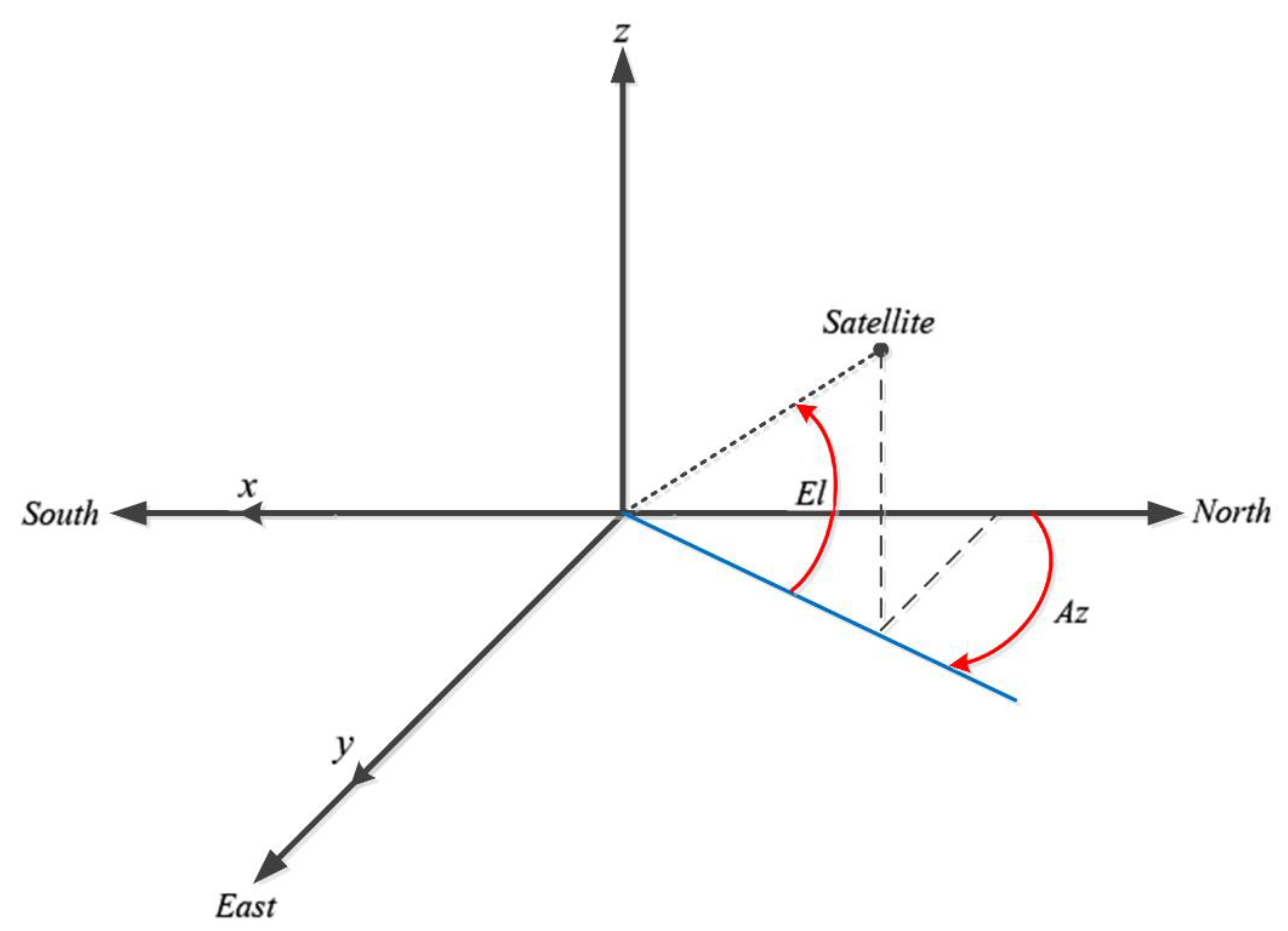
2.1. X-Y Pedestal System

X-Y pedestals are generally used for the tracking of LEO satellites. Their capability of tracking the satellite in the zenith pass area is their main advantage.

The coordinates of a satellite are usually expressed in terms of the elevation and azimuth angles. The aim is to determine the desirable angles in joint space for directing the antenna toward the satellite. The joint angles are entitled ${\theta }_1$ and ${\theta }_2$. In fact, the satellite trajectory is expressed by the elevation and azimuth angles at any moment, as illustrated in Figure 1.

As a result, if the satellite trajectory is expressed by elevation ($El$) and azimuth ($Az$) angles, the required joint angles could be extracted. For this purpose, the mapping given in (1) is utilized, which maps the elevation and azimuth angles to the joint angles ${\theta }_1$ and ${\theta }_2$ [2,7,12,13]. In this expression, ${\theta }_1$ and ${\theta }_2$ are $–Y$ and $X$ angles, respectively.

$$\begin{gathered} sin\left(Az\right)cos\left(El\right)=sin{\theta }_2\stackrel{ }{\Rightarrow }{\theta }_2={sin}^{-1}\left[sin\left(Az\right)cos\left(El\right)\right] \\ \begin{array}{c}cos\left(Az\right)cos\left(El\right)=sin{\theta }_{1}cos{\theta }_2\hfill \\ sin\left(El\right)=cos{\theta }_{1}cos{\theta }_2 \hfill \end{array}\}\stackrel{ }{\Rightarrow }{\theta }_1={\tan }^{-1}\left[\frac{cos\left(Az\right)cos\left(El\right)}{sin\left(El\right)}\right] \\ -\frac{\pi }{2}<{\theta }_1, {\theta }_2<+\frac{\pi }{2} \end{gathered}$$

(1)

The Euler–Lagrange method is used to extract the dynamic equations of the pedestal. In this method, the kinetic and potential energies of the system are calculated. The X-Y pedestal is modeled by the following differential equation [2,7]:

$$\left[M\left(\underset{\_}{\theta }\right)\right]\left[\begin{array}{c}{\ddot{\theta }}_1\\ {\ddot{\theta }}_2\end{array}\right]+\left[C\left(\underset{\_}{\theta },\underset{\_}{\dot{\theta }}\right)\right]+\left[G\left(\underset{\_}{\theta }\right)\right]=\left[\begin{array}{c}{\tau }_1\\ {\tau }_2\end{array}\right]$$

(2)

In (2), ${\tau }_1$ and ${\tau }_2$ are the input torques for $Y$ and $X$ axes, respectively. According to (2), it is clear that the X-Y pedestal is a Multiple-Input Multiple-Output (MIMO) system, where the interference effect exists as well. For detailed information about the elements of the matrices in (2), see Appendix A and [2,7].

2.2. Unstructured System Identification Using Laguerre Functions

Laguerre functions are a complete orthonormal set in $L_2 \left(0,\infty \right)$ space, and they are particularly popular due to their simple realization. These functions are defined as a functional series [27,28,30,31]:

$${\Phi }_i\left(t\right)=\sqrt{2p}\frac{e^{pt}}{\left(i-1\right)!}\frac{d^{i-1}}{d{t}^{i-1}}\left[t^{i-1}.e^{2pt}\right] , i=1,2,\dots ,\infty$$

(3)

where $p$ is a constant called time scaling factor, and $t\in \left[0,\infty \right)$ is a time variable. The Z-transform of the Laguerre functions is [27,28,30,31]:

$${\Phi }_i\left(z\right)=\mathcal{Z}\left\{{\Phi }_i\left(t\right)\right\}=\frac{\sqrt{1-p^2}}{1-p{z}^{-1}}{\left(\frac{z^{-1}-p}{1-p{z}^{-1}}\right)}^{i-1}, i=1,2,\dots ,\infty$$

(4)

Any open-loop stable system can be approximated by $n$ order Laguerre series as [30,31]:

$$Y_m\left(z\right)={\displaystyle \sum }_{i=1}^n{C}_i{\Phi }_i\left(z\right)U\left(z\right)={\displaystyle \sum }_{i=1}^n{C}_i{l}_i\left(z\right)$$

(5)

Among the different methods for expressing the Laguerre ladder network, the state space form is more suitable for system identification. Hence, the system outputs could be derived in the time domain directly. Using Laguerre functions, the system can be expressed in the discrete form as [27,28,30]:

$$\begin{gathered} L\left(k+1\right)=AL\left(k\right)+Bu\left(k\right) \\ \mathrm{y}\left(k\right)=CL\left(k\right) \end{gathered}$$

(6)

In (6), $L\left(k\right)$ is a $N\times 1$ state vector and $u\left(k\right)$ denotes the system input. $A$ is a $N\times N$ lower triangular system matrix. $y\left(k\right)$ is the system output. $B$ and $C$ are the coefficient vector of the control input and the observer coefficient vector, respectively. Considering $T$ as the system sampling period and:

$$\begin{gathered} {\tau }_1=\exp \left(-pT\right) \\ {\tau }_2=T+\frac{2}{p}\left(\exp \left(-pT\right)-1\right) \\ {\tau }_3=-T\exp \left(-pT\right)-\frac{2}{p}\left(\exp \left(-pT\right)-1\right) \\ {\tau }_4=\frac{\sqrt{2p}\left(1-{\tau }_1\right)}{p} \\ \alpha ={\tau }_1{\tau }_2+{\tau }_3 \end{gathered}$$

(7)

The system matrices are derived as:

$$\begin{gathered} A=\left[\begin{array}{cccc}{\tau }_1& 0& 0& 0\\ -\frac{\alpha }{T}& {\tau }_1& \dots & 0\\ ⋮& \ddots & \ddots & ⋮\\ \frac{{\left(-1\right)}^{N-1}{\tau }_2^{N-2}\alpha }{T^{N-1}}& \cdots & -\frac{\alpha }{T}& {\tau }_1\end{array}\right] \\ B={\left[{\tau }_4 \left(-\frac{{\tau }_2}{T}\right){\tau }_4 \dots {\left(-\frac{{\tau }_2}{T}\right)}^{N-1}{\tau }_4 \right]}^T \\ L\left(k\right)={\left[l_1\left(k\right) l_2\left(k\right) \dots l_N\left(k\right)\right]}^T \\ C=\left[c_1 c_2 \dots c_N\right] \end{gathered}$$

(8)

Elements of $A$ and $B$ are determined off-line, hence reducing the computational burden considerably. The Recursive Least Squares (RLS) [23,34,35] algorithm is utilized for online determining of the elements of the $C$ vector:

$$\begin{gathered} C\left(k\right)=C\left(k-1\right)+{\left\{M\left(k\right)\left[y\left(k\right)-C\left(k-1\right)L\left(k-1\right)\right]\right\}}^T \\ M\left(k\right)=\frac{P\left(k-1\right)L\left(k-1\right)}{\lambda +L^T\left(k-1\right)P\left(k-1\right)L\left(k-1\right)} \\ P\left(k\right)=\frac{1}{\lambda }\left[P\left(k-1\right)-M\left(k\right)L^T\left(k\right)P\left(k-1\right)\right] \end{gathered}$$

(9)

where $0<\lambda \le 1, \lambda$ is the forgetting factor in RLS algorithm.

The following assumptions are considered for the system:

A.1. $C$ is bounded and the state space of the system is stable ($p>0$), observable, and controllable.

A.2. Laguerre functions are an accurate description of the system.

2.3. Predictive Functional Control (PFC)

The principle of the PFC is similar to that of classic predictive control. Both use the same model for predicting the future of the system output. In predictive functional control, the control law structure is considered as a linear combination of a set of base functions. Hence, the weight coefficients of these base functions should be calculated. Selection of base functions depends on the process features and the desired reference input. The control law can be considered as [28]:

$$u\left(k+i\right)={\displaystyle \sum }_{n=1}^N{\mu }_n{u}_{bn}\left(i\right)$$

(10)

In (10), ${\mu }_n$ denotes the weight coefficients of the base functions in linear combination, where $N$ specifies the number of the base functions. $u_{bn} \left(i\right)$ represents the base functions’ values at the moment $t=k+i$. As stated before, base functions are selected according to the process nature and the reference input. Generally, step, ramp, and parabolic functions are utilized. In most cases, using step and ramp functions together is sufficient [28]:

$$u\left(k+i\right)={\mu }_1\left(k\right)+{\mu }_2\left(k\right)\times i$$

(11)

The reference trajectory is calculated by an exponential relationship [28]:

$$y_r\left(k+i\right)=w\left(k+i\right)-{\lambda }^i\left[w\left(k\right)-y\left(k\right)\right]$$

(12)

where $i=1,\dots ,H_i$ is the number of total coincidence points. $y_r \left(k+i\right)$ denotes the reference trajectory values at the moment $t=k+i$. $w\left(k\right)$ represents the set point and $y\left(k\right)$ is the output of the process. ${\lambda }^i=exp\left(-T_s⁄T_r\right)$ in which $T_s$ and $T_r$ are the sampling period and the expected time for a response to the reference trajectory, respectively. Accordingly, by combining (6) and (11), the system future output could be calculated as follows [28]:

$$y_m\left(k+i\right)=C{A}^{i}L\left(k\right)+C\left[A^{i-1}+A^{i-2}+\dots +I\right]B{\mu }_1\left(k\right)+C\left[A^{i-2}+2A^{i-3}+\dots +\left(i-1\right)I\right]B{\mu }_2\left(k\right)$$

(13)

In (13), $y_m \left(k+i\right)$ is the model output at the moment $t=k+i$. $e\left(k+i\right)$ represents the predicted error, which is the difference between the model and the process outputs at the moment $t=k+i$. $e\left(k+i\right)$ is derived by the following polynomial using filtered observations on the past horizon:

$$e\left(k+i\right)=y\left(k\right)-y_m\left(k\right)$$

(14)

2.4. PFC Law

For determination of ${\mu }_1 \left(k\right)$ and ${\mu }_2 \left(k\right)$ in the control law (11), consider the cost function (15):

$$J={\displaystyle \sum }_{i=H_1}^{H_2}{\left[y_m\left(k+i\right)+e\left(k+i\right)-y_r\left(k+i\right)\right]}^2$$

(15)

If the first and the last points of the prediction horizon are considered, (15) is written as follows:

$$J={\left[y_m\left(k+H_1\right)+e\left(k+H_1\right)-y_r\left(k+H_1\right)\right]}^2+{\left[y_m\left(k+H_2\right)+e\left(k+H_2\right)-y_r\left(k+H_2\right)\right]}^2$$

(16)

Optimization of (16) respect to ${\mu }_1\left(k\right)$ and ${\mu }_2\left(k\right)$ results in:

$$u\left(k\right)={\mu }_1\left(k\right)=S_{y}y\left(k\right)+S_{L}L\left(k\right)+S_{w}w\left(k\right)$$

(17)

where:

$$\begin{gathered} S_y=Q\left(Q_3{M}_{12}-Q_2{M}_{11}\right)\left(1-{\alpha }^{H_1}\right)+Q\left(Q_3{M}_{22}-Q_2{M}_{21}\right)\left(1-{\alpha }^{H_2}\right) \\ {S}_L=Q\left(Q_3{M}_{12}-Q_2{M}_{11}\right)C\left(A^{H_1}-I\right)+Q\left(Q_3{M}_{22}-Q_2{M}_{21}\right)C\left(A^{H_2}-I\right) \\ {S}_w=-S_y \\ {Q}_1=M_{11}^2+M_{21}^2 \\ {Q}_2=M_{12}^2+M_{22}^2 \\ {Q}_3=M_{11}{M}_{12}+M_{21}{M}_{22} \\ Q=\frac{1}{Q_1{Q}_2-Q_3^2} \\ {M}_{11}=C\left(A^{H_1-1}+A^{H_1-2}+\dots +I\right)B \\ {M}_{12}=C\left(A^{H_1-2}+2A^{H_1-3}+\dots +\left(H_1-1\right)I\right)B \\ {M}_{21}=C\left(A^{H_2-1}+A^{H_2-2}+\dots +I\right)B \\ {M}_{22}=C\left(A^{H_2-2}+2A^{H_2-3}+\dots +\left(H_2-1\right)I\right)B \end{gathered}$$

(18)

It should be noted that ${\mu }_1\left(k\right)$ can be determined only if $Q$ exists. Hence, the free parameters of the controller, $H_1$ and $H_2$ should be selected carefully to ensure the existence of $Q.$ Another point in predictive functional control is that the number of coincidence points is arbitrary. By considering two coincidence points, the first point determines the beginning of the predictive horizon and the second one specifies the end of the predictive horizon.

2.5. Stability Analysis

Using the assumption (A.2) mentioned in Section 2.2 and expressions (6) and (17), the equation of the closed-loop state space model can be written as:

$$L\left(k+1\right)=A_{c}L\left(k\right)+B{S}_{w}w\left(k\right)$$

(19)

In (19), $A_c=A+B{S}_L+B{S}_{y}C$. Based on assumption (A.1) in Section 2.2, it is obvious that the elements of the $C$ vector are bounded. The $A$ matrix and $B$ vector of the model are time-invariant. According to (18), $S_L$, $S_w$, and $S_y$ are bounded as well. The values of set points, $w\left(k\right)$ are assumed to be always bounded. By considering linear control law and using discrete form of Lyapunov stability theorem, closed-loop poles can be computed.

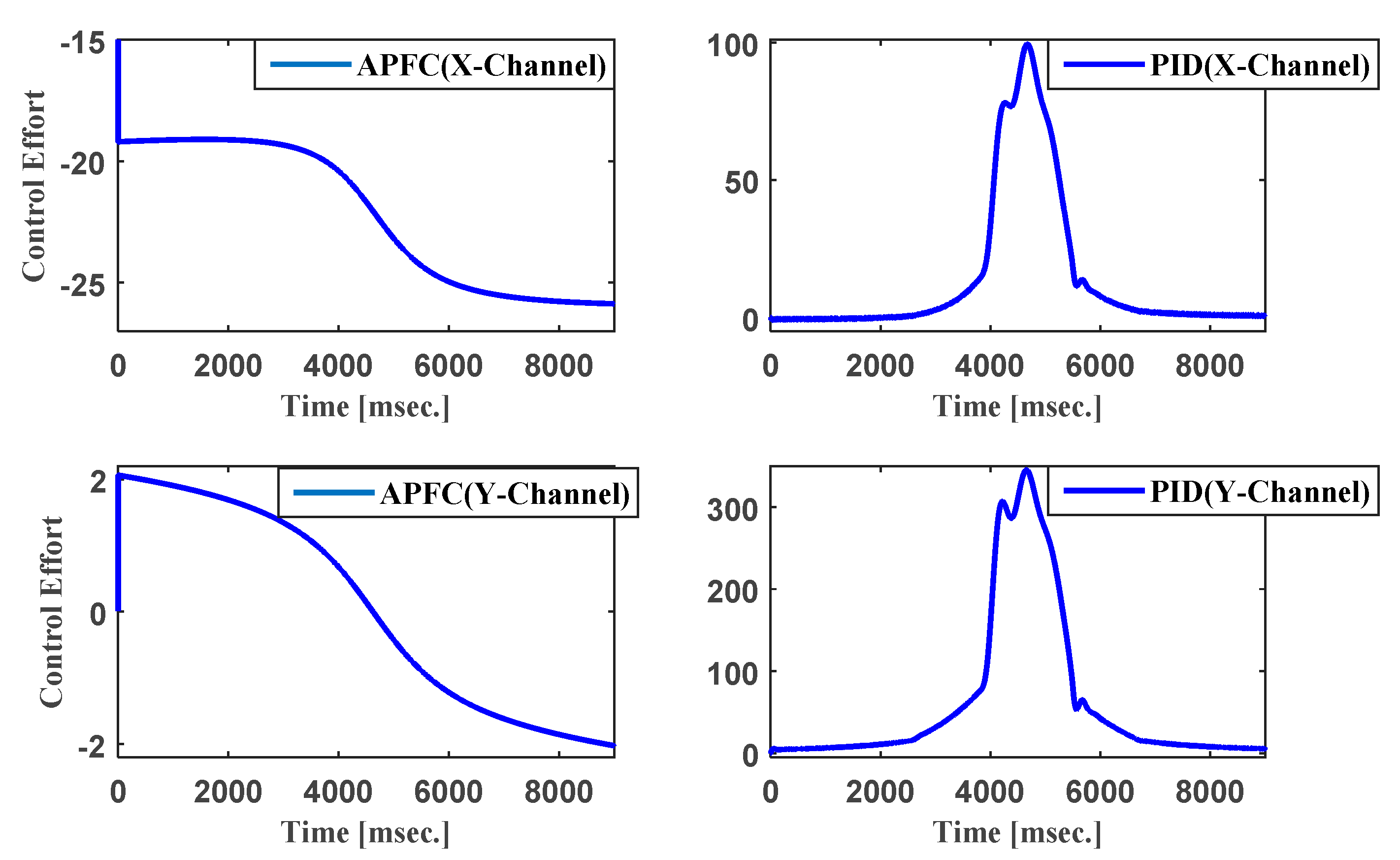
3. Results and Discussion

The control system is applied in the pedestal for tracking the satellite so that the antenna always faces the satellite. This ensures maximum energy absorption from the satellite signal. Hence, the satellite trajectory should be given to the system as the set point for the tracking process. This data in the form of elevation ($El$) and azimuth ($Az$) angles (which are calculated by NOAA software for P6 satellite, manufactured in India) is applied to the model. The P6 satellite trajectory, based on elevation and azimuth angles versus time, is illustrated in Figure 2 during one pass over the earth station. Using the mapping in (1), the satellite trajectory, in terms of ${\theta }_1$ and ${\theta }_2$, is shown in Figure 3, which is utilized as the reference input for tracking in the simulations of this section. The pedestal parameters are presented in

Table A1. Description of the parameters in Equation (2) and the values considered in the simulations.

Parameter	Description	Value	Dimension
${\mathrm{m}}_1$	mass of link-$1$	$250$	$kg$
${\mathrm{m}}_2$	mass of link-$2$	$250$	$kg$
$\mathrm{g}$	gravity acceleration	$9.8$	$m/s^2$
$\underset{{\mathrm{c}}_2}{\mathrm{x}}$	link-$2$ center of mass	$\left[-0.1775 0 0\right]$	$m$
$\underset{{\mathrm{xx}}_2}{\mathrm{I}}$	$\left(1,1\right)$th element of inertia matrix of link-$2$	$23.78$	$Kg.m^2$
$\underset{{\mathrm{yy}}_2}{\mathrm{I}}$	$\left(2,2\right)$th element of inertia matrix of link-$2$	$15.27$	$Kg.m^2$
$\underset{{\mathrm{zz}}_1}{\mathrm{I}}$	$\left(3,3\right)$th element of inertia matrix of link-$1$	$1$	$Kg.m^2$
$\underset{{\mathrm{zz}}_2}{\mathrm{I}}$	$\left(3,3\right)$th element of inertia matrix of link-$2$	$23.78$	$Kg.m^2$
${\mathrm{h}}_1$	length of link-$1$	$0.36$	$m$

. Two independent controllers are used for controlling the X and Y axes. The free parameters of APFC are selected as $\lambda =0.995,N=3,T=5,p=8,H_1=21,H_2=46$ for both axes. In addition, The PID coefficients for both axes are set as $K_P=50$, $K_I=20$, and $K_d=500$. The tuning of the PID coefficients is carried out by trial and error. However, $K_P$ and $K_I$ have been selected so as to achieve a short response time for the closed-loop system and to reduce the steady state tracking error as much as possible. It should be noted that the large value of $K_d$ in the PID controller results in the predictive behaviour of the controller. The reference input and the response of the closed-loop system with APFC and PID controllers are illustrated in Figure 4. According to the figure, it seems that both the PID and APFC controllers can track the satellite. For more clarity, the tracking errors for X and Y axes are shown in Figure 5. As seen, the tracking error is significantly smaller with the APFC in comparison to the PID controller and the closed-loop system with the APFC algorithm based on Laguerre functions is capable of tracking the desirable trajectory more accurately. This occurs to a greater extent during the moments when the satellite trajectory passes the degree of zero along the $Y$ axis.

The control efforts of the APFC and PID controllers are illustrated in Figure 6. It is obvious that the ranges of the control efforts for APFC and PID controllers are significantly different. An interesting feature of APFC is its desirable performance against the interference effects of the two channels. This is due the consideration of these effects in the system identification at every moment, which affects the system model in the next moment. If the satellite trajectory approaches zero along the Y axis (this occurs when the satellite is located in horizon), maximum acceleration is achieved along the inferior axis of the pedestal. This case is the same as when passing a satellite over an El/Az pedestal (zenith pass). In other words, the singular point for the X-Y pedestal is zero degrees along the inferior axis, namely, the Y axis. Hence, the control effort generated by the PID controller is higher at the moment, corresponding to zero degrees. However, in comparison to the APFC, the tracking error for the PID controller is significantly larger. On the other hand, the interference effect for the $X$ and $Y$ channels at these moments (corresponding to near zero degrees) is higher. Generally, the control effort generated by the PID controller is greater than that of the APFC, which may result in the saturation of actuators in the control system.

4. Conclusions

Due to the multivariable and nonlinear nature and the presence of time-varying unknown parameters in the X-Y pedestals, using adaptive control schemes is essential to controlling the X-Y pedestals in earth stations for LEO satellite tracking. Hence, this paper proposed an adaptive predictive functional control approach based on unstructured system identification. In the proposed algorithm, Laguerre functions are utilized for system modeling, while PFC is the control law. The results of applying this method to the X-Y pedestal for LEO satellite tracking were compared with the case of using the classic PID controller. Simulation results confirmed that, in comparison with the PID controller, the proposed algorithm achieves a higher accuracy, better control performance, reduction of X-Y pedestal tracking error in LEO satellite tracking, and requires less control effort. One of the main advantages of the proposed adaptive control scheme is its desirable performance against the interference effects of X and Y channels. This feature is obtained by the consideration of these effects in the system identification at every moment, which affects the system model in the next moment.

References

1. Tavassoli Hozouri, B. Eliminating Keyhole Problems in an X–Y Gimbal Assembly. U.S. Patent Application No. 11/405,892, 2007. Wo/2007/121393. Available online: https://patentimages.storage.googleapis.com/7a/9d/b7/07b45dcc3309d5/US20070241244A1.pdf (accessed on 30 August 2021).
2. Taheri, A.; Shoorehdeli, M.A.; Bahrami, H.; Fatehi, M.H. Implementation and control of X–Y pedestal using dual-drive technique and feedback error learning for LEO satellite tracking. IEEE Trans. Control Syst. Technol. 2014, 22, 1646–1657. [Google Scholar]
3. Looney, C.H.; Carlson, D.J.G. Coverage Diagrams for X–Y and Elevation-Over-Azimuth Antenna Mounts; Tech. Report No.: NASA-TN-D-2963; NASA Goddard Space Flight Center: Greenbelt, MD, USA, 1965.
4. Rolinski, A.J.; Carlson, D.J.; Coates, R.J. Satellite-Tracking Characteristics of the X–Y Mount for Data Acquisition Antennas; Tech. Report No.: NASA TN D-1697; NASA Goddard Space Flight Center: Greenbelt, MD, USA, 1964.
5. Rolinski, A.J.; Carlson, D.J.; Coates, R.J. The X–Y antenna mount for data acquisition from satellites. IRE Trans. Space Electron. Telemetry 1962, SET-8 (2), 159–163. [Google Scholar] [CrossRef]
6. Reisenfeld, S.; Aboutanios, E.; Willey, K.; Eckert, M.; Clout, R.; Thoms, A. The Design of the FedSat Ka Fast Tracking Earth Stations; Univ. Technol; Cooperative Research Centre for Satellite Systems Faculty of Engineering: Atlanta, GA, USA, 2008. [Google Scholar]
7. Tehrani, N.M.; Javanfar, E.; Vali, A.; Tehrani, H.M. Full extracting kinematic and dynamic equations of X/Y pedestal with velocity analysis. Proc. Int. Conf. Autom. Control 2014, 215–221. [Google Scholar] [CrossRef]
8. Aström, K.J.; Hagglund, T.; Hang, C.C.; Ho, W.K. Automatic tuning and adaptation for PID controllers-a survey. Control Eng. Pract. 1993, 1, 699–714. [Google Scholar] [CrossRef]
9. Zhang, R.; Xue, A.; Gao, F. PID Control Using Extended Non-Minimal State Space Model Optimization; Model Predictive Control; Springer: Singapore, 2019. [Google Scholar]
10. Wang, L. PID Control System Design and Automatic Tuning Using Matlab/Simulink; Wiley-IEEE Press: Hoboken, NJ, USA, 2020. [Google Scholar]
11. Huang, C.-N.; Chung, A. An intelligent design for a PID controller for nonlinear systems. Asian J. Control 2016, 18, 447–455. [Google Scholar] [CrossRef]
12. Ghahramani, A.; Karbasi, T.; Nasirian, M.; Sedigh, A.K. Predictive control of a two degrees of freedom XY robot (satellite tracking pedestal) and comparing GPC and GIPC algorithms for satellite tracking. In Proceedings of the 2nd International Conference on Control, Instrumentation and Automation, Shiraz, Iran, 27–29 December 2011; pp. 865–870. [Google Scholar]
13. Ghahramani, A.; Karbasi, T.; Nasirian, M.; Sedigh, A.K. Predictive control of earth station antenna (XY pedestal). In Proceedings of the 2nd International Conference on Control, Instrumentation and Automation, Shiraz, Iran, 27–29 December 2011; pp. 344–349. [Google Scholar]
14. Wang, H.; Zhao, X.; Tian, Y. Trajectory tracking control of XY table using sliding mode adaptive control based on fast double power reaching law. Asian J. Control 2016, 18, 2263–2271. [Google Scholar] [CrossRef]
15. Camacho, E.F.; Bordons, C. Model Predictive Control, 2nd ed.; Springer: London, UK, 2007. [Google Scholar]
16. Rossiter, J.A. Model-Based Predictive Control: A Practical Approach; CRC Press: Boca Raton, FL, USA, 2003. [Google Scholar]
17. Paulson, J.A.; Buehler, E.A.; Braatz, R.D.; Mesbah, A. Stochastic model predictive control with joint chance constraints. Int. J. Control 2020, 93, 126–139. [Google Scholar] [CrossRef]
18. Zhang, Z.; Rossiter, J.A.; Xie, L.; Su, H. Predictive functional control for integrator systems. J. Frankl. Inst. 2020, 357, 4171–4186. [Google Scholar] [CrossRef]
19. Wu, S.; Hou, P.; Zou, H. An improved constrained predictive functional control for industrial processes: A chamber pressure process study. Meas. Control 2020, 53, 833–840. [Google Scholar] [CrossRef]
20. Ridong, Z.; Anke, X.; Furong, G. Model Predictive Control: Approaches Based on the Extended State Space Model and Extended Non-minimal State Space Mode; Springer: Singapore, 2019. [Google Scholar]
21. Satoh, T.; Saito, N.; Nagase, J.-Y.; Saga, N. Predictive functional control of an axis positioning system with an estimator-based internal model. Control Eng. Pract. 2019, 86, 1–10. [Google Scholar] [CrossRef]
22. Richalet, J.; O’Donovan, D. Predictive Functional Control Principles and Industrial Applications; Springer: London, UK, 2009. [Google Scholar]
23. Astrom, K.J.; Wittenmark, B. Adaptive Control, 2nd ed.; Dover Publication: New York, NY, USA, 2008. [Google Scholar]
24. Wang, L.P. Discrete model predictive controller design using Laguerre functions. J. Process Contr. 2004, 14, 131–142. [Google Scholar] [CrossRef]
25. Zhang, H.; Chen, Z.; Wang, Y.; Li, M.; Qin, T. Adaptive predictive control algorithm based on Laguerre functional model. Int. J. Adapt. Control Signal Process. 2006, 20, 53–76. [Google Scholar] [CrossRef]
26. Hidayat, E.; Medvedev, A. Laguerre domain identification of continuous linear time-delay systems from impulse response data. Automatica 2012, 48, 2902–2907. [Google Scholar] [CrossRef]
27. Xu, M.; Li, X.; Liu, H.; Hao, Y. Adaptive predictive functional control with stochastic search. Proc. IEEE Int. Conf. Inform. Acquisition 2006, 1354–1358. [Google Scholar] [CrossRef]
28. Xu, M.; Liu, H.; Li, X.; Li, S. A steady adaptive predictive functional control with chaotic optimization. Proc. Sixth Int. Conf. Intell. Syst. Design Appl. 2006, 2, 137–141. [Google Scholar]
29. Ridong, Z.; Shuqing, W. Predictive functional controller with a similar proportional integral optimal regulator structure: Comparison with traditional predictive functional controller and application to heavy oil coking equipment. Chin. J. Chem. Eng. 2007, 15, 247–253. [Google Scholar]
30. Dadkhah Tehrani, R.; Ferdowsi, M.H. Adaptive predictive functional control with similar PI structure using unstructured system identification based on Laguerre functions. Int. J. Control Theory Comput. Model 2012, 2, 1–13. [Google Scholar] [CrossRef]
31. Plewa, P. Hardy’s inequality for Laguerre expansions of Hermite type. J. Fourier Anal. Appl. 2019, 25, 1855–1873. [Google Scholar] [CrossRef] [Green Version]
32. Rossiter, J.A.; Aftab, M.S. A Comparison of Tuning Methods for Predictive Functional Control. Processes 2021, 9, 1140. [Google Scholar] [CrossRef]
33. Rossiter, J.A.; Abdullah, M. Using Laguerre functions to improve the tuning and performance of predictive functional control. Int. J. Control 2021, 94, 202–214. [Google Scholar] [CrossRef] [Green Version]
34. Ljung, L. System Identification Theory for the User, 2nd ed.; Prentice-Hall: Upper Saddle River, NJ, USA, 1999. [Google Scholar]
35. Zhou, H.; Ma, G.; Yan, G.; Sun, X. Incremental recursive least-squares identification for the systems under poor observation condition. In Proceedings of the 2019 Chinese Control and Decision Conference (CCDC), Nanchang, China, 3–5 June 2019; pp. 1649–1652. [Google Scholar]
Figure 1. Satellite El/Az angles in earth station.
Applsci 11 09794 g001
Figure 2. Satellite trajectory presented in the form of elevation (El) and azimuth (Az) angles as the reference inputs.
Applsci 11 09794 g002
Figure 3. Satellite trajectory in terms of θ1 and θ2 as the reference inputs.
Applsci 11 09794 g003
Figure 4. The reference input, the response of the closed–loop control system using APFC scheme and PID controller for X and Y axes.
Applsci 11 09794 g004
Figure 5. Tracking error of X-Y pedestal system in X and Y axes for APFC scheme and PID controller.
Applsci 11 09794 g005
Figure 6. Control efforts generated by APFC scheme and PID controller.
Applsci 11 09794 g006
Publisher’s Note: MDPI stays neutral with regard to jurisdictional claims in published maps and institutional affiliations.