Axial-Symmetric Diffraction Radiation Antenna with a Very Narrow Funnel-Shaped Directional Diagram

Abstract

The paper is focused on reliable modeling and analysis of axially symmetric radiators with a very narrow (throat) funnel-shaped radiation pattern. When such a diagram is formed, a wave analogue of Smith–Purcell coherent radiation is realized—the surface wave of a radial dielectric waveguide ‘sweeps out’ with its exponentially decaying part a concentric periodic grating, the fundamental spatial harmonic of which, propagating without attenuation in a direction close to the symmetry axis of the structure, generates a radiation field with the required characteristics.

1. Introduction

A plane, density-modulated electron beam flying at a constant speed over a one-dimensional periodic grating generates in the surrounding space uniform plane electromagnetic waves; their number, the length, and direction of propagation are determined by the flow’s velocity and modulation period, as well as by the length of the grating’s period. This is a ‘coherent’ Smith–Purcell radiation (SPR) [1,2,3]. The same flow, passing at a constant speed in a medium, where the speed of light is less than its speed, generates there two homogeneous plane electromagnetic waves, diverging in a wedge from the direction of movement of the flow. The length of these waves and the direction of their propagation are determined by the period of modulation of the flow, the ratio of its speed to the speed of light in the medium, and by the sign of the refractive index of the medium. This is ‘coherent’ Vavilov–Cherenkov radiation (VChR) [4,5,6]. In this electromagnetic scenario, the field of the flow of charged particles generates the field of plane waves, above or below the grating, or in a sufficiently optically dense medium. We observe the same type of radiation and with the same characteristics in the case when we replace the electron flow with an open guiding structure (dielectric waveguide, for example), which supports the propagation of its eigen surface wave with phase velocity coinciding with the electron flow velocity. Here, we have the implementation of wave analogs of SPR and VChR. The analogy here is almost complete, since the field of the electron density-modulated flow is practically identical to the field of the eigen surface wave of the open guide line. The differences may be in the polarization of the fields, but they cannot change the picture of what is happening.

In diffraction radiation antennas (or simply in diffraction antennas) [7,8,9,10,11,12,13,14,15,16,17,18,19,20,21,22,23,24], wave analogs of SPR and VChR are implemented. It is impossible to say that they were very widespread, but several dozen devices of this type, unique in their characteristics, have been constructed at O.Ya. Usikov’s Institute for Radiophysics and Electronics of the Academy of Sciences of Ukraine (Kharkiv) for radar and radiometric systems of various purposes. These devices enabled the discovery of the solution to several urgent and practically important problems of remote sensing of the Earth using aerospace carriers, problems of monitoring the airfield and protecting the perimeters of airports, problems of preventing collisions in automobile, river, and sea transport, problems of ‘blind’ landing of helicopters, and problems of short-range radar and radiometry.

The problems that have to be solved for creating efficiently operating diffraction radiation antennas are essentially the same as in the case of phased antenna arrays—it is necessary to ensure, first of all, the required amplitude–phase distribution of the field at sufficiently large (in relation to the size of the period of the used gratings) apertures. These problems have to be solved in different ways: in antenna arrays, each elementary emitter (usually, it is associated with one period of the grating) is excited according to a certain program, and in diffraction, antennas all such emitters are excited by the field of surface wave of an open guiding line; it is necessary to ensure that the phase velocity of this wave is not distorted, and that the amplitude decreases meet the required amplitude distribution of the field at the aperture. The costs of these solutions’ implementation differ significantly—with diffraction antennas, they are much lower.

In operating systems, mainly linear [7,9,12,16,18,19,20,21,22] and planar [7,10,11,13,14,15,16,17,24] antennas of diffraction radiation were used. In the radiator of a linear antenna, the grating width and the effective width of the open (dielectric) waveguide are from half to two wavelengths, and the length of the radiating aperture is from several tens to several hundred wavelengths. In planar antennas allowing electromechanical beam scanning in two planes, the effective width of the grating and the effective width of the open (dielectric) waveguide, as well as the length of the emitting aperture, are measured in tens and hundreds of wavelengths.

Axially symmetric emitters based on circular dielectric waveguides and Goubau lines have been studied well enough theoretically [17,22,25], but they were implemented only in laboratory models and in prototypes with short apertures—they were used to solve the problems of synthesizing antennas with full-size apertures. The axially symmetric structure considered in this work implements a wave analogue of Smith–Purcell radiation in the ‘radial dielectric waveguide—concentric periodic grating’ system and is capable, due to the specific geometry of such a system, to form a radiation field with a very narrow funnel-shaped directivity pattern near the throat. Antennas with such patterns are in demand when solving several specific radar problems.

We construct a numerical solution of model problems, providing simulation and analysis of all physical features of the processes of electromagnetic waves transformation in the structures under consideration, applying the method of exact absorbing conditions [25,26,27,28,29,30,31,32,33,34,35,36]. The results of works [31,36,37] convincingly testify to its reliability and efficiency.

We use SI, the International System of Units, for all physical parameters except the ‘time’ $t$, which is the product of the natural time and the velocity of light in vacuum; thus, $t$ is measured in meters. In this paper, all dimensions are omitted. According to SI, all geometrical parameters ($a, b, c$, etc.) are given in meters. However, this is obviously not a serious obstacle to extend the results to any other geometrically similar structure.

2. Models of the Method of Exact Absorbing Conditions Time Domain Representations

Axially symmetric emitters, excited by eigen $T{E}_{0p}$- or $T{M}_{0p}$- pulse wave $V_p\left(g,t\right)=v_p\left(z,t\right){\mu }_p^{+}\left(\rho \right)$, $g=\left\{\rho ,z\right\}\in \mathrm{A}$ of circular or coaxial waveguide $\mathrm{A}$, coming on the virtual boundary ${\mathrm{L}}^{+}$ (see Figure 1: the structures are homogeneous along the axis $\varphi$) at time moments $t>0$, are studied by solving the following model problem of the method of exact absorbing conditions [25,32,34]:

$$\{\begin{array}{l}\left[-\epsilon \left(g\right){\partial }_t^2-\sigma \left(g\right){\eta }_0{\partial }_t+{\partial }_{\rho }\left({\rho }^{-1}{\partial }_{\rho }\rho \right)+{\partial }_z^2\right]U\left(g,t\right)=0; g=\left\{\rho ,z\right\}\in {\mathsf{\Omega }}_{\mathrm{int}}, t>0\\ U\left(g,0\right)=0, {{\partial }_{t}U\left(g,t\right)|}_{t=0}=0; g\in \overline{{\mathsf{\Omega }}_{\mathrm{int}}}\\ {\mathbf{E}}_{\mathrm{tg}}\left(q,t\right) \mathrm{and} {\mathbf{H}}_{\mathrm{tg}}\left(q,t\right), q=\left\{\rho ,\varphi ,z\right\} \mathrm{are} \mathrm{continuous} \mathrm{when} \mathrm{crossing} {\mathsf{\Sigma }}^{\epsilon ,\sigma },\\ {{\mathbf{E}}_{\mathrm{tg}}\left(q,t\right)|}_{q\in \mathsf{\Sigma }}=0, U\left(0,z,t\right)=0 \mathrm{for} \left\{0,z\right\}\in \overline{{\mathsf{\Omega }}_{\mathrm{int}}} \mathrm{and} {D^{-}\left[U\left(g,t\right)\right]|}_{g\in {\mathrm{L}}^{-}}=0,\\ {D^{+}\left[U\left(g,t\right)-V_p\left(g,t\right)\right]|}_{g\in {\mathrm{L}}^{+}}=0, {D\left[U\left(g,t\right)\right]|}_{g\in \mathrm{L}}=0; t\ge 0.\end{array}$$

(1)

Here, $V_p\left(g,t\right)$ is the $E_{\varphi }$- or $H_{\varphi }$- field component of the exciting $T{E}_{0p}$- or $T{M}_{0p}$- pulse waveguide wave; $v_p\left(z,t\right)$ and ${\mu }_p^{+}\left(\rho \right)$ are its space–time amplitude and transverse eigen function respectively; $\overline{\mathrm{G}}$ is the closure of $\mathrm{G}$; $U\left(g,t\right)=E_{\varphi }\left(g,t\right)$ in the case of $T{E}_0$-waves ($E_{\rho }=E_z=H_{\varphi }\equiv 0$, ${\partial }_{\varphi }=0$) and $U\left(g,t\right)=H_{\varphi }\left(g,t\right)$ for $T{M}_0$-waves ($H_{\rho }=H_z=E_{\varphi }\equiv 0$, ${\partial }_{\varphi }=0$); $\mathbf{E}\left(q,t\right)=\left\{E_{\rho },E_{\varphi },E_z\right\}$ and $\mathbf{H}\left(q,t\right)=\left\{H_{\rho },H_{\varphi },H_z\right\}$ are the vectors of the electric and magnetic fields, respectively; $\left\{\rho ,\varphi ,z\right\}$ and $\left\{r,\vartheta ,\varphi \right\}$ are the cylindrical and spherical coordinates, respectively; piecewise constant functions $\sigma \left(g\right)\ge 0$ and $\epsilon \left(g\right)>0$ specify a conductivity and relative permittivity of non-magnetic elements of the structure; ${\eta }_0={\left({\mu }_0/{\epsilon }_0\right)}^{1/2}$ is an impedance of free space; ${\epsilon }_0$ and ${\mu }_0$ are electric and magnetic vacuum constants, respectively. The surfaces $\mathsf{\Sigma }={\mathsf{\Sigma }}_{\varphi }\times \left[0\le \varphi \le 2\pi \right]$ of perfectly conducting elements of the structure and surfaces ${\mathsf{\Sigma }}^{\epsilon ,\sigma }={\mathsf{\Sigma }}_{\varphi }^{\epsilon ,\sigma }\times \left[0\le \varphi \le 2\pi \right]$, where the constitutive parameters $\sigma \left(g\right)$ and $\epsilon \left(g\right)$ are discontinuous, are assumed to be sufficiently smooth. Nonzero components of the electromagnetic field lying in the half-plane ${\mathsf{\Omega }}_{\mathrm{total}}=\left\{q=\left\{\rho ,\varphi ,z\right\}: \rho >0, \left|z\right|\ge 0, \varphi =const\right\}$ are determined by the expressions

$${\partial }_t{H}_{\rho }\left(g,t\right)={\eta }_0^{-1}{\partial }_z{E}_{\varphi }\left(g,t\right), {\partial }_t{H}_z\left(g,t\right)=-{\eta }_0^{-1}{\rho }^{-1}{\partial }_{\rho }\left[\rho E_{\varphi }\left(g,t\right)\right]$$

(2)

in the case of $T{E}_0$-waves, and in the case of $T{M}_0$-waves, by relations

$$\begin{array}{l}\left[\epsilon \left(g\right){\eta }_0^{-1}{\partial }_t+\sigma \left(g\right)\right]E_{\rho }\left(g,t\right)=-{\partial }_z{H}_{\varphi }\left(g,t\right),\\ \left[\epsilon \left(g\right){\eta }_0^{-1}{\partial }_t+\sigma \left(g\right)\right]E_z\left(g,t\right)={\rho }^{-1}{\partial }_{\rho }\left[\rho H_{\varphi }\left(g,t\right)\right].\end{array}$$

(3)

Computational domain ${\mathsf{\Omega }}_{\mathrm{int}}$ of the problem (1) is a part of the plane ${\mathsf{\Omega }}_{\mathrm{total}}$, limited by contour ${\mathsf{\Sigma }}_{\varphi }^{\epsilon ,\sigma }$, axis $z$, virtual boundaries ${\mathrm{L}}^{\pm }$ (input and output ports in the cross section of virtual waveguides $\mathrm{A}$ and $\mathrm{B}$) and by a ‘spherical’ boundary $\mathrm{L}=\left\{g=\left\{r,\vartheta \right\}: r=L\right\}$, separating ${\mathsf{\Omega }}_{\mathrm{int}}$ from free space ${\mathsf{\Omega }}_{\mathrm{ext}}=\left\{g=\left\{r,\vartheta \right\}: r>L\right\}$ in ${\mathsf{\Omega }}_{\mathrm{total}}$. The arc $\mathrm{L}$ of radius $L$ covers all scattering inhomogeneities of the domain ${\mathsf{\Omega }}_{\mathrm{int}}$.

Exact absorbing conditions ${D^{+}\left[U\left(g,t\right)-V_p\left(g,t\right)\right]|}_{g\in {\mathrm{L}}^{+}}=0$, ${D^{-}\left[U\left(g,t\right)\right]|}_{g\in {\mathrm{L}}^{-}}=0$ and ${D\left[U\left(g,t\right)\right]|}_{g\in \mathrm{L}}=0$ for virtual boundaries are the ideal model for waves

$$\begin{array}{l}U\left(g,t\right)-V_p\left(g,t\right)=U^{+}\left(g,t\right)={\displaystyle \sum _{n\in \left\{n\right\}}{U}_{np}^{+}\left(g,t\right)}={\displaystyle \sum _{n\in \left\{n\right\}}{u}_{np}^{+}\left(z,t\right){\mu }_n^{+}\left(\rho \right)}; g\in \overline{\mathrm{A}}, t\ge 0,\\ U\left(g,t\right)=U^{-}\left(g,t\right)={\displaystyle \sum _{n\in \left\{n\right\}}{U}_{np}^{-}\left(g,t\right)}={\displaystyle \sum _{n\in \left\{n\right\}}{u}_{np}^{-}\left(z,t\right){\mu }_n^{-}\left(\rho \right)}; g\in \overline{\mathrm{B}}, t\ge 0, \mathrm{and}\\ U\left(g,t\right)={\displaystyle \sum _{m=1}^{\infty }{U}_{mp}\left(g,t\right)}={\displaystyle \sum _{m=1}^{\infty }{u}_{mp}\left(r,t\right)}{\overline{\mu }}_m\left(\vartheta \right); r\ge L, 0\le \vartheta \le \pi , t\ge 0,\end{array}$$

(4)

traveling from domain ${\mathsf{\Omega }}_{\mathrm{int}}$ into waveguides $\mathrm{A}$, $\mathrm{B}$, and domain ${\mathsf{\Omega }}_{\mathrm{ext}}$ [25,32,34]. Here, $\left\{n\right\}=0,1,2,\dots$ only in the case of coaxial waveguides and only for $T{M}_0$-waves; in all other cases $\left\{n\right\}=1,2,3,\dots$.

Explicit analytic representations for transverse functions ${\mu }_n^{\pm }\left(\rho \right)$ and the corresponding eigen values ${\lambda }_n^{\pm }$ are well known [25,31,32,34]. For example, for $T{E}_0$-waves functions ${\mu }_n^{\pm }\left(\rho \right)$ of coaxial waveguide ($b$ is the radius of its inner conductor, $a$ is the radius of its outer conductor) have a form

$$\{\begin{array}{l}{\mu }_n\left(\rho \right)=G_1\left({\lambda }_n,\rho \right)\sqrt{2}{\left[a^2{G}_0^2\left({\lambda }_n,a\right)-b^2{G}_0^2\left({\lambda }_n,b\right)\right]}^{-1/2}; b<\rho <a\\ {\lambda }_n>0 \mathrm{are} \mathrm{the} \mathrm{roots} \mathrm{of} \mathrm{the} \mathrm{equation} G_1\left(\lambda ,a\right)=0;\\ G_q\left(\lambda ,\rho \right)=J_q\left(\lambda \rho \right)N_1\left(\lambda b\right)-N_q\left(\lambda \rho \right)J_1\left(\lambda b\right); q=0,1\end{array}$$

(5)

and

$$\{\begin{array}{l}{\mu }_n\left(\rho \right)=J_1\left({\lambda }_n\rho \right)\sqrt{2}{\left[a{J}_0\left({\lambda }_{n}a\right)\right]}^{-1}; 0<\rho <a\\ {\lambda }_n>0 \mathrm{are} \mathrm{the} \mathrm{roots} \mathrm{of} \mathrm{the} \mathrm{equation} J_1\left(\lambda a\right)=0\end{array}$$

(6)

for a circular waveguide. Here, $J_q\left(\dots \right)$ и $N_q\left(\dots \right)$ are cylindrical Bessel and Neumann functions.

The transverse functions

$${\overline{\mu }}_m\left(\vartheta \right)={\tilde{\mu }}_m\left(\cos \vartheta \right)=\sqrt{\left(2m+1\right)/\left(2m\left(m+1\right)\right)} P_m^1\left(\cos \vartheta \right),$$

(7)

($P_m^1\left(\dots \right)$ are associated Legendre functions) have relevant eigen values ${\overline{\lambda }}_m=\sqrt{m\left(m+1\right)}$, $m=1,2,3,\dots$ [32,34].

The works [25,26,27,28,29,30,31,32,33,34,35,36,37] are devoted to the theory and construction of exact absorbing conditions for open initial-boundary value problems in computational electrodynamics. It is possible to find there, in particular, such analytical representations for integro-differential operators $D^{\pm }\left[\dots \right]$ and $D\left[\dots \right]$ of the problem (1) (presume—see Figure 1—that virtual boundaries ${\mathrm{L}}^{\pm }$ lie in the plane $z=0$):

$$\begin{array}{l}U\left(\rho ,0,t\right)-V_p\left(\rho ,0,t\right)={\displaystyle \sum _{n\in \left\{n\right\}}\{{\displaystyle \underset{0}{\overset{t}{\int }}{J}_0\left[{\lambda }_n^{+}\left(t-\tau \right)\right]}}\times \\ \times \left[{\displaystyle \underset{b}{\overset{a}{\int }}{{\partial }_z\left[U\left(\tilde{\rho },z,\tau \right)-V_p\left(\tilde{\rho },z,\tau \right)\right]|}_{z=0}}{\mu }_n^{+}\left(\tilde{\rho }\right)\tilde{\rho } d\tilde{\rho }\right]d\tau \}\times \\ \times {\mu }_n^{+}\left(\rho \right); 0\le b\le \rho \le a, t\ge 0,\end{array}$$

(8)

$$\begin{array}{l}U\left(\rho ,0,t\right)=-{\displaystyle \sum _{n\in \left\{n\right\}}\left\{{\displaystyle \underset{0}{\overset{t}{\int }}{J}_0\left[{\lambda }_n^{-}\left(t-\tau \right)\right]\left[{\displaystyle \underset{b}{\overset{a}{\int }}{{\partial }_{z}U\left(\tilde{\rho },z,\tau \right)|}_{z=0}}{\mu }_n^{-}\left(\tilde{\rho }\right)\tilde{\rho } d\tilde{\rho }\right]d\tau }\right\}}{\mu }_n^{-}\left(\rho \right);\\ 0<b\le \rho \le a, t\ge 0,\end{array}$$

(9)

$$\begin{array}{l}U\left(L,\vartheta ,t\right)={\displaystyle \sum _{m=1}^{\infty }\{{\displaystyle \underset{t-2L}{\overset{t}{\int }}[\left(\frac{{\left(t-\tau \right)}^2}{2L^3}{{\partial }_q{P}_m\left(q\right)|}_{q=1-\frac{{\left(t-\tau \right)}^2}{2L^2}}-\frac{1}{L}{P}_m\left(1-\frac{{\left(t-\tau \right)}^2}{2L^2}\right)\right)\times }}\\ \times {\displaystyle \underset{0}{\overset{\pi }{\int }}U\left(L,\tilde{\vartheta },\tau \right)}{\tilde{\mu }}_m\left(\cos \tilde{\vartheta }\right)\sin \tilde{\vartheta }d\tilde{\vartheta }-P_m\left(1-\frac{{\left(t-\tau \right)}^2}{2L^2}\right){\displaystyle \underset{0}{\overset{\pi }{\int }}{\partial }_{r}U\left(L,\tilde{\vartheta },\tau \right){\tilde{\mu }}_m\left(\cos \tilde{\vartheta }\right)\sin \tilde{\vartheta }d\tilde{\vartheta }}]d\tau +\\ +{\left(-1\right)}^m{\displaystyle \underset{0}{\overset{\pi }{\int }}U\left(L,\tilde{\vartheta },t-\left(r+L\right)\right) }{\tilde{\mu }}_m\left(\cos \tilde{\vartheta }\right)\sin \tilde{\vartheta }d\tilde{\vartheta }\}{\tilde{\mu }}_m\left(\cos \vartheta \right); 0\le \vartheta \le \pi , t>0\end{array}$$

(10)

($P_m\left(\dots \right)$ are Legendre polynomials).

Systems of transverse functions ${\left\{{\mu }_n^{\pm }\left(\rho \right)\right\}}_{n\in \left\{n\right\}}$ and ${\left\{{\overline{\mu }}_m\left(\vartheta \right)\right\}}_{m=1}^{\infty }$ are complete and orthonormal (with a certain weight) on the corresponding intervals of $\rho$ and $\vartheta$ variation. Spatial–temporal amplitudes $u_{np}^{\pm }\left(z,t\right)$, $u_{mp}\left(r,t\right)$ for the values $z$ and $r$, corresponding to the boundaries ${\mathrm{L}}^{\pm }$ and $\mathrm{L}$, are determined from the solution to the problem (1). Values of $u_{mp}\left(r,t\right)$, $r>L$, required for constructing the radiation pattern of the emitter, are obtained from $u_{mp}\left(L,t\right)$, using the so-called ‘transport operators’ [31,34,38,39,40]. Function $V_p\left(g,t\right)$ and its derivative with respect to $z$ on the boundary ${\mathrm{L}}^{+}$ must be given by their space–time amplitudes $v_p\left(0,t\right)$ and ${{\partial }_z{v}_p\left(z,t\right)|}_{z=0}$ in order to meet the condition (8). Making a choice for the values of the function $v_p\left(0,t\right)$ on a finite interval $0<T_1\le t\le T_2<T$ ($T$ is the upper limit of the observation time), we have no restrictions. This choice is imposed mainly by the specifics of the problem and the conditions of the computational experiment. However, the function ${{\partial }_z{v}_p\left(z,t\right)|}_{z=0}$ determining the normal derivative of the function $V_p\left(g,t\right)$ on ${\mathrm{L}}^{+}$ cannot be chosen arbitrarily. The causality principle requires the strict correspondence of a pair of functions

$$\left\{v_p\left(0,t\right){\mu }_p^{+}\left(\rho \right); \left[{{\partial }_z{v}_p\left(z,t\right)|}_{z=0}\right]{\mu }_p^{+}\left(\rho \right)\right\}$$

(11)

to eigen pulse wave ($T{E}_{0p}$- or $T{M}_{0p}$-), propagating along the waveguide $\mathrm{A}$ in the direction of increasing values of $z$. This requirement is fulfilled if the pair of functions (11) is connected by the relation

$$v_p\left(0,t\right)=-{\displaystyle \underset{0}{\overset{t}{\int }}{J}_0\left[{\lambda }_p^{+}\left(t-\tau \right)\right]}{{\partial }_z{v}_p\left(z,t\right)|}_{z=0}d\tau ; t\ge 0,$$

(12)

obtained in the same way as the exact absorbing conditions (8) and (9) [25,32,34].

3. Frequency Domain Representations

The solution $U\left(g,t\right)$ to the problem (1) and (4) (we construct it by implementing the standard computational schemes of the finite difference method [41]) and the solution $\tilde{U}\left(g,k\right)$ to the problem

$$\{\begin{array}{l}\left[{\partial }_z^2+{\partial }_{\rho }\left({\rho }^{-1}{\partial }_{\rho }\rho \right)+\overline{\epsilon }\left(g\right)k^2\right]\tilde{U}\left(g,k\right)=0; g=\left\{\rho ,z\right\}\in {\mathsf{\Omega }}_{\mathrm{int}}\\ {{\tilde{\mathbf{E}}}_{\mathrm{tg}}\left(q,k\right)|}_{q=\left\{\rho ,\varphi ,z\right\}\in \mathsf{\Sigma }}=0, \tilde{U}\left(0,z,k\right)=0 \mathrm{for} \left\{0,z\right\}\in \overline{{\mathsf{\Omega }}_{\mathrm{int}}}\\ {\tilde{\mathbf{E}}}_{\mathrm{tg}}\left(q,k\right), {\tilde{\mathbf{H}}}_{\mathrm{tg}}\left(q,k\right) \mathrm{are} \mathrm{continuous} \mathrm{when} \mathrm{crossing} {\mathsf{\Sigma }}^{\epsilon ,\sigma }\\ \mathrm{and} \mathrm{boundaries} \mathrm{L}\times \left[0,2\pi \right], {\mathrm{L}}^{\pm }\times \left[0,2\pi \right],\end{array}$$

(13a)

$$\begin{array}{l}\tilde{U}\left(g,k\right)={\tilde{V}}_p\left(g,k\right)+{\tilde{U}}^{+}\left(g,k\right)={\tilde{V}}_p\left(g,k\right)+{\displaystyle \sum _{n\in \left\{n\right\}}{\tilde{U}}_{np}^{+}\left(g,k\right)}=\\ =A_p\left(k\right)\exp \left(i{\gamma }_p^{+}z\right){\mu }_p^{+}\left(\rho \right)+{\displaystyle \sum _{n\in \left\{n\right\}}{B}_{np}^{+}\left(k\right)\exp \left(-i{\gamma }_n^{+}z\right)}{\mu }_n^{+}\left(\rho \right); g\in \overline{\mathrm{A}},\end{array}$$

(13b)

$$\tilde{U}\left(g,k\right)={\tilde{U}}^{-}\left(g,k\right)={\displaystyle \sum _{n\in \left\{n\right\}}{\tilde{U}}_{np}^{-}\left(g,k\right)}={\displaystyle \sum _{n\in \left\{n\right\}}{B}_{np}^{-}\left(k\right)\exp \left(-i{\gamma }_n^{-}z\right){\mu }_n^{-}\left(\rho \right)}; g\in \overline{\mathrm{B}},$$

(13c)

$$\tilde{U}\left(g,k\right)={\displaystyle \sum _{m=1}^{\infty }{\tilde{U}}_{mp}\left(g,k\right)}=\frac{1}{\sqrt{r}}{\displaystyle \sum _{m=1}^{\infty }{C}_{mp}\left(k\right)H_{m+1/2}^{\left(1\right)}\left(kr\right){\tilde{\mu }}_m\left(\cos \vartheta \right)}; g\in \overline{{\mathsf{\Omega }}_{\mathrm{ext}}},$$

(13d)

are connected by integral transformation $\tilde{f}\left(k\right)={\displaystyle {\int }_0^{\infty }f\left(t\right)\exp \left(ikt\right)dt}$ [25,32,34] (actually by integral transformation $\tilde{f}\left(k\right)={\displaystyle {\int }_0^{T}f\left(t\right)\exp \left(ikt\right)dt}$; $T<\infty$ is an observation time in computational experiments). This transformation matches the characteristics of the time domain $f\left(t\right)$ with the characteristics of the frequency domain $\tilde{f}\left(k\right)$—$\tilde{f}\left(k\right)\leftrightarrow f\left(t\right)$. Here, $H_{m+1/2}^{\left(1\right)}\left(\dots \right)$ are cylindrical Hankel functions, $\tilde{U}\left(g,k\right)={\tilde{E}}_{\varphi }\left(g,k\right)$ in the case of monochromatic $T{E}_0$-waves and $\tilde{U}\left(g,k\right)={\tilde{H}}_{\varphi }\left(g,k\right)$ in the case of monochromatic $T{M}_0$-waves; $k$ is a wavenumber (frequency parameter or just frequency, is related with frequency $f\left[Hz\right]$ by the ratio $f\left[Hz\right]=\frac{v\left[m/s\right]}{2\pi }k\left[rad/m\right]$, where $v\left[m/s\right]$ is a speed of light in vacuum), $\overline{\epsilon }\left(g\right)=\epsilon \left(g\right)+i{\eta }_0\sigma \left(g\right)/k$ and

$${\gamma }_n^{\pm }=\sqrt{k^2-{\left({\lambda }_n^{\pm }\right)}^2}; \mathrm{Re}{\gamma }_n^{\pm }\ge 0, \mathrm{Im}{\gamma }_n^{\pm }\ge 0$$

(14)

are longitudinal wavenumbers of $T{E}_{0n}$- or $T{M}_{0n}$- monochromatic eigen waves propagating in waveguides $\mathrm{A}$ and $\mathrm{B}$ with (if $\mathrm{Im}{\gamma }_n^{\pm }>0$) or without (if $\mathrm{Im}{\gamma }_n^{\pm }=0$) attenuation.

In Formula (13b,c), the term with the complex amplitude $A_p$ corresponds to the monochromatic wave ${\tilde{V}}_p\left(g,k\right) \leftrightarrow V_p\left(g,t\right)$ arriving at the boundary ${\mathrm{L}}^{+}$, and the terms with the amplitudes, $B_{np}^{+}$, $B_{np}^{-}$, and $C_{mp}$, to the waves of the secondary field ${\tilde{U}}_{np}^{+}\left(g,k\right) \leftrightarrow U_{np}^{+}\left(g,t\right)$, ${\tilde{U}}_{np}^{-}\left(g,k\right) \leftrightarrow U_{np}^{-}\left(g,t\right)$, and ${\tilde{U}}_{mp}\left(g,k\right)\leftrightarrow U_{mp}\left(g,t\right)$, both in the waveguides $\mathrm{A}$, $\mathrm{B}$ and in a free space. If we compare representations (13b–d) and (4), it becomes obvious that

$$A_p\left(k\right) \leftrightarrow v_p\left(0,t\right), B_{np}^{\pm }\left(k\right) \leftrightarrow u_{np}^{\pm }{}_{np}\left(0,t\right),$$

(15)

or, in another notation, $A_p\left(k\right) = {\tilde{v}}_p\left(0,k\right)$, $B_{np}^{\pm }\left(k\right) = {\tilde{u}}_{np}^{\pm }\left(0,k\right)$. Similarly, we obtain

$$\frac{C_{mp}\left(k\right)H_{m+1/2}^{\left(1\right)}\left(kr\right)}{\sqrt{r}} \leftrightarrow u_{mp}\left(r,t\right) \mathrm{or} \frac{C_{mp}\left(k\right)H_{m+1/2}^{\left(1\right)}\left(kr\right)}{\sqrt{r}}={\tilde{u}}_{mp}\left(r,k\right).$$

(16)

In the boundary value problem (13), expressions (13b–d) represent the so-called ‘partial radiation conditions’ [38], corresponding to the physically grounded requirement of the absence in the field $\tilde{U}\left(g,k\right)$ waves coming from infinity. An exception is possible only for the ‘incident’ wave. In our case, this wave is determined by the function

$${\tilde{V}}_p\left(g,k\right)=A_p\left(k\right)\exp \left(i{\gamma }_p^{+}z\right){\mu }_p^{+}\left(\rho \right); \mathrm{Im}{\gamma }_p^{+}=0, g\in \mathrm{A} ¯.$$

(17)

In the frequency domain, the structure under consideration is characterized (in part) by the reflection coefficients $R_{np}\left(k\right)$ (the conversion coefficients of the $p$-th incident from the waveguide $\mathrm{A}$ wave into $n$-th reflected wave) and the transmission coefficients $T_{np}\left(k\right)$ (the conversion coefficients of the $p$-th wave of the waveguide $\mathrm{A}$ into the $n$-th wave of the waveguide $\mathrm{B}$). These coefficients, given by $R_{np}\left(k\right)=B_{np}^{+}/A_p$, $T_{np}\left(k\right)=B_{np}^{-}/A_p$, and values

$$W_{\mathrm{abs}}\left(k\right)=\frac{k^2}{{\gamma }_p^{+}\beta }{{\displaystyle \underset{{\mathsf{\Omega }}_{\mathrm{int}}}{\int }\mathrm{Im}\overline{\epsilon }\left(g\right)\left|\tilde{\mathbf{E}}\left(g,k\right)\right|}}^{2}dg, W_{np}^{+}\left(k\right)={\left|R_{np}\right|}^2\frac{\mathrm{Re}{\gamma }_n^{+}}{{\gamma }_p^{+}}, W_{np}^{-}\left(k\right)={\left|T_{np}\right|}^2\frac{\mathrm{Re}{\gamma }_n^{-}}{{\gamma }_p^{+}}$$

(18)

($\beta =1$ for $T{E}_0$-waves, and $\beta ={\eta }_0^2$ for $T{M}_0$-waves, $dg=\rho d\rho dz$) determine [34] the relative fraction of the energy absorbed in non-ideal elements of the structure and directed to each of the waves propagating in the waveguides $\mathrm{A}$ and $\mathrm{B}$. For any finite value $k=2\pi /\lambda$ ($\lambda$ is the wavelength in free space), the number $N^{+}+N^{-}$, $N^{\pm }={\displaystyle {\sum }_n\left(\mathrm{Re}{\gamma }_n^{\pm }/\left|{\gamma }_n^{\pm }\right|\right)}$ of such waves taking away the energy supplied to the axially symmetric structure is finite. It follows from (18) that the fraction of the energy emitted by the structure into free space through the virtual boundary $\mathrm{L}$ (radiation efficiency) can be calculated by the formula

$$\eta \left(k\right)=1-W_{\mathrm{abs}}\left(k\right)-{\displaystyle \sum _n\left(W_{np}^{+}\left(k\right)+W_{np}^{-}\left(k\right)\right)}.$$

(19)

Normalized radiation pattern on the arc $r=M\ge L$

$$D\left(\vartheta ,k,M\right)=\frac{{\left|{\tilde{\mathbf{E}}}_{\mathrm{tg}}\left(M,\vartheta ,k\right)\right|}^2}{\underset{0\le \tilde{\vartheta }\le \pi }{\max }{\left|{\tilde{\mathbf{E}}}_{\mathrm{tg}}\left(M,\tilde{\vartheta },k\right)\right|}^2}; 0\le \vartheta \le {180}^{\circ }, K_1\le k\le K_2$$

(20)

determines the spatial orientation and ‘energy capacity’ of waves radiated into free space. Here, ${\tilde{\mathbf{E}}}_{\mathrm{tg}}\left(M,\vartheta ,k\right)$ is a tangential (with respect to the spherical surface $r=M$) component of the monochromatic electric field $\tilde{\mathbf{E}}\left(q,k\right)$. The value $M$ determines the zone (near, mid, far) where the diagram $D\left(\vartheta ,k,M\right)$ is calculated. We presume that the boundary of the near zone is given by equality $M=L$, and the far zone is determined by such values of $M$, further increase in which does not lead to significant changes in the function for all considered values $k$.

The main lobe of the radiation pattern is directed at an angle $\overline{\vartheta }\left(k\right)$ such that $D\left(\overline{\vartheta }\left(k\right),k,M\right)=1$. The width of the main lobe ${\vartheta }_{0.5}\left(k\right)$ is defined as the angle between two (${\vartheta }^{+}$ and ${\vartheta }^{-}$) directions in the main lobe of the diagram for which the radiated power is halved in relation to the maximum, i.e., ${\vartheta }_{0.5}\left(k\right)=\left|{\vartheta }^{+}-{\vartheta }^{-}\right|$, where $D\left({\vartheta }^{+},k,M\right)=0.5$ and $D\left({\vartheta }^{-},k,M\right)=0.5$.

For calculating the radiation pattern $D\left(\vartheta ,k,M\right)$, it is necessary to solve the initial boundary value problem (1), and then, using the exact radiation condition [25,32,34], from which absorbing condition (10) follows, to determine, by the values of $U\left(g,t\right)$ on the arc $r=L$, the values of $U\left(g,t\right)$ and ${\mathbf{E}}_{\mathrm{tg}}\left(M,\vartheta ,t\right)$ ($E_{\varphi }\left(M,\vartheta ,t\right)$ for $T{E}_0$-waves or $E_{\vartheta }\left(M,\vartheta ,t\right)$ for $T{M}_0$-waves (see formulas (1.19) in [31]) on the arc $r=M$, and, finally, to use the transformation $\tilde{f}\left(k\right)\leftrightarrow f\left(t\right)$.

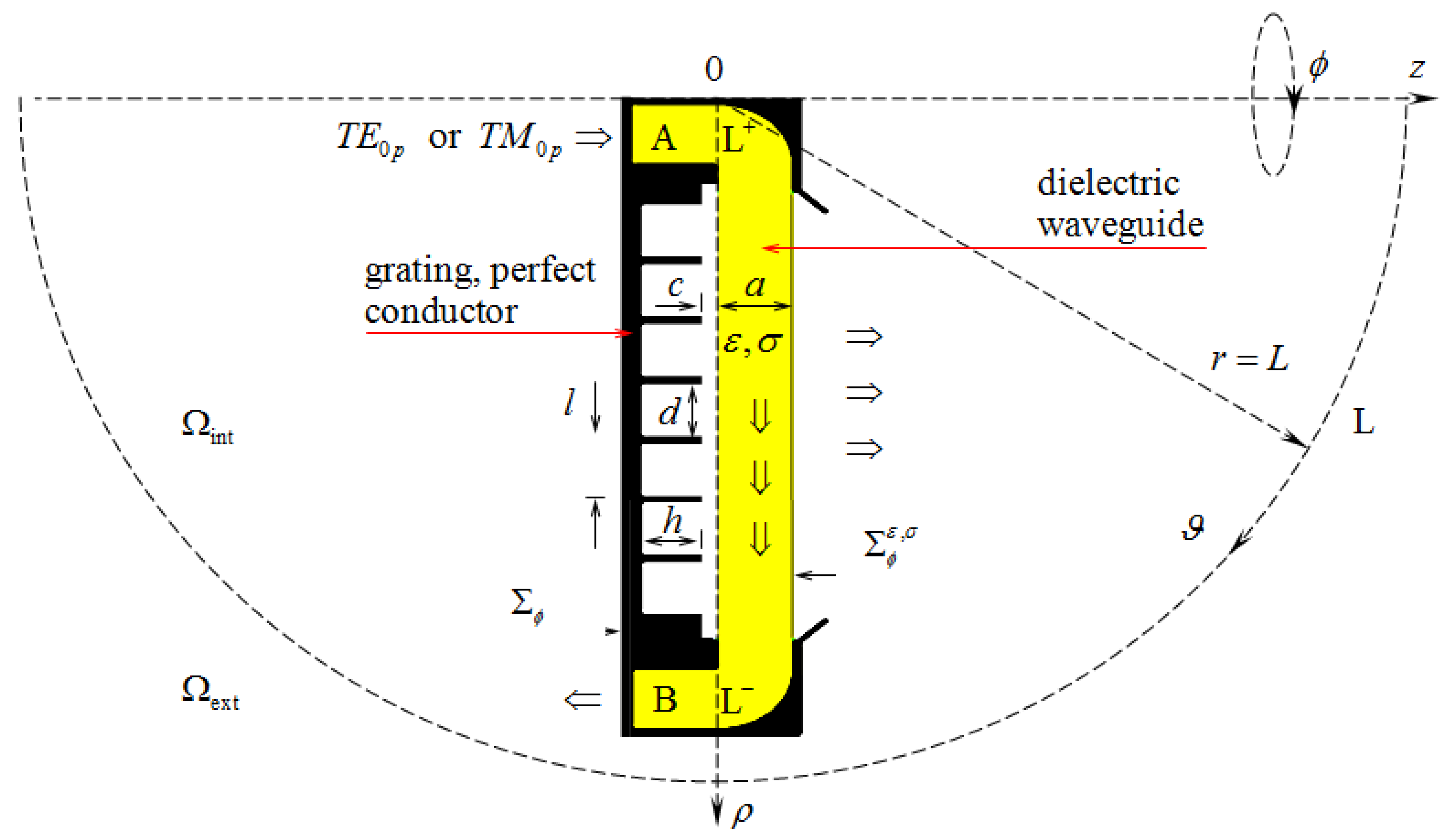
4. Radial Emitters with a Narrow Funnel-Shaped Radiation Pattern

It is possible that the implementation of wave analogs of Smith–Purcell coherent radiation in axially symmetric structures, which is going to be considered below, is the only fairly simple and least expensive way to build antennas with a very narrow funnel-shaped radiation pattern. The principle remains the same as with previously designed linear and planar antennas: the eigen slow wave of an open guiding line ‘sweeps out’ the periodic structure, and spatial propagating harmonics create the radiation field. The peculiarity lies in the fact that the role of an open guiding line is assigned to a planar radial dielectric waveguide, and a grating with concentric guiding lines, determining its period $l$, is put on a round disc installed on the axis $z$. The synthesis of an emitter with a very narrow funnel-shaped radiation pattern is reduced to the search for such a periodic structure that could provide the required amplitude and phase distribution of the radiation field at its zero spatial harmonic if the condition

$$\vartheta \left(k\right)=-{\alpha }_0\left(k\right)=\arcsin \left({\mathsf{\Phi }}_0/k\right)=\arcsin \left(\gamma \left(k\right)-\lambda /l\right)\approx 0$$

(21)

holds. Here, $\gamma \left(k\right)=\overline{\chi }\left(k\right)/k$ and $\overline{\chi }\left(k\right)={\mathsf{\Phi }}_1\left(k\right)$ are deceleration coefficient and propagation constant of the eigen surface wave of a radial dielectric waveguide, in which component $E_{\varphi }$ (in the case of $T{E}_0$-waves) or $H_{\varphi }$ (in the case of $T{M}_0$-waves) may be presented in the form $A\left(k,\rho ,z\right)\exp \left(i\overline{\chi }\left(k\right)\rho \right)$; ${\mathsf{\Phi }}_n\left(k\right)$ are longitudinal (along $\rho$) wavenumbers of grating’s spatial harmonics of the number $n$ [42,43,44]. Connecting values $\overline{\chi }\left(k\right)$ and ${\mathsf{\Phi }}_1\left(k\right)$, we implement in a form suitable for our particular case the well-known fact about the ‘identity’ of the field of the eigen surface wave of a planar dielectric waveguide and the field of one of the evanescent spatial harmonics of the grating [17,25,45]. This identity is manifested in the fact that the secondary fields of periodic structures generated by the fields of these generally different waves are the same. This allows us, when solving problems of analysis and synthesis of diffraction radiation antennas, to proceed from the fact that the characteristic bursts of their radiation pattern functions, both in magnitude and in the corresponding values of the angular coordinate, correlate fairly well with the amplitudes and space orientation of the spatial harmonics of the secondary fields of infinite gratings excited by the corresponding evanescent spatial harmonic. The effectiveness and validity of the approach to the construction of diffraction radiation antennas based on such concepts have already been proven by all the previous experience of researchers working in this direction.

Condition (21) formally reflects all that discussed above. If, for some values of $k=2\pi /\lambda$, $\gamma \left(k\right)$, and $l$, in the secondary field of an infinite grating excited by the first evanescent harmonic, only the fundamental harmonic (harmonic with a number $n=0$) is propagating, then, in the half-plane ${\mathsf{\Omega }}_{\mathrm{total}}$, it will go into free space at an angle $\vartheta \left(k\right)=-{\alpha }_0\left(k\right)=\arcsin \left({\mathsf{\Phi }}_0/k\right)$ [44]. The equality $\arcsin \left({\mathsf{\Phi }}_0/k\right)=\arcsin \left(\gamma \left(k\right)-\lambda /l\right)$ follows from the relations $\overline{\chi }\left(k\right)={\mathsf{\Phi }}_1\left(k\right)$ and ${\mathsf{\Phi }}_n={\mathsf{\Phi }}_0+2\pi n/l$ [44]. Condition (21) allows for each given frequency value to determine the period of the grating $l\approx \lambda /\gamma \left(k\right)$, capable of forming, together with a radial dielectric waveguide, supporting the propagation of a surface wave with a deceleration coefficient $\gamma \left(k\right)$, a radiation field with the main lobe of the directional pattern ‘pressed’ to the axis $z$. The structure of the grating period or the value of the parameter $c$ at the local intervals of the coordinate $\rho$ variation, which add up to the interval of length $L$, determining the real dimensions of the aperture of the synthesized device, can be changed and is selected in such a way as to fulfill the known requirements [46], which ensure the radiation pattern of the required quality and are related to the implementation of a certain amplitude distribution of the radiation field. Below, we restrict ourselves to considering prototypes of emitters with an aperture determined by a relatively small size of $10l<L<30l$ (the structure of the grating period and the parameter $c$ are constant) and focus on clarifying the question of whether it is possible, in principle, to form a very narrow funnel-shaped radiation pattern by structures with a radial arrangement of the main functional elements: a grating and a dielectric waveguide (Figure 2).

In the prototype shown in Figure 2 (the proportions in the image of the details of all analyzed structures are preserved), the circular feeder waveguide $\mathrm{A}$ ($a=0.15$ is its radius) moved into a radial waveguide and then into an open waveguide—a dielectric one ($\epsilon =2.1$). A reflective grating with parameters $l=0.14$, $d=0.07$, and $h=0.07$ (width and depth of slots) was placed at a distance $c=0.03$ from the dielectric waveguide. The period length $l$ is determined from condition (21) after calculating the propagation constants $\overline{\chi }\left(k\right)$ of a surface wave excited in a radial dielectric waveguide by a $T{E}_{01}$-wave of a circular waveguide $\mathrm{A}$. Specifically, the value $\overline{\chi }\left(k\right)\approx 46.4$ for the frequency $k=35$ ($\gamma \left(k\right)=\overline{\chi }\left(k\right)/k\approx 1.33$) was taken into account. The values of $\overline{\chi }\left(k\right)$ we obtain by calculating the phase incursion $\psi \left(k\right)=\arg \tilde{U}\left(g_2,k\right)-\arg \tilde{U}\left(g_1,k\right)=\overline{\chi }\left(k\right)$ of the field $\tilde{U}\left(g,k\right)$ caused by the displacement of the observation point along the dielectric waveguide axis $z=const$ from the point $g_1=\left\{z,{\rho }_1\right\}$ to the point $g_2=\left\{z,{\rho }_2\right\}$, ${\rho }_2-{\rho }_1=1.0$ [17,25]. According to the concepts discussed above, the considered emitter at frequencies close to $k=35$ should form a diagram, with one of the lobes directed practically along the axis $z$. This is true in a flat $\varphi =const$ representation. The rotation of this beam with variation of the coordinate $\varphi$ generates a ‘funnel’ in space, which we would like to see in the field’s distribution emitted by the antenna.

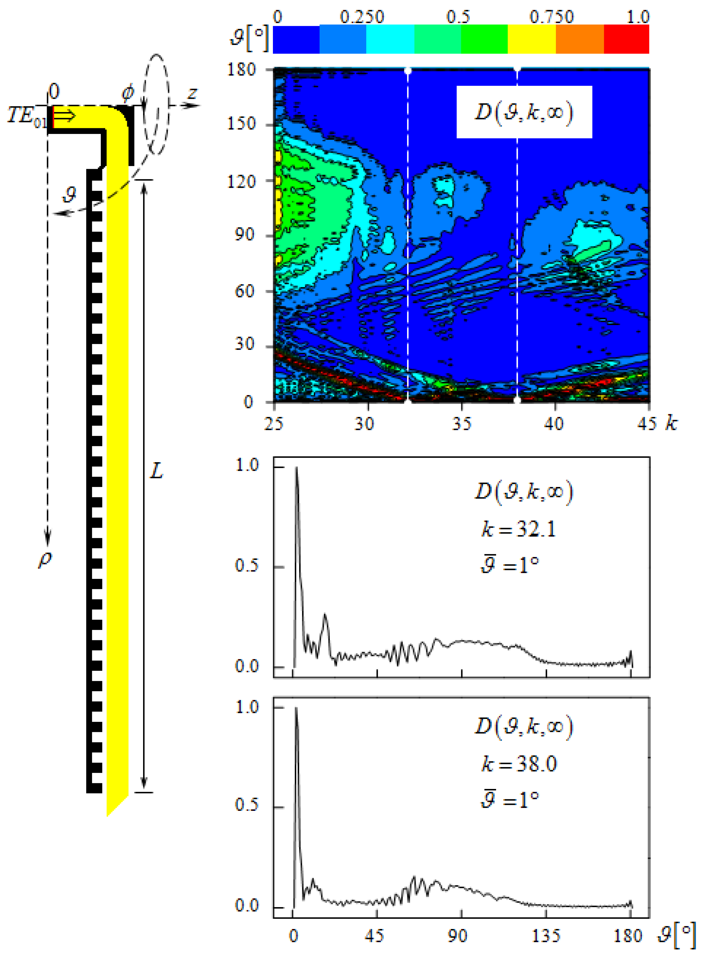
The results of numerical simulation in the frequency band $25\le k\le 45$ (in the waveguide $\mathrm{A}$, not more than two $T{E}_{0n}$-waves are propagating: $k_1^{+}\approx 17.7$, $k_2^{+}\approx 32.3$, $k_3^{+}\approx 46.8$; hereafter, the frequencies $k_n^{\pm }$ are the cut-off points of $T{E}_{0n}$- and $T{M}_{0n}$-waves in the waveguides $\mathrm{A}$ and $\mathrm{B}$, i.e., ${\gamma }_n^{\pm }\left(k_n^{\pm }\right)=0$) confirmed the expectations (Figure 2). The main and well-pronounced lobes of the radiation patterns at frequencies $k$ close to $k=32$ and $k=38$ are oriented in the direction $\vartheta =1°$. However, instead of one arc in the plane $\left\{k,\vartheta \right\}$ associated with the zeroth spatial harmonic of the grating propagating without attenuation, we see two shifted relative to each other in frequency and intersecting in the region $k\approx 35$. This allows us to conclude that not one but two competing surface waves with close values $\overline{\chi }\left(k\right)$ are excited in a dielectric waveguide, and in our calculations, we determined their average value.

The considered model did not allow to determine the radiation efficiency in the directions of interest, since a significant part of the energy, as seen from Figure 2, leaves the open end of the radial dielectric waveguide into the corner sector $50°<\vartheta <120°$. In other models presented in this section, we have corrected this drawback by adding a coaxial waveguide $\mathrm{B}$, removing the remained and not the radiated part of the primary $T{E}_{01}$-wave energy (Figure 3).

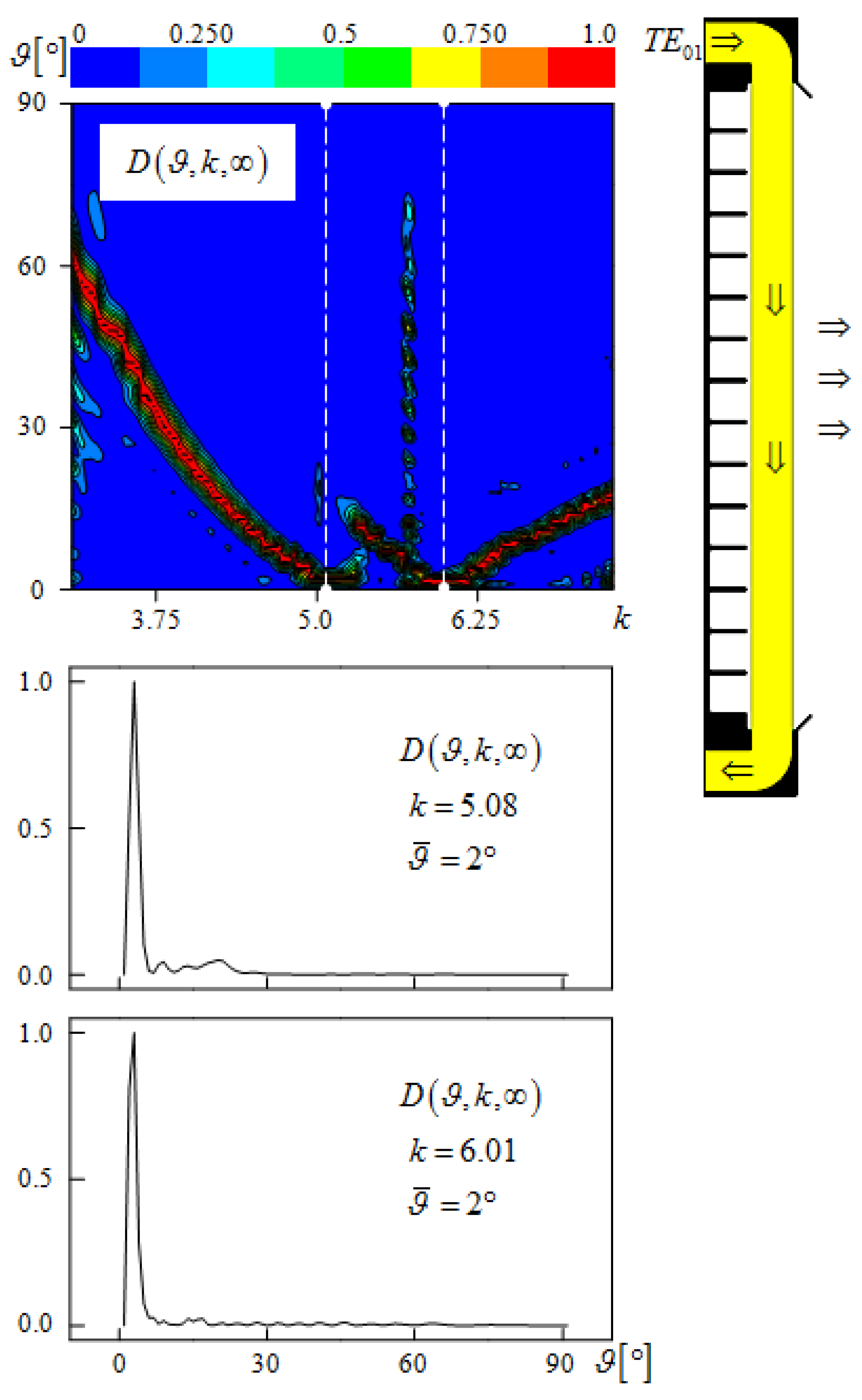
The propagation constants $\overline{\chi }\left(k\right)$ of the radial dielectric waveguide were calculated for the structure (see Figure 3) with following parameters: the radii $b^{\pm }$ of the inner conductors of the coaxial waveguides $\mathrm{A}$ and $\mathrm{B}$ are equal to 0.12 and 15.84, respectively; the radii $a^{\pm }$ of their outer conductors are 1.0 and 16.72; and the thickness of the radial dielectric ($\epsilon =2.1$) waveguide is equal to 0.88. The cutoff points of the first three $T{E}_{0n}$-waves in the waveguide $\mathrm{A}$ are equal to $k_1^{+}\approx 2.75$, $k_2^{+}\approx 5.14$, and $k_3^{+}\approx 7.55,$ and in the waveguide $\mathrm{B}$, $k_1^{-}\approx 2.46$, $k_2^{-}\approx 4.93$, and $k_3^{-}\approx 7.39$. For the analysis, a frequency band $3.1\le k\le 7.3$, where no more than two $T{E}_{0n}$-waves can propagate in each of these waveguides without attenuation, was chosen. At the frequency $k=5.2$, the average for this range, $\overline{\chi }\left(k\right)=6.96$, $\gamma \left(k\right)=\overline{\chi }\left(k\right)/k\approx 1.34$, and the value $l$ satisfying condition (21) is 0.9. Let us load an open dielectric waveguide with a reflective grating with defined above period $l=0.9$ and $d=h=0.8$ (aiming distance between the waveguide and the grating is $c=0.1$) and excite the structure with a pulsed $T{E}_{01}$-wave, such that

$$\begin{array}{l}{V}_1\left(g,t\right): v_1\left(z: g\in {\mathrm{L}}^{+},t\right)=4\frac{\sin \left[\mathsf{\Delta }k\left(t-\tilde{T}\right)\right]}{\left(t-\tilde{T}\right)}\cos \left[\tilde{k}\left(t-\tilde{T}\right)\right]\chi \left(\overline{T}-t\right)=F_1\left(t\right);\\ \tilde{k}=5.2, \mathsf{\Delta }k=2.1, \tilde{T}=50, \overline{T}=100.\end{array}$$

(22)

Here, $\chi \left(\dots \right)$ is the Heaviside step function, $\tilde{k}$ is the central frequency of the pulse $F_1\left(t\right)$, $\tilde{T}$ and $\overline{T}$ are its delay time and duration. The pulse $F_1\left(t\right)$ occupies the frequency band $\tilde{k}-\mathsf{\Delta }k\le k\le \tilde{k}+\mathsf{\Delta }k$ [31,34]; in our case, this is a chosen for analysis interval $3.1\le k\le 7.3$.

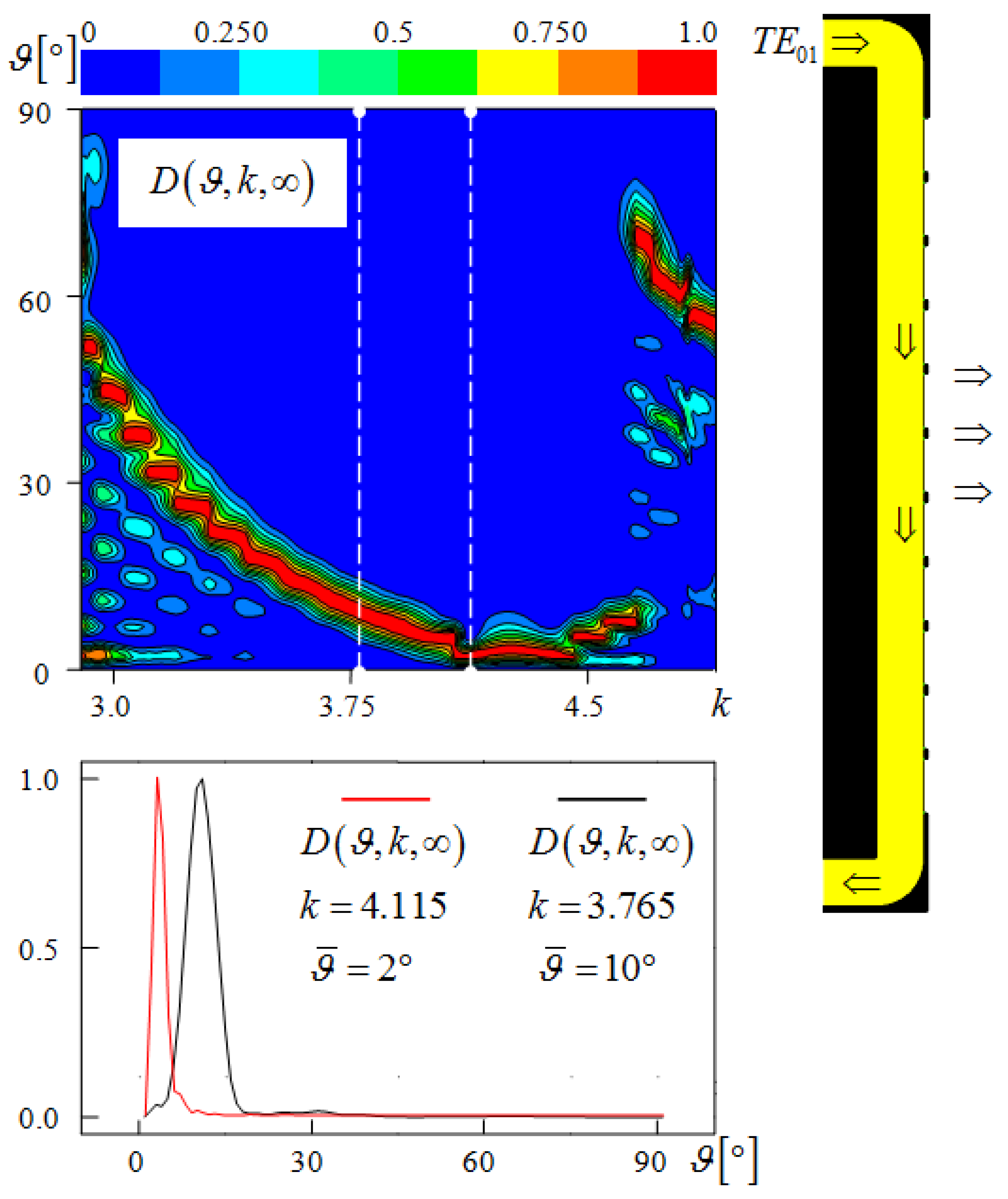
The numerical results are presented in Figure 4. Directional properties of the emitter are much better than in the case considered above—sufficiently ‘powerful’ side lobes in the radiation pattern are almost completely absent. The minimum deviation of the beam corresponding to the zero spatial harmonic of the grating from the axis $z$ was, in this case, equal to $2°$.

The lower fragments of Figure 4 show the dependences $D\left(\vartheta ,k,\infty \right)$ at frequencies $k=5.08$ and $k=6.01$; the radiation efficiency here is, respectively, $\eta \left(k\right)=0.43$ and $\eta \left(k\right)=0.17$. It is clear that, at least with the achieved value of $\eta \left(k\right)=0.43$ and the selected type of periodic structure, one can count on a successful solution of the problem associated with the formation of the required amplitude distribution of the radiation field of the antenna, having an aperture size several times larger than the aperture size $L$ of the considered prototype [17,20,25].

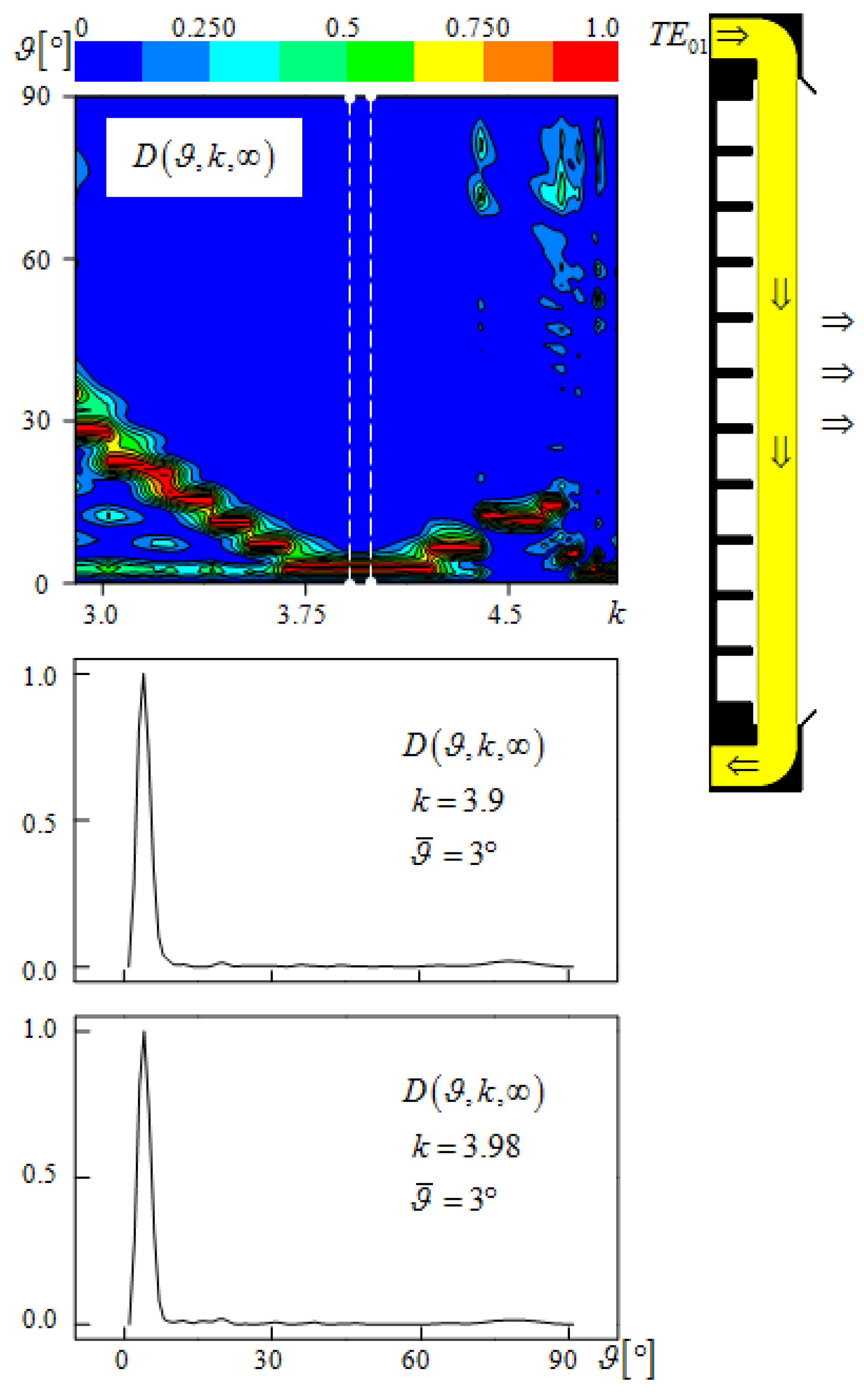
The upper fragment of Figure 4 tells us that a decrease in frequency (transition to the range $2.9\le k\le 4.9$, where only $T{E}_{01}$-waves propagate without attenuation in feeder coaxial waveguides $\mathrm{A}$ and $\mathrm{B}$) will allow us to get rid of the ‘two arcs’ effect in the radiation pattern of the emitter, discussed earlier. This should also change the size $l$ of the period of the grating, directing its fundamental spatial harmonic at an angle $\vartheta$ close to zero. So, for the value $k=3.9$, we obtain $\overline{\chi }\left(k\right)=5.14$ (see Figure 3), $\gamma \left(k\right)=\overline{\chi }\left(k\right)/k\approx 1.32$, and $l=2\pi /k\gamma \left(k\right)\approx 1.22$.

Having loaded the radial waveguide with a grating of a period $l=1.2$ ($d=1.0$, the parameters $h$ and $c$ remain the same) and having excited the structure with a pulsed $T{E}_{01}$-wave $V_1\left(g,t\right): v_1\left(z: g\in {\mathrm{L}}^{+},t\right)=F_1\left(t\right),$ $\tilde{k}=3.9$, $\mathsf{\Delta }k=1.0$, $\tilde{T}=50$, and $\overline{T}=100$, we arrive at the results presented in Figure 5. These results fully meet our expectations, but the minimum deviation of the beam corresponding to the zero spatial harmonic of the grating from the axis $z$ has increased to $3°$. Obviously, this is due to a decrease in the number of grating periods that fit into the length $L$, determining the dimensions of the emitter aperture. With the transition to a full-size aperture of the synthesized antenna, this indicator can be significantly improved.

As it has already been noted more than once [17,20,25], for the successful solution of the problem of synthesizing a real antenna of diffraction radiation, the energy parameters $\eta \left(k\right)$ of prototype emitters and the ability to control their change by varying one of the parameters $d$, $h$, or $c$, are important. In the case under consideration, $\eta \left(k\right)=0.41$ at frequency $k=3.9$, and $\eta \left(k\right)=0.43$ at $k=3.98$. Figure 6 shows how the radiation intensity changes with a change in the aiming distance $c$, that is, the distance between the grating and the radial dielectric waveguide. When performing a specific technical task for the construction of a diffraction radiation antenna, similar dependences, calculated for all admissible (not leading to phase distortions of the surface wave field [17,20,25]) values $c$ should be taken into account.

An important issue in the construction of real antennas is the question of maximum simplification of their design without losses in the quality of the main electrodynamic characteristics of devices. In part, this also holds for the used periodic structures. The parameters of far from all gratings of classic geometry (gratings of the ‘comb’ type, for example) can be strictly maintained during their manufacture and operation in the wavelength ranges from 3.0 mm and less. A prototype of a diffractive radiation antenna, the main electrodynamic characteristics of which are presented in Figure 7 and Figure 8, can be proposed as one of the options allowing to effectively solve the above problems.

In this prototype, one of the planes of the radial dielectric waveguide is metallized, and the second one contains a concentric grating of ‘thick’ ($h=0.08$) narrow ($l-d=0.2$, $l=1.2$) metal strips—its propagating spatial harmonics mainly form the radiation field. The structure is excited by a pulsed $T{E}_{01}$-wave $V_1\left(g,t\right): v_1\left(z: g\in {\mathrm{L}}^{+},t\right)=F_1\left(t\right)$, $\tilde{k}=3.9$, $\mathsf{\Delta }k=1.0$, $\tilde{T}=50$, $\overline{T}=100$, covering the frequency range $2.9\le k\le 4.9$. For the expected value $k=3.9$, the minimum deviation of the main lobe of the radiation pattern from the axis $z$, equal to $2°$, is obtained for frequencies $4.09\le k\le 4.15$. The radiation pattern characteristic of this range is shown in the upper fragment of Figure 7. For $k=4.115$, radiation efficiency is $\eta \left(k\right)=0.34$. The frequency $k=3.765$ corresponds to the maximum efficiency $\eta \left(k\right)=0.97$; the corresponding radiation pattern is shown in the bottom fragment of Figure 7.

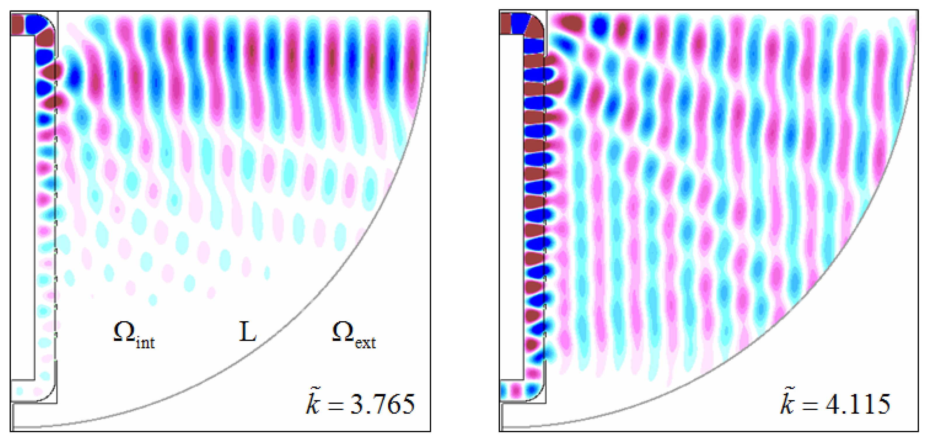
Figure 8 shows the spatial distribution of the radiation field at the instant $t=125$, when the structure is excited by a quasi-monochromatic $T{E}_{01}$- pulse wave:

$$\begin{array}{l}{V}_1\left(g,t\right): v_1\left(z: g\in {\mathrm{L}}^{+},t\right)=P\left(t\right)\cos \left[\tilde{k}\left(t-\tilde{T}\right)\right]=F_2\left(t\right);\\ P\left(t\right)= 0.01-5-95-99, \tilde{T}=0.5, \tilde{k}=3.765 \mathrm{and} \tilde{k}=4.115\end{array}$$

(23)

where $\tilde{k}$ is the central frequency of the signal $F_2\left(t\right)$ and $P\left(t\right): t_1-t_2-t_3-t_4$ is its trapezoidal envelope, which equals unit for $t_2<t<t_3$, and is zero for $t<t_1$ and $t>t_4.$ The fronts of the radiated waves are practically flat (in the representation for values $\varphi =const$) and the orientation of the relevant planes corresponds to the previously determined values $\overline{\vartheta }=10°$ (for $k=3.765$) and $\overline{\vartheta }=2°$ (for $k=4.115$). Obviously, the non-uniform (especially in the case $\tilde{k}=3.765$) distribution of the radiation field amplitude along the emitter aperture is connected, among other things, with a decrease in the spatial energy density carried by the surface wave of the radial waveguide as it moves along the axis $\rho$. It will be necessary to consider the corresponding effect when creating actual antennas with a sufficiently large value of $L$ determining the size of their apertures.

5. Conclusions

The paper briefly describes rigorous models of the method of exact absorbing conditions, enabling the study and analysis of the effects of diffraction radiation (wave analogs of the effects of SPR) in axially symmetric electrodynamic structures such as ‘a finite segment of an open radial guiding line installed near a finite concentric reflective or semitransparent grating’. These mathematical models, implemented in a complex of original authentic algorithms and codes, were used to study the physics of the processes of transformation of eigen surface waves of the corresponding open waveguides into waves propagating infinitely far in free space. The primary attention was paid to emitters—prototypes of practical antennas, capable of forming a funnel-shaped radiation pattern with a very narrow ‘throat’. The results discussed in the paper confirm the possibility to construct such well-directed antennas, implementing the wave analog of the Smith–Purcell coherent radiation. The presented results also prove the correctness of our ideas about how, in what way, and due to what physical principals the proposed for implementing non-standard transformations of electromagnetic waves structure should work. It has been shown how and within what limits the characteristics of the corresponding devices can be changed in a controlled manner. In particular, this may be performed by the optimal selection of the parameters of the open waveguide line (due to the change in the parameters of the surface waves directed by such a line) and/or by choosing the geometric and material parameters of the grating, as only gratings propagating spatial harmonics determine all the features of the radiation field.