An Improved Image Filtering Algorithm for Mixed Noise

Abstract

In recent years, image filtering has been a hot research direction in the field of image processing. Experts and scholars have proposed many methods for noise removal in images, and these methods have achieved quite good denoising results. However, most methods are performed on single noise, such as Gaussian noise, salt and pepper noise, multiplicative noise, and so on. For mixed noise removal, such as salt and pepper noise + Gaussian noise, although some methods are currently available, the denoising effect is not ideal, and there are still many places worthy of improvement and promotion. To solve this problem, this paper proposes a filtering algorithm for mixed noise with salt and pepper + Gaussian noise that combines an improved median filtering algorithm, an improved wavelet threshold denoising algorithm and an improved Non-local Means (NLM) algorithm. The algorithm makes full use of the advantages of the median filter in removing salt and pepper noise and demonstrates the good performance of the wavelet threshold denoising algorithm and NLM algorithm in filtering Gaussian noise. At first, we made improvements to the three algorithms individually, and then combined them according to a certain process to obtain a new method for removing mixed noise. Specifically, we adjusted the size of window of the median filtering algorithm and improved the method of detecting noise points. We improved the threshold function of the wavelet threshold algorithm, analyzed its relevant mathematical characteristics, and finally gave an adaptive threshold. For the NLM algorithm, we improved its Euclidean distance function and the corresponding distance weight function. In order to test the denoising effect of this method, salt and pepper + Gaussian noise with different noise levels were added to the test images, and several state-of-the-art denoising algorithms were selected to compare with our algorithm, including K-Singular Value Decomposition (KSVD), Non-locally Centralized Sparse Representation (NCSR), Structured Overcomplete Sparsifying Transform Model with Block Cosparsity (OCTOBOS), Trilateral Weighted Sparse Coding (TWSC), Block Matching and 3D Filtering (BM3D), and Weighted Nuclear Norm Minimization (WNNM). Experimental results show that our proposed algorithm is about 2–7 dB higher than the above algorithms in Peak Signal-Noise Ratio (PSNR), and also has better performance in Root Mean Square Error (RMSE), Structural Similarity (SSIM), and Feature Similarity (FSIM). In general, our algorithm has better denoising performance, better restoration of image details and edge information, and stronger robustness than the above-mentioned algorithms.

1. Introduction

Images are inevitably affected by noise during the process of acquisition, storage, recording, and transmission, which reduces the image contrast and seriously affects the application of images [1]. For most images, the noise mainly comes from Gaussian noise and impulse noise. In many cases, the two types of noise appear at the same time. Gaussian noise comes from electronic circuit noise and sensor noise caused by low lighting or high temperature. It has the characteristics of high density and a wide fluctuation range of noise intensity [2]. Impulse noise is also called salt and pepper noise, which is generated by the image sensor, transmission channel, decoder, etc., and appears as black and white spots on the image. In the process of image denoising, the main factor to be considered is to ensure the integrity of image features while removing noise. These features mainly include the information of image edge, image contour, image texture, and image color, etc.

Traditional filtering algorithms are mainly divided into two categories: spatial domain and frequency domain [3]. The spatial domain method processes the image pixels directly, and traditional spatial filtering includes median filtering, mean filtering, Gaussian filtering, and bilateral filtering. The frequency domain method transforms the original image into the frequency domain through integral transformation, then deals with the image in the frequency domain and finally transforms it into the spatial domain inversely to enhance the image and achieve the purpose of denoising. Traditional frequency domain filtering includes Fourier transform, discrete cosine transform, wavelet transform, and multi-scale geometric analysis, etc.

Among all the algorithms for removing salt and pepper noise in images, traditional median filtering is a commonly used and effective method. The algorithm uses the median value of pixels in the neighborhood of a small window to replace the gray value of each pixel in the original image, which has a good effect on suppressing impulse noise. The image edge and other details can be better maintained. The disadvantage is that the algorithm uses the neighborhood median to replace all pixels of the noise image, which makes the algorithm’s filtering performance drop sharply under the condition of high-density noise pollution, and even loses its denoising performance, and the edges are prone to shift and the texture details are not clear. For this reason, some improved median filtering algorithms [4,5,6,7,8] have been proposed. These algorithms improve the performance of median filtering to a certain extent and can filter out salt and pepper noise with high density; however, the protection of image edge details is still not ideal. Reference [9] is an improved Adaptive Median Filter (AMF) algorithm, which can adjust the size of the filter window according to the noise density, but it is easy to misjudge the extreme point as a noise point to filtering. Reference [10] is another improved adaptive median filtering algorithm. Based on the idea of maximum–minimum median filtering, the algorithm uses a two-level detection method to accurately divide pixels into signal points and noise points, so as to filtering image noise effectively. Reference [11] proposed an improved multilevel median filtering algorithm (VHWR). The algorithm can better maintain the image details, greatly improve the filtering effect of salt and pepper noise with high density. However, the denoising effect is not satisfactory when the noise density is too high.

Since Donoho et al. proposed the hard threshold function [12] and the soft threshold function [13], the wavelet threshold denoising algorithm has been widely used. However, the discontinuity of the hard threshold function will cause the reconstructed image signal to oscillate, and the fixed deviation of the soft threshold function will result in blurry or excessively smooth borders to the denoised image. A large number of scholars have proposed many improved wavelet threshold functions to achieve a more accurate denoising effect [14,15,16,17,18,19]. Reference [20] proposed a new wavelet threshold algorithm that overcomes the problems of fixed deviation and discontinuity in the traditional wavelet threshold function, and improves the wavelet threshold function and the threshold. Reference [21] combines the advantages of the joint regularization restoration method of spatial local threshold processing and wavelet domain processing and can achieve good results in effectively suppressing noise and artifacts. Reference [22] takes advantage of the merits of traditional Wiener filtering in the wavelet domain to deal with mixed noise, and it carries out improved Wiener filtering based on multi-directional weighting, so that the algorithm can well maintain the detailed features of the original image and further improve the peak signal-to-noise ratio of the output image. Reference [23] has studied the multi-resolution method of Haar wavelet transform for medical image denoising. It applies Haar transform to each two-dimensional image layer separately and evaluates the whole image using three-dimensional technology. This method benefits from the similarity between adjacent image layers and has a reasonable denoising effect. Reference [24] proposed a wavelet denoising method based on an unsupervised learning model. The method uses the advantages of wavelet transform and uses an unsupervised dictionary learning algorithm to create a dictionary for noise reduction, which shows very competitive denoising performance. Reference [25] presented improvements in image gap restoration through the incorporation of edge-based directional interpolation within multi-scale pyramid transforms and reconstructed two types of image edges. Reference [26] shows how to design a complex wavelet with good characteristics based on the important characteristics of dual-tree complex wavelet transform and explains a series of applications of dual-tree complex wavelet in signal and image processing.

Buades et al. [27] proposed the Non-local Means (NLM) denoising algorithm in 2005. By utilizing the repeatability and self-correlation within an image, the algorithm first calculates the weighted average value of the neighborhood of all pixels in the image and the neighborhood of the current pixel, then takes the average value as the Euclidean distance between the two points and assigns weights to them through the weight function. The sum of the product of the weight and all pixels is the denoised value of the current pixel. However, the NLM algorithm still has an unsatisfactory denoising effect on excessively high noise; therefore, many new algorithms have been proposed [28,29,30,31,32,33]. Reference [34] separates noise components from image information using Principal Component Analysis (PCA), improves the accuracy of similarity measurement of NLM algorithm, and achieves a good denoising effect. Reference [35] proposes a new NLM algorithm based on similarity confirmation. The algorithm first determines the threshold according to the distance distribution between image blocks, and it then uses the reserved image blocks to realize denoising. Reference [36] designed a new similarity weight function using the residual image information in the method noise and achieved good denoising effect. Reference [37] uses an improved NLM algorithm to solve the problems of long time-consuming, unreasonable weight distribution and failure to highlight the role of central pixels when calculating the similarity between neighborhoods by Euclidean distance. The algorithm can measure the neighborhood similarity more accurately and better retain the edge and detail information of the image when removing Gaussian noise. The denoising effect of noised images is further improved. In recent years, denoising algorithms based on sparse regularization have attracted the attention of many scholars due to their characteristics of over-completeness and sparsity. Elad et al. [38] proposed a denoising algorithm of sparse representation KSVD, which makes full use of the advantages of sparse representation and can well preserve the edge of the image while denoising. The algorithm assumes that the structural elements of the image can be expressed by a set of super-complete dictionary atoms. The dictionary atoms are used to reconstruct the image to remove redundancy and achieve the purpose of denoising. However, the algorithm is only suitable for removing slightly polluted noise images. In the case of serious noise pollution, the image denoising effect is not very satisfactory. In order to further improve the denoising effect, reference [39] proposed a Non-locally Centralized Sparse Representation (NCSR) algorithm. The algorithm introduces the concept of sparse coding noise to transform the solution target of the model from acquiring the original image to suppressing the sparse coding noise of the image, and it makes full use of the nonlocal self-similarity of the image to obtain a good estimate of the sparse coding coefficient of the original image. The algorithm can still achieve a good denoising effect when the noise pollution is serious. Reference [40] proposed a denoising algorithm, OCTOBOS, which can adaptively learn the structured incomplete sparse transform with block sparsity (or the equivalent union of square sparse transform), and cluster the data through sparse coding at the same time. Reference [41] proposed a Trilateral Weighted Sparse Coding (TWSC) scheme for real image denoising. TWSC introduces three weight matrices into the data and regularization terms of the sparse coding framework to describe the statistical characteristics of the real noise and image prior model, and it uses the alternating direction method of multiplier to solve the problem. TWSC also has a reasonable denoising performance. Although the denoising effect is good, the iteration and updating of dictionary learning lead to a large amount of calculation and high time cost. Considering the above problems, Dabov et al. [42] proposed a more efficient and higher sparsity transform domain sparse expression method, namely Block Matching and 3D Filtering (BM3D). BM3D utilizes the correlation between “blocks” to achieve a high degree of sparseness of images through joint filtering, with better denoising performance, higher operating efficiency, and more advantages than other methods.

Due to the development of convex and non-convex optimization methods, matrix low-rank approximation has also attracted the attention of many scholars, and many important models and algorithms have been proposed. Rank minimization is one of the important research directions. Because rank minimization is an NP-hard problem [43], it is easy to solve using the nuclear norm of the matrix as the convex relaxation optimization target of the matrix rank, and this method is called Nuclear Norm Minimization (NNM). NNM has developed rapidly, both in theory and in application. Gu et al. [44] proposed the Weighted Nuclear Norm Minimization (WNNM) algorithm to optimize NNM, which assigns different weights to singular values with different values, that is, the larger the singular value, the larger the weight, and the larger the proportion. The algorithm is more effective in removing the noise of natural images.

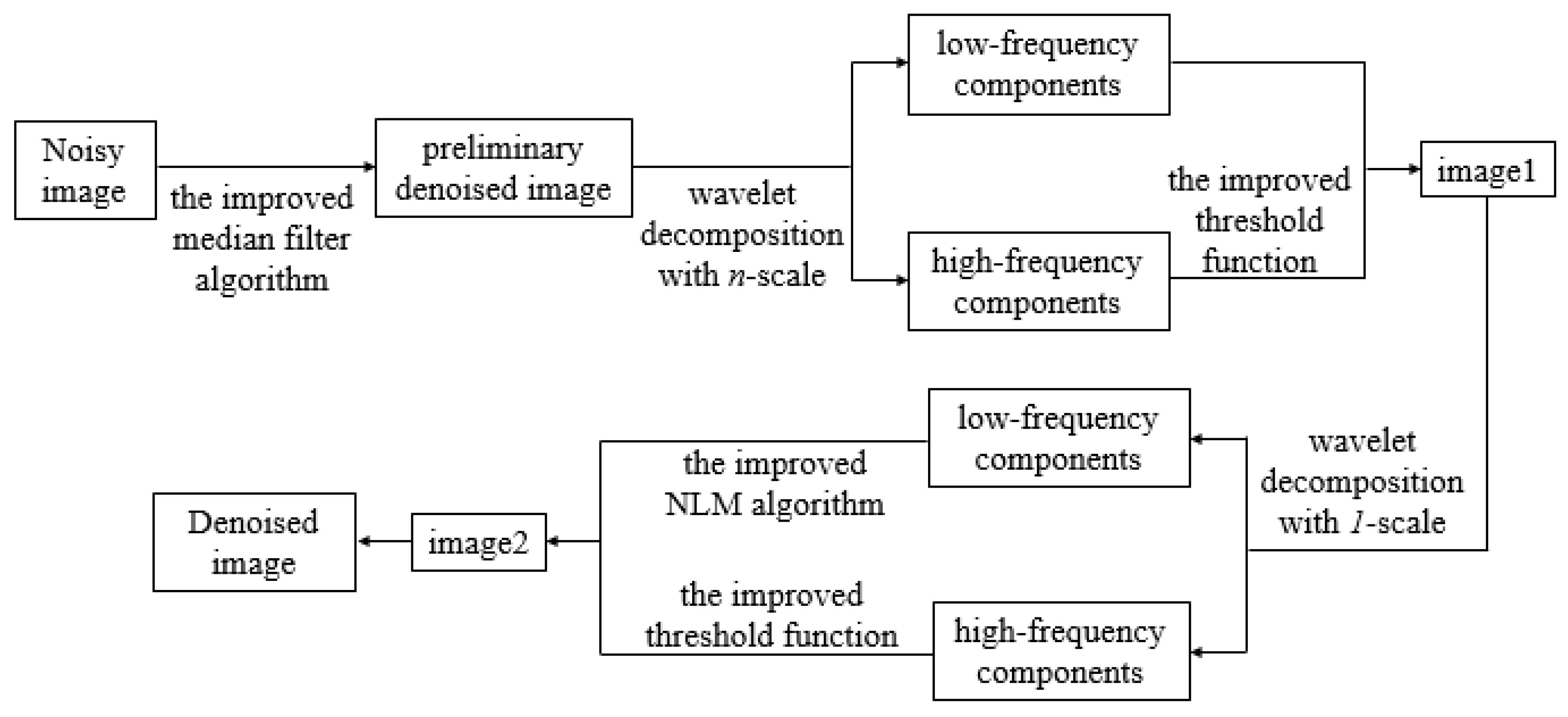
In view of the mentioned problems above and the status quo of denoising algorithms, this paper proposes a new denoising algorithm for salt and pepper + Gaussian noise based on reference [10], reference [20], and reference [37]. The algorithm first uses the improved median filter algorithm to denoise the original image with mixed noise, which can filter out most of the salt and pepper noise, and then performs n-scale wavelet decomposition on the filtered image. The high-frequency components of each subsequent layer are processed by the improved wavelet threshold algorithm to achieve preliminary removal of Gaussian noise. The processed high-frequency components and unprocessed low-frequency components are then reconstructed. After that, the wavelet decomposition on the reconstructed image is performed with 1-scale, and the improved NLM algorithm is used to process the low-frequency components, which can filter out the noise information remaining in the low frequency components. At the same time, the high-frequency components continue to be processed with the improved wavelet threshold algorithm to further filter out the noise remaining in the high-frequency components. Finally, the low-frequency components and the high-frequency components are again reconstructed to obtain the final denoised image. Experimental results show that the proposed algorithm has a better denoising effect and finer detail restoration ability, both from subjective evaluation and objective evaluation metrics, compared with the algorithms mentioned above.

2. The Filtering Algorithm for Mixed Noise with Salt and Pepper + Gaussian Noise

In this section, we will introduce and analyze the proposed filtering algorithm with mixed noise in detail. This algorithm involves the improvement of three sub-algorithms:

• We made improvement to the traditional median filtering algorithm. Compared with the Adaptive Median Filtering (AMF) algorithm, the weighted multilevel median filtering algorithm, and the multilevel nonlinear weighted mean median filtering algorithm, the improved algorithm has better filtering effect for salt and pepper noise.
• We improved the wavelet threshold denoising algorithm’s threshold function and threshold. This improved algorithm has better removal effect on Gaussian noise than the traditional hard threshold denoising, soft threshold denoising, and semi-soft threshold denoising algorithms.
• We made improvements in the Euclidean distance function that measures the similarity of image blocks in the NLM algorithm, and the distance weight function between similar image blocks. The improved algorithm performs better in filtering Gaussian noise than the NLM algorithm and can better preserve the edge and detail information of the image.

The three improved sub-algorithms are combined to denoise salt and pepper + Gaussian noise according to a certain process. Experimental results show that the algorithm is robust and has excellent denoising ability and detail recovery ability.

2.1. The Improved Median Filtering Algorithm

Median filtering is a classical nonlinear filtering method. It sets the gray value of a pixel point to the median gray value of all pixels in the neighborhood window centered on the point, which is very effective for eliminating salt and pepper noise. Traditional median filtering uses a fixed-size filtering window to sorts all the pixels in the window to find the median value, and it then replaces the center pixel value of the window with the median value. Even if the window center value is not noise, it is still replaced, resulting in the details and edge of image to be blurred.

The algorithm proposed in this paper improves the traditional median filtering algorithm. All pixels of the image are accurately divided into signal points and noise points by the method of two-level detection, and only noise points are processed. The algorithm uses 3 × 3 filtering windows. If the median value of the pixels in the window is not the noise value, the center noise is replaced by the median value; otherwise, the center noise is not processed. This is carried out repeatedly with the corresponding 3 × 3 window in the whole image until there is no noise in the image or the noise cannot be filtered out with a 3 × 3 window. If there are still large noise blocks in the image, the noise points in the noise blocks are replaced by the mean value of the adjacent signal points.

The boundary pixels of the noisy image are copied and filled out for the purpose of denoising, so that the size of the noisy image is expanded from M ∗ N to (M + 2) ∗ (N + 2). When the denoising process is finished, the extra pixels can be deleted to obtain the correct image size.

2.1.1. First-Level Detection of Noise Point

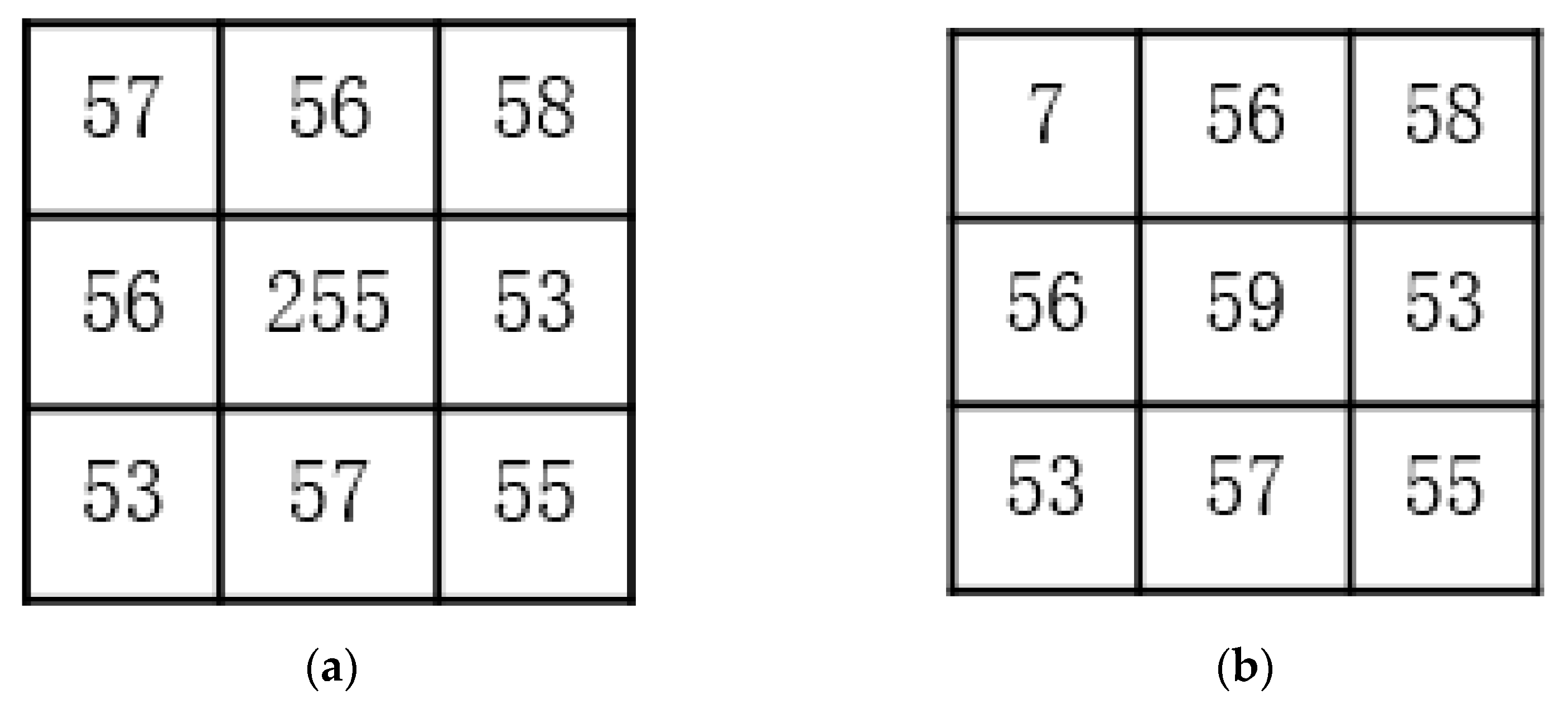
Salt and pepper noise points generally represent the maximum or minimum value of the local area of the image, the positions of the contaminated pixels are randomly distributed, and the probability of positive and negative noise points is usually equal. Image noise points are often extreme points in local areas, but extreme points in local areas are not necessarily noise points. As shown in Figure 1a, the central pixel is the maximum value of the 3 × 3 neighborhood. It differs greatly from the surrounding pixel value and can be considered as a noise point, while the central pixel value in Figure 1b is still the maximum value. It has little difference from the surrounding pixel values and should be considered as a signal point.

Set $f_{i,j}$ is the gray value of the center pixel of the 3 × 3 window and $w^3$, $w_{max}^3$ and $w_{min}^3$ represent, respectively, the maximum gray value and the minimum gray value of all pixels in window $w^3$. If $f_{i,j}=w_{max}^3$ or $f_{i,j}=w_{min}^3$, $f_{i,j}$ is marked as the possible noise point; otherwise, $f_{i,j}$ is marked as the signal point. The following formula is constructed:

$$flag\left(i,j\right)=\{\begin{array}{c}1, f_{i,j}=w_{max}^3 \mathrm{or} f_{i,j}=w_{min}^3\\ 0, f_{i,j}\ne w_{max}^3 \mathrm{and} f_{i,j}\ne w_{min}^3\end{array}$$

(1)

2.1.2. Second-Level Detection of Noise Point

As mentioned above, local extreme points are not necessarily noise points. If all local extreme points are taken as noise points for median value replacement, the details will inevitably be lost. For a natural smooth image, the pixel values of the smooth area are similar or even equal. Only at the edge of the image, or in the area with rich details, are the difference of image pixel values relatively large. According to human visual characteristics, it is more sensitive to the noise in the smooth area than the noise in the detailed area. If the possible noise point is still an extreme point in a larger window, this point is considered as a noise point. Using a larger window to judge noise points can effectively improve the accuracy of noise detection.

In this paper, a 7 × 7 window is used for secondary confirmation of possible noise points. The 7 × 7 window is marked as $w^7$; $w_{max}^7$ and $w_{min}^7$ represent the maximum value and the minimum value of window $w^7$, respectively, and $f_{i,j}$ represents the possible noise of window $w^3$. If $f_{i,j}=w_{max}^7$ or $f_{i,j}=w_{min}^7$, then $f_{i,j}$ is marked as the noise point; otherwise, $f_{i,j}$ is marked as the signal point.

The following formula is constructed:

$$flag\left(i,j\right)=\{\begin{array}{c}1,(f_{i,j}=w_{max}^3 \mathrm{and} f_{i,j}=w_{max}^7) \mathrm{or} (f_{i,j}=w_{min}^3 \mathrm{and} f_{i,j}=w_{min}^7)\\ 0, \mathrm{otherwise}\end{array}$$

(2)

2.1.3. The Selection for Window Size

The selection of filtering window size will affect the filtering effect. A large window has a strong filtering ability but a weak detail preservation ability; a small window can retain many details of the image, but its filtering performance is bad. Selecting the filter window adaptively according to the size of the noise density can alleviate the contradiction between filter performance and detail preservation, but it also increases the time complexity of the algorithm.

If the median value in the 3 × 3 neighborhood window of a noise point is still noise, the filtering fails. If the neighborhood window is enlarged to 5 × 5 and the median value in the window is no longer noise, the filtering is successful after replacing the noise point with the median value. In fact, if a noise point cannot be successfully filtered using a 3 × 3 window, it can be put aside and used to process those noise points that can be successfully filtered using a 3 × 3 window. Once all noise points that can be filtered by a 3 × 3 window have been replaced with their corresponding median values, those noise points can no longer be processed before being filtered. Therefore, the filtering results of these two methods are the same. In our proposed algorithm, the size of the filtering window is selected as 3 × 3.

2.1.4. Processing of Noise Blocks

If the image is slightly polluted by noise, filtering with a 3 × 3 filtering window repeatedly can deal with all the noise. However, if the image is seriously polluted by noise, the larger noise blocks cannot be filtered by a 3 × 3 filtering window. As shown in Figure 2, 0 represents signal point and 1 represents noise point. The experimental results show that, when the noise density is less than 0.5, all noise can be removed by repeated filtering with a 3 × 3 filtering window.

For the noise in the noise block, the algorithm deals with it with mean filtering. For the noise outside the noise block, the algorithm replaces it with the mean gray value of its adjacent pixels. Figure 3 shows the four cases in which noise points are replaced by the mean gray values of adjacent pixels. Similarly, 1 represents noise point and 0 represents signal point.

Formula (3) shows the calculation method of noise point in the first case in Figure 3.

$$f_{i,j}=\frac{1}{3}\left(f_{i-1,j-1}+f_{i-1,j}+f_{i,j-1}\right)$$

(3)

2.1.5. The Implementation Process of the Algorithm

• Mark all the noise points in the image. If the (i,j) pixel is a noise point, then set $flag\left(i,j\right)=1$ and replace = 0.
• If $flag\left(i,j\right)=1$, obtain the median value Med of all pixels in the 3 × 3 window centered on point (i,j); If the median value Med is not noise, replace the central pixel of the 3 × 3 window with Med, set $flag\left(i,j\right)=0$ and replace $=1$; otherwise, the center pixel will not be processed.
• Finish processing all points with $flag\left(i,j\right)=1$ and output the results as the image to be processed.
• If replace $=1$, repeat steps (2) and (3); otherwise, it means that there is no noise in the image or there are large noise blocks but they cannot be processed by a 3 × 3 window.
• If ${\displaystyle \sum }flag\ne 0$, it indicates that there are still noise blocks in the image, and then the noise $f_{i,j}$ is replaced by the mean value of the adjacent signal points.
• Output the filtering results.

2.2. The Improved Wavelet Threshold Denoising Algorithm

Since Donoho et al. proposed the hard threshold function [12] and the soft threshold function [13], the wavelet threshold denoising algorithm has been widely used. However, the discontinuity of the hard threshold function will cause the reconstructed image signal to oscillate, and the fixed deviation of the soft threshold function will result in blurry or excessively smooth borders of the denoised image. Based on the soft and hard threshold functions, this algorithm proposes an improved threshold function that overcomes the discontinuity of hard threshold and the fixed deviation of soft threshold, reduces the compression of wavelet coefficients, and solves the problems of image oscillation and boundary blur to a certain extent. At the same time, the new threshold can change with the noise level of the high-frequency components in each layer of wavelet decomposition, which has strong flexibility and adaptability.

2.2.1. The Theory of Wavelet Threshold Denoising

Wavelet transform is a linear operation. After wavelet transform, the wavelet coefficients of noise image are equal to the sum of wavelet coefficients of the original image and the wavelet coefficients of noise. Separating noise means removing the wavelet coefficients of noise and retaining the wavelet coefficients of the original image in the wavelet domain.

After multi-scale wavelet decomposition, the wavelet coefficients of effective information of the image and the wavelet coefficients of noise have different characteristics. The part of low-frequency is wavelet approximation; the part of high-frequency is wavelet details. The effective information of image is mainly distributed in wavelet approximation; the high-frequency part mainly contains image edge and noise. The effective information of image is mainly concentrated in larger wavelet coefficients, while noise is mainly concentrated in smaller wavelet coefficients. With the increase of wavelet decomposition scale, the wavelet coefficients of the effective signal of the image become increasing larger, while the wavelet coefficients of noise information become increasing smaller. Therefore, the wavelet coefficients of the image between effective information and noise information tend to separate after repeated decomposition. According to this principle, image signal and noise signal can be separated.

Therefore, the process of wavelet threshold denoising can be summarized as follows: first decompose the original image with appropriate wavelet basis, and then select a proper threshold value to deal with noise, and finally reconstruct the wavelet coefficients to obtain an ideal denoised image.

It is very important to construct an appropriate threshold function and select a proper threshold. The threshold function commonly used is the one proposed by Donoho; the hard threshold function [12] and the soft threshold function [13] are shown in Formulas (4) and (5), respectively.

$${\tilde{W}}_{j,k}=\{\begin{array}{c}{W}_{j,k , } \left|W_{j,k}\right|\ge \lambda \\ 0, \left|W_{j,k}\right|<\lambda \end{array}$$

(4)

$${\tilde{W}}_{j,k}=\{\begin{array}{c}sign(W_{j.k})\left(\left|W_{j,k}\right|-\lambda \right), { }_{ }\left|W_{j,k}\right|\ge \lambda \\ 0, \left|W_{j,k}\right|<\lambda \end{array}$$

(5)

where $W_{j,k}$ is the k-th wavelet coefficient under the j-th scale of noise image after wavelet decomposition; ${\tilde{W}}_{j,k}$ is the wavelet coefficients obtained through threshold processing; $\lambda$ is the threshold selected by the algorithm; and sign is the symbolic function.

When $\left|W_{j,k}\right|\ge \lambda$, the hard threshold function will not compress the wavelet coefficients, so the edges and details of the image will be preserved. When $\left|W_{j,k}\right|=\lambda ,$ the discontinuity of the function will distort the restored image. The soft threshold function is continuous when $\left|W_{j,k}\right|=\lambda$, and the image is smoother after threshold processing. When $\left|W_{j,k}\right|\ge \lambda$, the wavelet coefficients will shrink to zero. There is a constant deviation between the estimated wavelet coefficients and the real wavelet coefficients, resulting in the blurred edge of the reconstructed image. Both the threshold functions can result in the loss of details and some important features of image.

2.2.2. The Improved Wavelet Threshold Function

Aiming at the discontinuity and constant deviation of the traditional threshold function, this paper proposes a new wavelet threshold function. When the new threshold function is used to process the wavelet coefficients, the wavelet coefficients after denoising are closer to the wavelet coefficients of the original image, so the distortion of the restored image is smaller.

The threshold function expression is:

$${\tilde{W}}_{j,k}=\{\begin{array}{c}sign(W_{j.k})\left(\left|W_{j,k}\right|-\frac{2\left(1-\rho \right)\lambda }{1+e^{\alpha {\left(\left|W_{j,k}\right|-\lambda \right)}^n}}\right) { }_{ }\left|W_{j,k}\right|\ge \lambda \\ sign\left(W_{j,k}\right)\rho \frac{{\left|W_{j,k}\right|}^2}{\lambda } \left|W_{j,k}\right|<\lambda \end{array}$$

(6)

where $\rho$, $\alpha$, and $n$ are adjustable parameters. When $\left|W_{j,k}\right|<\lambda$, the function value is not directly set to 0, but is expressed as a quadratic function, which avoids the oscillation caused by the direct truncation of the threshold function and overcomes the problem of constant deviation between the wavelet coefficients of the traditional threshold function and the estimated wavelet coefficients.

The following is a mathematical analysis to the properties of the improved threshold function:

• The continuity analysis of the function

$$\begin{gathered} \underset{W_{j.k}\to {\lambda }^{+}}{\lim }{\tilde{W}}_{j,k}=\underset{W_{j.k}\to {\lambda }^{+}}{\lim }sign\left(W_{j,k}\right)\left(\left|W_{j,k}\right|-\frac{2\left(1-\rho \right)\lambda }{1+e^{\alpha {\left(\left|W_{j,k}\right|-\lambda \right)}^n}}\right) \\ =\underset{W_{j.k}\to {\lambda }^{+}}{\lim }\left(\left|W_{j,k}\right|-\frac{2\left(1-\rho \right)\lambda }{1+e^{\alpha {\left(\left|W_{j,k}\right|-\lambda \right)}^n}}\right)=\lambda -\left(1-\rho \right)=\rho \lambda \end{gathered}$$

(7)

$$\underset{W_{j.k}\to {\lambda }^{-}}{\lim }{\tilde{W}}_{j,k}=\underset{W_{j.k}\to {\lambda }^{-}}{\lim }sign\left(W_{j,k}\right)\rho \frac{{\left|W_{j,k}\right|}^2}{\lambda }=\underset{W_{j.k}\to {\lambda }^{-}}{\lim }\rho \frac{{\left|W_{j,k}\right|}^2}{\lambda }=\rho \lambda$$

(8)

Therefore, $\underset{W_{j.k}\to {\lambda }^{+}}{\lim }{\tilde{W}}_{j,k}=\underset{W_{j.k}\to {\lambda }^{-}}{\lim }{\tilde{W}}_{j,k},$ thus it can be seen that the improved threshold function is continuous at λ.

$$\begin{gathered} \underset{W_{j.k}\to -{\lambda }^{-}}{\lim }{\tilde{W}}_{j,k}=\underset{W_{j.k}\to -{\lambda }^{-}}{\lim }sign\left(W_{j,k}\right)\left(\left|W_{j,k}\right|-\frac{2\left(1-\rho \right)\lambda }{1+e^{\alpha {\left(\left|W_{j,k}\right|-\lambda \right)}^n}}\right) \\ =-\underset{W_{j.k}\to -{\lambda }^{-}}{\lim }\left(\left|W_{j,k}\right|-\frac{2\left(1-\rho \right)\lambda }{1+e^{\alpha {\left(\left|W_{j,k}\right|-\lambda \right)}^n}}\right)=-\left(\lambda -\left(1-\rho \right)\lambda \right)=-\rho \lambda \end{gathered}$$

(9)

$$\underset{W_{j.k}\to -{\lambda }^{+}}{\lim }{\tilde{W}}_{j,k}=\underset{W_{j.k}\to -{\lambda }^{+}}{\lim }sign\left(W_{j,k}\right)\rho \frac{{\left|W_{j,k}\right|}^2}{\lambda }=-\underset{W_{j.k}\to -{\lambda }^{+}}{\lim }\rho \frac{{\left|W_{j,k}\right|}^2}{\lambda }=-\rho \lambda$$

(10)

Therefore, $\underset{W_{j.k}\to -{\lambda }^{-}}{\lim }{\tilde{W}}_{j,k}=\underset{W_{j.k}\to -{\lambda }^{+}}{\lim }{\tilde{W}}_{j,k},$ thus it can be seen that the improved threshold function is continuous at −λ.

Therefore, it is concluded that the improved threshold function is continuous at ±λ.

• The asymptotic property analysis of the function

When $W_{j,k}\to +\infty$:

$$\begin{gathered} \underset{W_{j.k}\to +\infty }{\lim }\frac{{\tilde{W}}_{j,k}}{W_{j,k}}=\underset{W_{j.k}\to +\infty }{\lim }\frac{sign\left(W_{j,k}\right)\left(\left|W_{j,k}\right|-\frac{2\left(1-\rho \right)\lambda }{1+e^{\alpha {\left(\left|W_{j,k}\right|-\lambda \right)}^n}}\right)}{W_{j,k}} \\ =1-\underset{W_{j.k}\to +\infty }{\lim }\frac{\frac{2\left(1-\rho \right)\lambda }{1+e^{\alpha {\left(\left|W_{j,k}\right|-\lambda \right)}^n}}}{W_{j,k}}=1 \end{gathered}$$

(11)

when $W_{j,k}\to -\infty$:

$$\begin{gathered} \underset{W_{j.k}\to -\infty }{\lim }\frac{{\tilde{W}}_{j,k}}{W_{j,k}}=\underset{W_{j.k}\to -\infty }{\lim }\frac{sign\left(W_{j,k}\right)\left(\left|W_{j,k}\right|-\frac{2\left(1-\rho \right)\lambda }{1+e^{\alpha {\left(\left|W_{j,k}\right|-\lambda \right)}^n}}\right)}{W_{j,k}} \\ =-\underset{W_{j.k}\to -\infty }{\lim }\frac{\left(\left|W_{j,k}\right|-\frac{2\left(1-\rho \right)\lambda }{1+e^{\alpha {\left(\left|W_{j,k}\right|-\lambda \right)}^n}}\right)}{W_{j,k}}=1-\underset{W_{j.k}\to -\infty }{\lim }\frac{\frac{2\left(1-\rho \right)\lambda }{1+e^{\alpha {\left(\left|W_{j,k}\right|-\lambda \right)}^n}}}{W_{j,k}}=1 \end{gathered}$$

(12)

when $W_{j,k}\to \infty$:

$$\begin{array}{c}\underset{W_{j.k}\to \infty }{\lim }({\tilde{W}}_{j,k}-W_{j,k})\hfill \\ \hspace{1em}\hspace{1em}\hspace{1em}\hspace{1em}=\underset{W_{j.k}\to \infty }{\lim }\left[sign\left(W_{j,k}\right)\left(\left|W_{j,k}\right|-\frac{2\left(1-\rho \right)\lambda }{1+e^{\alpha {\left(\left|W_{j,k}\right|-\lambda \right)}^n}}\right)-W_{j,k}\right]\hfill \\ \hspace{1em}\hspace{1em}\hspace{1em}\hspace{1em}=\underset{W_{j.k}\to \infty }{\lim }\left[sign\left(W_{j,k}\right)\left|W_{j,k}\right|-W_{j,k}\right]=0\hfill \end{array}$$

(13)

Thus, the asymptote of the improved threshold function is ${\tilde{W}}_{j,k}=W_{j,k}$.

• The deviation analysis of the function

$$\begin{array}{c}\underset{W_{j.k}\to +\infty }{\lim }({\tilde{W}}_{j,k}-W_{j,k})\hfill \\ \hspace{1em}\hspace{1em}\hspace{1em}\hspace{1em}\hspace{1em}=\underset{W_{j.k}\to +\infty }{\lim }\left[sign\left(W_{j,k}\right)\left(\left|W_{j,k}\right|-\frac{2\left(1-\rho \right)\lambda }{1+e^{\alpha {\left(\left|W_{j,k}\right|-\lambda \right)}^n}}\right)-W_{j,k}\right]\hfill \\ \hspace{1em}\hspace{1em}\hspace{1em}\hspace{1em}\hspace{1em}=\underset{W_{j.k}\to +\infty }{\lim }\left[\left(\left|W_{j,k}\right|-\frac{2\left(1-\rho \right)\lambda }{1+e^{\alpha {\left(\left|W_{j,k}\right|-\lambda \right)}^n}}\right)-W_{j,k}\right]\hfill \\ \hspace{1em}\hspace{1em}\hspace{1em}\hspace{1em}\hspace{1em}=\underset{W_{j.k}\to +\infty }{\lim }\left(W_{j,k}-W_{j,k}\right)=0\hfill \end{array}$$

(14)

$$\begin{array}{c}\underset{W_{j.k}\to -\infty }{\lim }({\tilde{W}}_{j,k}-W_{j,k})\hfill \\ \hspace{1em}\hspace{1em}\hspace{1em}\hspace{1em}\hspace{1em}=\underset{W_{j.k}\to -\infty }{\lim }\left[sign\left(W_{j,k}\right)\left(\left|W_{j,k}\right|-\frac{2\left(1-\rho \right)\lambda }{1+e^{\alpha {\left(\left|W_{j,k}\right|-\lambda \right)}^n}}\right)-W_{j,k}\right]\hfill \\ \hspace{1em}\hspace{1em}\hspace{1em}\hspace{1em}\hspace{1em}=\underset{W_{j.k}\to -\infty }{\lim }\left[-\left(\left|W_{j,k}\right|-\frac{2\left(1-\rho \right)\lambda }{1+e^{\alpha {\left(\left|W_{j,k}\right|-\lambda \right)}^n}}\right)-W_{j,k}\right]\hfill \\ \hspace{1em}\hspace{1em}\hspace{1em}\hspace{1em}\hspace{1em}=\underset{W_{j.k}\to -\infty }{\lim }\left(-\left|W_{j,k}\right|-W_{j,k}\right)=\underset{W_{j.k}\to -\infty }{\lim }\left(W_{j,k}-W_{j,k}\right)=0\hfill \end{array}$$

(15)

Therefore, $\underset{W_{j.k}\to +\infty }{\lim }({\tilde{W}}_{j,k}-W_{j,k})=\underset{W_{j.k}\to -\infty }{\lim }({\tilde{W}}_{j,k}-W_{j,k})$

The deviation between ${\tilde{W}}_{j,k}$ and $W_{j,k}$ will gradually decrease when ${\tilde{W}}_{j,k}\to \infty$, which indicates that the improved threshold function overcomes the deviation of the traditional threshold function.

• Higher-order differentiability of the function

When $\left|W_{j,k}\right|\ge \lambda$, the improved threshold function is highly differentiable, which is beneficial to the subsequent mathematical processing of the function.

• The adjustable factors $\rho$, $\alpha$, and $n$ of the threshold function

When $\rho =0$ and $n\to \infty$, the improved threshold function becomes the hard threshold function.

When $\rho =0$ and $\alpha =0$, the improved threshold function becomes the soft threshold function.

Because of the adjustable factors, the function can be adjusted between the soft threshold function and the hard threshold function. The reason why the wavelet coefficients at $\left|W_{j,k}\right|<\lambda$ are retained instead of being set to zero is that it can deal with noise coefficients in high-frequency components more flexibly.

To sum up, by analyzing the continuity, asymptotic property, deviation, and adjustable factors of the function, it is concluded that the improved threshold function of the algorithm is continuous and high-order derivable. It solves the deviation problem and has a relatively high flexibility.

2.2.3. The Selection of Wavelet Threshold

It is important to construct a good threshold function, and it is crucial to select an appropriate threshold. The wavelet coefficient of the signal after wavelet decomposition is larger, the wavelet coefficient of the noise is smaller, and the wavelet coefficient of the noise is smaller than the wavelet coefficient of the signal. Therefore, by selecting an appropriate threshold, wavelet coefficients larger than the threshold are considered to be generated by the signal and should be retained, and wavelet coefficients smaller than the threshold are considered to be generated by noise and should be removed. This is the basic principle of wavelet threshold denoising.

If the threshold is too large, some important features of the image will be filtered out. If the threshold is too small, there will be more residual noise and the denoising effect is not ideal. Donoho proposed a general threshold [12]:

$$\lambda =\sigma \sqrt{2\ln \left(M\times N\right)}$$

(16)

where $\sigma$ represents the standard deviation of noise and M × N represents the size of image.

Equation (16) is a global threshold, which is a unified threshold used for denoising the whole image. However, the local threshold can determine the threshold of each image block according to its own noise level. Compared with the global threshold, the local threshold can be adjusted according to different noise blocks, and the value is more flexible.

Noise components are mainly concentrated in the high-frequency coefficients and decrease with the increase of decomposition scale. Effective signal components are mainly concentrated in the low-frequency coefficients and increase with the increase of decomposition scale. Therefore, the threshold should gradually decrease as the decomposition scale increases.

In this algorithm, the threshold is set as:

$$\lambda =\frac{\sigma \sqrt{2\ln \left(M\times N\right)}}{m\times j-1}$$

(17)

where $m$ is an adjustable parameter, $j$ ($1\le j\le n)$ is the corresponding wavelet decomposition scale, $\sigma$ is the noise standard deviation, and $\sigma$ is defined as:

$$\sigma =\frac{median\left(\left|W_{1,k}\right|\right)}{0.6745}$$

(18)

where $median\left(x\right)$ is the median operation, $median\left(\left|W_{1,k}\right|\right)$ is the median value of absolute value of the wavelet decomposition coefficient of the first layer, and 0.6745 is the adjustment coefficient of the standard deviation of Gaussian noise.

The proposed threshold can be adjusted according to the value of the current decomposition scale, so as to obtain an adaptive threshold for different decomposition scales, and the threshold meets the condition of “gradually decreasing with the increase of the decomposition scale”.

2.3. The Improved NLM Denoising Algorithm

Buades [27] et al. proposed the Non-Local Means (NLM) denoising algorithm in 2005, which takes advantage of the repeatability and self-correlation in an image. Firstly, it calculates the weighted average value of the neighborhood of all pixels in an image and the neighborhood of the current pixel. It then takes the average value as the Euclidean distance between the two points and assigns weights to them through the weight function. Finally, the sum of the product of the weight and all pixels is the denoised value of the current pixel.

Many scholars have made improvement on the problems that exist in NLM, but as for the current research status, there still exists problems such as the running time being too long, unreasonable weight distribution, and the failure to highlight the role of central pixels when using Euclidean distance to calculate the similarity between neighborhoods.

To solve the problems mentioned above, we improved the NLM algorithm. The improved algorithm uses integral image technology to change the neighborhood similarity disposal of each pixel to the unified disposal of the whole image matrix. Moreover, it uses the accumulation of Gaussian kernel functions with different radii to increase the weight of the central pixel in the neighborhood, aiming to enhance the weight role of the central pixel in the neighborhood. Finally, the weight function to measure the similarity between neighbors is improved by the power operation of the Gaussian function. Experiment results show that the improved algorithm can significantly save the running time of the algorithm and can better retain the edge and detail information of the image after denoising, and the denoising effect is significantly improved.

2.3.1. The Improved Euclidean Distance Function

In the traditional NLM algorithm, the similarity of two pixels is calculated by using the Gaussian kernel function to calculate the Euclidean distance of the neighborhood matrix centered on the two pixels. The formula of the Gaussian kernel function is shown below:

$$G\left(i,j\right)=\frac{1}{2\pi {\sigma }^2}ex{p}^{-\frac{i^2+j^2}{2{\sigma }^2}}, \left(-r\le i,j\le r\right)$$

(19)

where $\sigma$ is the variance of the Gaussian kernel function. The Gaussian kernel function is used mainly because the distance between each pixel in the neighborhood and the center pixel point is different, and the impact on the center point is different. The closer the distance, the greater the impact, and the farther the distance, the smaller the impact [45]. However, there is a problem that the role of the central pixel does not pay enough attention to, so that the weight of the central point is too low when using Gaussian kernels to calculate. The ideal distance function should highlight the weight of the central pixel, and the closer to the central pixel, the greater the weight distribution, and the farther from the central pixel, the more obvious the weight drops. In that way, the similarity of the two pixels calculated will be more accurate.

The Euclidean distance function designed by the algorithm is based on the Gaussian kernel function and accumulates Gaussian kernels with different radii. The radius ranges from 1 to r; the time of accumulation is also r, and the size of the Gaussian kernel matrix obtained is (2r + 1) × (2r + 1). The calculation formula is as follows:

$$G\left(i,j\right)={\displaystyle \sum }_{t=1}^r\frac{1}{2\pi {\sigma }^2}exp\left(-\frac{i^2+j^2}{2{\sigma }^2}\right),\left(-t\le i,j\le t\right)$$

(20)

In order to unify the size of each Gaussian kernel matrix, the elements around the matrix with a radius less than r are filled with 0. Each Gaussian kernel calculated needs to be normalized, and the final normalization is performed after accumulation.

2.3.2. The Improved Distance Weight Function

When the similarity of two pixels, i.e., the Euclidean weighted distance of two neighboring blocks is calculated, the NLM algorithm needs to assign a corresponding weight value to the distance. The smaller the distance, the greater the similarity between the two neighboring blocks, and the greater the weight value assigned. The weight value and the distance are similar to the inverse relationship. At the same time, the weight function also requires that the weight value assigned can drop rapidly when the distance increases, and its purpose is to ignore the effect of neighboring pixels that are not similar to the current pixel structure as much as possible.

The weight function in the traditional NLM algorithm is the Gaussian function, and the weight value follows Gaussian distribution. Based on the Gaussian function, the weight function of the proposed algorithm is set as the power function of the Gaussian function (power value $n\ge 2$). The value of power can be flexibly set according to the noise variance of the noised image and the smoothing coefficient h. In this way, the weight function is increased from one parameter (smoothing coefficient h) to two parameters (smoothing coefficient h and power value $n$). Although the increase of parameters increases the complexity of the algorithm to a certain extent, it also makes the distribution of weight values more flexible and accurate. Moreover, the improved weight function drops faster than the original weight function, which is more in line with the definition standard of the weight function.

The improved weight function is defined as follows:

$$w\left(i,j\right)=\frac{1}{Z\left(i\right)}exp{\left(-\frac{d\left(i,j\right)}{h^2}\right)}^n, \left(n\ge 2\right)$$

(21)

where $Z\left(i\right)$ is a normalized factor, which is the sum of all weights, that is, the sum is 1 after each weight and is divided by the factor. The power function of the Gaussian function corresponding to formula (21) is $y=exp{\left(-\frac{x^2}{h^2}\right)}^n$. Figure 4 shows the values of the weight function when h = 1.2 and $n$ = 1, 2, 3, and 4 in order to clearly reflect the comparison of function values when n takes different values.

It can be seen from Figure 4 that the curve corresponding to $n$ = 1 is the Gaussian function used by the original weight function, and the corresponding weight value decreases gradually with the increase of Euclidean distance. However, its weight decreases more slowly compared with the weight function curve when $n$ = 2, 3, and 4. The larger the $n$ value is, the faster its weight decreases. However, experiments have proved that a larger value of n is not necessarily better; it should be considered comprehensively according to the noise level of the image, the variance $\sigma$ of the Gaussian kernel function, and the smoothing coefficient h. At the same time, the running time of the algorithm should also be considered.

2.4. The Complete Process of the Proposed Algorithm

The mixed noise filtering algorithm with salt and pepper + Gaussian noise proposed in this paper is composed of the above three improved algorithms. The specific process of the algorithm is shown below:

Step 1. Input the original image and add mixed noise to the image: Density (salt and pepper noise)/Variance (Gaussian noise) = $\rho$/$\sigma$;

Step 2. Use the improved median filter algorithm to filter the noise image and obtain the preliminary denoised image;

Step 3. Perform wavelet decomposition with n-scale on the preliminary denoised image; the selection of decomposition scale n will be explained in the experiment part.

Step 4. Use the new threshold function and the new threshold to process the high-frequency components obtained from each layer of wavelet decomposition.

Step 5. Reconstruct the high-frequency components after threshold processing and the unprocessed low-frequency components to obtain a reconstructed image1.

Step 6. Perform wavelet decomposition with 1-scale on the reconstructed image1, and then process the low-frequency components with the improved NLM algorithm to filter out the Gaussian noise remaining in the low-frequency components. At the same time, continue to perform the new wavelet threshold function to process the high frequency components.

Step 7. Reconstruct the low-frequency components and the high-frequency components that have been processed individually to obtain the reconstructed image2, which is the final denoised image.

The whole process of the proposed algorithm in this paper is shown in Figure 5.

3. Experiment

The equipment configuration of this experiment is: Intel(R) Core(TM) I5-6200, Memory 8.00 GB, WIN10 operating system with 64-bit, and the processing software is MATLAB R2014a.

3.1. Parameter Setting

In our proposed algorithm, both the improved wavelet threshold algorithm and the improved NLM algorithm involve the setting of parameters. After adding different noise levels to different test images and comparing the experimental results repeatedly, the following parameter setting can, at present, ensure the best denoising effect.

For the improved wavelet threshold algorithm, after trying and verifying different wavelet bases and different scale values, it was finally found that when the wavelet base is sym15 and scale value n = 4, the image denoising can achieve the best effect. For the high-frequency components obtained by the wavelet decomposition of each layer, the proposed threshold function and threshold are used for denoising, with the following parameter settings: $\rho =0.3$, $\alpha =21$, $n=1.9$, and $m=3.09$. When the reconstructed image1 is decomposed by 1-scale wavelet, the wavelet base is still sym15, and then the low-frequency components obtained by decomposition are processed by the improved NLM algorithm. In order to achieve the best filtering effect and balance the relationship with running time, the radius of the search block is set to 7 and the radius of the search window is set to 9. When calculating the Euclidean distance function, the times of accumulating the Gaussian kernels with different radius is set to 7, i.e., the parameter $r=7$, the variance of the Gaussian kernel function $\sigma =300$, and when calculating the distance weight function, the smoothing coefficient h is set to 0.12 and the power value n is set to 2. Meanwhile, the high-frequency components continue to be processed through the new wavelet threshold function; $\rho =0.3$, $\alpha =21$, $n=1.9$, and $m=1.13$ is the best setting.

3.2. Experimental Results and Analysis

In order to verify the suppression effect of the algorithm in this paper on mixed noise with salt and pepper + Gaussian noise, 6 classic images were selected in the field of image processing as experimental objects to test the denoising effects and record their data. They are lena, boat, barbara, with 512 × 512 pixel; and cameraman, hill, peppers, with 256 × 256 pixel. These images are shown in Figure 6. At the same time, those algorithms, including KSVD [38], NCSR [39], OCTOBOS [40], TWSC [41], BM3D [42], and WNNM [44], are introduced to compare the denoising effect with the algorithm we proposed.

During the experiment, the following salt and pepper noise density/Gaussian noise variance ($\rho$/$\sigma$) were added to the six images used in the test algorithms: 0.03/0.01, 0.06/0.02, 0.09/0.03, 0.12/0.04, 0.15/0.05.

At the same time, some specific metrics are used, including PSNR, RMSE, SSIM, and FSIM, to evaluate the denoising effect of each algorithm. Among these metrics, the larger the PSNR, the SSIM, and the FSIM, the better the denoising effect, while the smaller the RMSE, the better the denoising effect. The values of SSIM, FSIM, and RMSE range from 0 to 1.

Table 1. Denoising data of mixed noise by different algorithms on test images (PSNR).

PSNR	$\mathit{\rho }$$/\mathit{\sigma }$	KSVD	NCSR	OCTOBOS	TWSC	BM3D	WNNM	Ours
lena	0.03/0.01	23.94	24.06	20.60	22.47	25.69	21.98	29.74
	0.06/0.02	21.57	21.96	18.61	20.99	24.76	20.24	28.61
	0.09/0.03	20.13	20.63	17.55	19.93	23.64	19.38	27.40
	0.12/0.04	19.07	19.66	16.79	19.03	22.52	18.81	25.99
	0.15/0.05	18.21	18.77	16.09	18.34	21.69	18.12	24.84
boat	0.03/0.01	23.48	23.93	20.71	22.43	25.07	21.87	26.69
	0.06/0.02	21.16	21.52	18.71	20.71	24.02	20.15	25.92
	0.09/0.03	19.87	20.17	17.54	19.66	22.56	19.34	25.04
	0.12/0.04	18.73	19.30	16.75	18.88	21.84	18.68	24.23
	0.15/0.05	17.94	18.59	16.19	18.15	20.84	18.11	23.26
barbara	0.03/0.01	23.03	23.41	20.05	22.13	24.56	21.70	24.50
	0.06/0.02	20.64	21.28	17.84	20.38	23.36	19.78	23.84
	0.09/0.03	19.35	19.87	16.72	19.17	22.18	18.77	23.27
	0.12/0.04	18.27	18.73	16.02	18.28	21.20	18.01	22.58
	0.15/0.05	17.40	17.96	15.42	17.52	20.32	17.57	21.88
cameraman	0.03/0.01	22.47	22.86	20.15	21.55	23.00	21.12	24.94
	0.06/0.02	20.27	20.93	17.76	19.72	22.19	19.14	24.14
	0.09/0.03	18.87	19.44	16.65	18.62	21.25	18.31	23.34
	0.12/0.04	17.63	18.29	16.03	17.96	20.46	17.47	22.52
	0.15/0.05	16.94	17.50	15.21	17.17	19.63	17.02	21.75
hill	0.03/0.01	22.89	23.43	20.01	21.41	24.32	21.63	25.26
	0.06/0.02	20.75	21.05	17.89	20.26	23.02	19.69	24.61
	0.09/0.03	19.09	19.76	17.05	19.02	22.03	18.85	23.89
	0.12/0.04	18.17	18.75	16.18	18.09	20.96	17.98	23.18
	0.15/0.05	17.37	17.96	15.68	17.43	20.04	17.58	22.42
peppers	0.03/0.01	23.01	23.77	20.43	22.34	25.03	22.04	26.20
	0.06/0.02	20.75	21.72	18.25	20.20	23.49	20.14	25.07
	0.09/0.03	19.56	20.07	17.22	19.03	22.14	18.94	23.92
	0.12/0.04	18.46	19.00	16.39	18.43	21.14	18.14	22.99
	0.15/0.05	17.54	17.98	15.73	17.50	20.10	17.62	21.96

,

Table 2. Denoising data of mixed noise by different algorithms on test images (RMSE).

RMSE	$\mathit{\rho }$$/\mathit{\sigma }$	KSVD	NCSR	OCTOBOS	TWSC	BM3D	WNNM	Ours
lena	0.03/0.01	0.0635	0.0627	0.0933	0.0752	0.0519	0.0796	0.0326
	0.06/0.02	0.0835	0.0798	0.1174	0.0892	0.0578	0.0973	0.0371
	0.09/0.03	0.0985	0.0930	0.1326	0.1009	0.0657	0.1074	0.0427
	0.12/0.04	0.1113	0.1040	0.1447	0.1118	0.0748	0.1147	0.0502
	0.15/0.05	0.1228	0.1152	0.1568	0.1211	0.0823	0.1241	0.0573
boat	0.03/0.01	0.0670	0.0636	0.0921	0.0756	0.0558	0.0806	0.0463
	0.06/0.02	0.0875	0.0840	0.1160	0.0921	0.0630	0.0983	0.0506
	0.09/0.03	0.1015	0.0980	0.1328	0.1040	0.0745	0.1079	0.0560
	0.12/0.04	0.1158	0.1084	0.1454	0.1138	0.0809	0.1163	0.0615
	0.15/0.05	0.1268	0.1176	0.1551	0.1237	0.0907	0.1244	0.0687
barbara	0.03/0.01	0.0705	0.0675	0.0994	0.0783	0.0591	0.0822	0.0596
	0.06/0.02	0.0929	0.0863	0.1282	0.0957	0.0679	0.1025	0.0643
	0.09/0.03	0.1077	0.1015	0.1459	0.1101	0.0778	0.1153	0.0686
	0.12/0.04	0.1220	0.1158	0.1581	0.1220	0.0871	0.1257	0.0743
	0.15/0.05	0.1348	0.1265	0.1695	0.1330	0.0964	0.1323	0.0805
cameraman	0.03/0.01	0.0752	0.0719	0.0983	0.0836	0.0708	0.0879	0.0566
	0.06/0.02	0.0969	0.0899	0.1294	0.1033	0.0777	0.1104	0.0621
	0.09/0.03	0.1139	0.1067	0.1471	0.1172	0.0866	0.1215	0.0680
	0.12/0.04	0.1313	0.1218	0.1579	0.1265	0.0948	0.1338	0.0748
	0.15/0.05	0.1422	0.1334	0.1736	0.1386	0.1044	0.1410	0.0817
hill	0.03/0.01	0.0717	0.0674	0.0999	0.0850	0.0608	0.0829	0.0546
	0.06/0.02	0.0918	0.0886	0.1275	0.0970	0.0707	0.1037	0.0588
	0.09/0.03	0.1110	0.1029	0.1405	0.1120	0.0792	0.1142	0.0639
	0.12/0.04	0.1235	0.1155	0.1552	0.1246	0.0895	0.1261	0.0694
	0.15/0.05	0.1354	0.1265	0.1645	0.1345	0.0995	0.1321	0.0757
peppers	0.03/0.01	0.0707	0.0648	0.0952	0.0764	0.0560	0.0790	0.0490
	0.06/0.02	0.0917	0.0820	0.1223	0.0977	0.0669	0.0985	0.0558
	0.09/0.03	0.1052	0.0992	0.1377	0.1118	0.0781	0.1130	0.0637
	0.12/0.04	0.1194	0.1122	0.1515	0.1198	0.0877	0.1239	0.0709
	0.15/0.05	0.1328	0.1262	0.1635	0.1334	0.0989	0.1315	0.0798

,

Table 3. Denoising data of mixed noise by different algorithms on test images (SSIM).

SSIM	$\mathit{\rho }$$/\mathit{\sigma }$	KSVD	NCSR	OCTOBOS	TWSC	BM3D	WNNM	Ours
lena	0.03/0.01	0.5098	0.5939	0.3513	0.5421	0.6538	0.5057	0.8178
	0.06/0.02	0.3677	0.4668	0.2547	0.4545	0.5672	0.3846	0.7945
	0.09/0.03	0.2947	0.3849	0.2089	0.3959	0.4887	0.3270	0.7566
	0.12/0.04	0.2437	0.3394	0.1783	0.3614	0.4167	0.2904	0.7010
	0.15/0.05	0.2089	0.3136	0.1543	0.3380	0.3631	0.2491	0.6358
boat	0.03/0.01	0.5206	0.5897	0.4099	0.5498	0.6419	0.5127	0.6911
	0.06/0.02	0.3885	0.4579	0.3009	0.4520	0.5521	0.4022	0.6682
	0.09/0.03	0.3186	0.3873	0.2449	0.3985	0.4623	0.3474	0.6381
	0.12/0.04	0.2626	0.3401	0.2121	0.3619	0.4157	0.3074	0.5962
	0.15/0.05	0.2290	0.3045	0.1872	0.3316	0.3556	0.2727	0.5444
barbara	0.03/0.01	0.5742	0.6665	0.4382	0.6264	0.6960	0.6035	0.7040
	0.06/0.02	0.4350	0.5361	0.3134	0.5191	0.6047	0.4732	0.6655
	0.09/0.03	0.3606	0.4575	0.2558	0.4474	0.5194	0.4005	0.6312
	0.12/0.04	0.3041	0.3948	0.2207	0.4024	0.4587	0.3469	0.5815
	0.15/0.05	0.2609	0.3280	0.1939	0.3570	0.4000	0.3160	0.5255
cameraman	0.03/0.01	0.4937	0.6244	0.3944	0.5505	0.6140	0.5157	0.7491
	0.06/0.02	0.3766	0.5494	0.2864	0.4376	0.5388	0.3894	0.7184
	0.09/0.03	0.3078	0.4744	0.2419	0.3812	0.4685	0.3375	0.6767
	0.12/0.04	0.2549	0.3939	0.2109	0.3557	0.3972	0.2967	0.6073
	0.15/0.05	0.2250	0.3632	0.1838	0.3283	0.3530	0.2685	0.5462
hill	0.03/0.01	0.5484	0.5832	0.4371	0.5254	0.6247	0.5385	0.6004
	0.06/0.02	0.4095	0.4573	0.3116	0.4506	0.5249	0.4080	0.5791
	0.09/0.03	0.3214	0.3781	0.2673	0.3786	0.4589	0.3496	0.5445
	0.12/0.04	0.2708	0.3139	0.2254	0.3287	0.3939	0.3052	0.5103
	0.15/0.05	0.2347	0.2735	0.1968	0.2936	0.3427	0.2721	0.4736
peppers	0.03/0.01	0.5602	0.6674	0.4466	0.6074	0.7043	0.5888	0.7998
	0.06/0.02	0.4337	0.5528	0.3380	0.4926	0.6044	0.4663	0.7587
	0.09/0.03	0.3689	0.4665	0.2853	0.4244	0.5252	0.3931	0.6983
	0.12/0.04	0.3103	0.3954	0.2491	0.4055	0.4667	0.3469	0.6393
	0.15/0.05	0.2704	0.3638	0.2188	0.3559	0.3950	0.3207	0.5782

and

Table 4. Denoising data of mixed noise by different algorithms on test images (FSIM).

FSIM	$\mathit{\rho }$$/\mathit{\sigma }$	KSVD	NCSR	OCTOBOS	TWSC	BM3D	WNNM	Ours
lena	0.03/0.01	0.9912	0.9919	0.9822	0.9892	0.9941	0.9880	0.9933
	0.06/0.02	0.9847	0.9862	0.9690	0.9829	0.9907	0.9791	0.9927
	0.09/0.03	0.9787	0.9799	0.9573	0.9768	0.9866	0.9727	0.9907
	0.12/0.04	0.9728	0.9734	0.9482	0.9701	0.9822	0.9671	0.9874
	0.15/0.05	0.9675	0.9696	0.9386	0.9644	0.9785	0.9594	0.9810
boat	0.03/0.01	0.9923	0.9928	0.9876	0.9911	0.9936	0.9898	0.9825
	0.06/0.02	0.9871	0.9862	0.9780	0.9847	0.9897	0.9828	0.9829
	0.09/0.03	0.9826	0.9812	0.9691	0.9797	0.9860	0.9771	0.9848
	0.12/0.04	0.9781	0.9769	0.9606	0.9753	0.9827	0.9719	0.9828
	0.15/0.05	0.9735	0.9712	0.9528	0.9700	0.9782	0.9669	0.9791
barbara	0.03/0.01	0.9920	0.9923	0.9844	0.9902	0.9938	0.9890	0.9922
	0.06/0.02	0.9851	0.9860	0.9718	0.9823	0.9905	0.9807	0.9918
	0.09/0.03	0.9803	0.9803	0.9597	0.9777	0.9861	0.9721	0.9905
	0.12/0.04	0.9734	0.9728	0.9505	0.9711	0.9819	0.9650	0.9869
	0.15/0.05	0.9689	0.9664	0.9420	0.9633	0.9767	0.9603	0.9815
cameraman	0.03/0.01	0.9752	0.9814	0.9696	0.9748	0.9830	0.9735	0.9771
	0.06/0.02	0.9647	0.9703	0.9559	0.9654	0.9764	0.9611	0.9765
	0.09/0.03	0.9560	0.9612	0.9468	0.9580	0.9697	0.9554	0.9740
	0.12/0.04	0.9468	0.9516	0.9394	0.9537	0.9643	0.9504	0.9705
	0.15/0.05	0.9393	0.9461	0.9331	0.9466	0.9578	0.9431	0.9646
hill	0.03/0.01	0.9819	0.9836	0.9744	0.9807	0.9847	0.9832	0.9594
	0.06/0.02	0.9686	0.9719	0.9588	0.9721	0.9779	0.9700	0.9622
	0.09/0.03	0.9564	0.9618	0.9502	0.9640	0.9725	0.9609	0.9651
	0.12/0.04	0.9489	0.9513	0.9407	0.9549	0.9649	0.9519	0.9671
	0.15/0.05	0.9406	0.9431	0.9334	0.9487	0.9581	0.9447	0.9638
peppers	0.03/0.01	0.9779	0.9838	0.9697	0.9820	0.9873	0.9809	0.9868
	0.06/0.02	0.9631	0.9721	0.9535	0.9685	0.9781	0.9668	0.9846
	0.09/0.03	0.9547	0.9599	0.9424	0.9578	0.9723	0.9540	0.9792
	0.12/0.04	0.9439	0.9498	0.9331	0.9535	0.9627	0.9441	0.9734
	0.15/0.05	0.9343	0.9396	0.9239	0.9404	0.9559	0.9399	0.9659

show PSNRs, RMSEs, SSIMs and FSIMs of the 6 images corresponding to different algorithms and different salt and pepper noise density/Gaussian noise variance ($\rho$/$\sigma$). The setting of parameters in each algorithm is specified by the author in the original article.

In the tables, the optimal value of the denoising effect for each row is expressed in bold and the sub-optimal value is expressed in italics. As can be seen from the data of each metric in the four tables, the algorithm proposed in this paper has the best denoising effect among the denoised images with various noise levels, while the metric value of the BM3D algorithm is relatively high due to its strong ability to denoise Gaussian noise. The denoising effect of the BM3D algorithm is closer to the proposed algorithm when the noise level is relatively low, but as the noise increases, especially as the density of salt and pepper noise increases, its limitation in removing salt and pepper noise is highlighted. Because the extreme gray value of the salt and pepper noise point will destroy the self-similarity of image, resulting in an invalid filtering result [46], the denoising effect is significantly reduced. However, it should be pointed out that the BM3D algorithm performs quite well in FSIM, especially when the noise level is relatively low; its FSIM value is the largest in the six test images compared with other algorithms. It fully illustrates that the block-matching mode of the BM3D algorithm is helpful for improving the feature similarity of denoised images, but when the noise level increases, the matching accuracy of similar blocks decreases. Excessive noise interferes with the feature search and block matching between blocks, so the FSIM value decreases significantly as the noise level increases. At the same time, the FSIM of our algorithm is obviously better when the noise increases, which fully shows that the algorithm has stronger denoising ability and detail restoration ability for images with serious noise interference, and the data totally demonstrates that the algorithm is very robust.

Relatively speaking, NCSR, TWSC, and WNNM also show good performance. Their metric values are relatively close, but the denoising effect of the NCSR algorithm is generally better. As described above, the KSVD algorithm has a relatively good denoising ability at low noise level, but its denoising effect decreases rapidly with the increase of noise level. Among all the algorithms, the denoising effect of OCTOBOS, relatively speaking, is the worst of the four metrics.

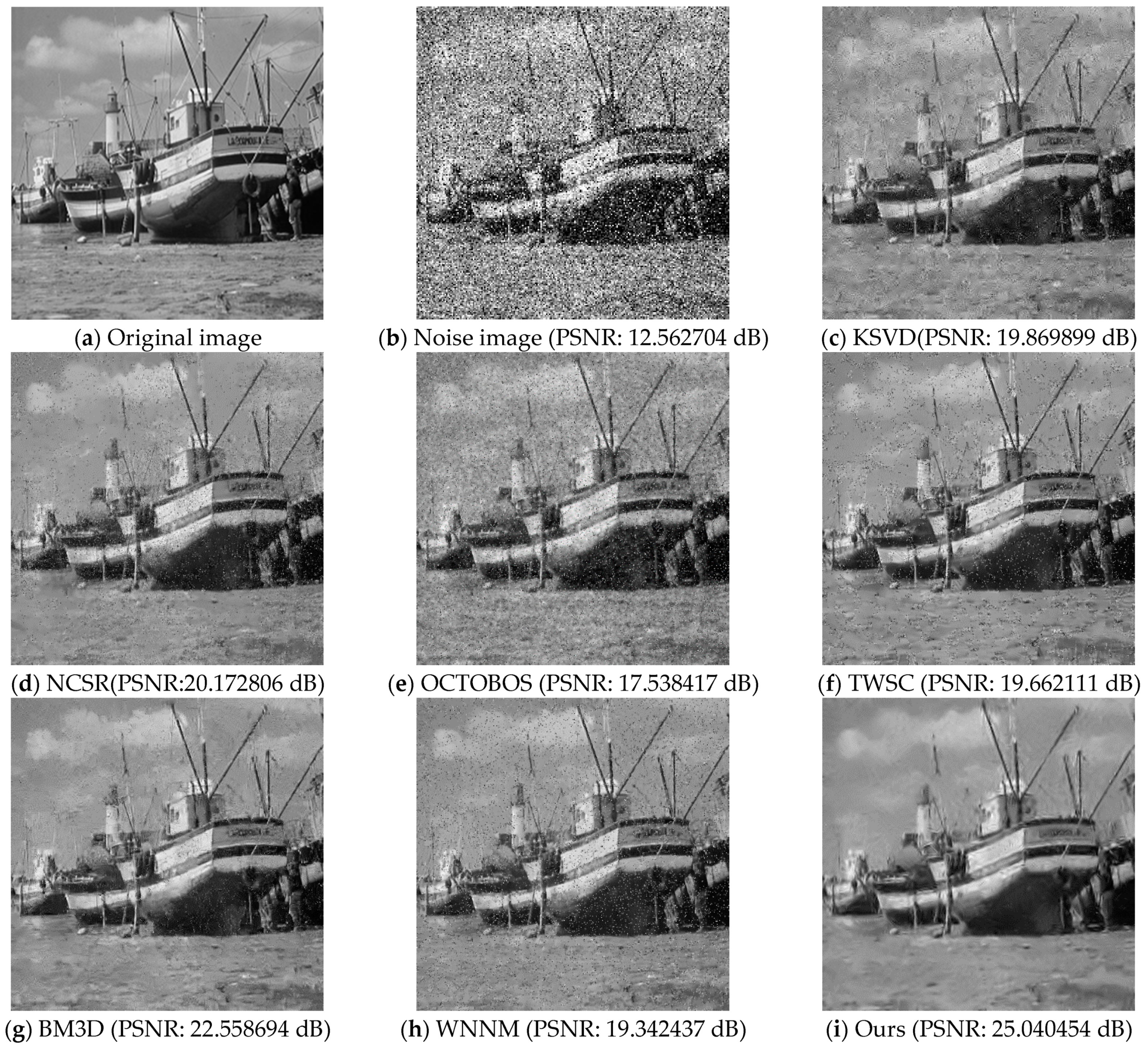
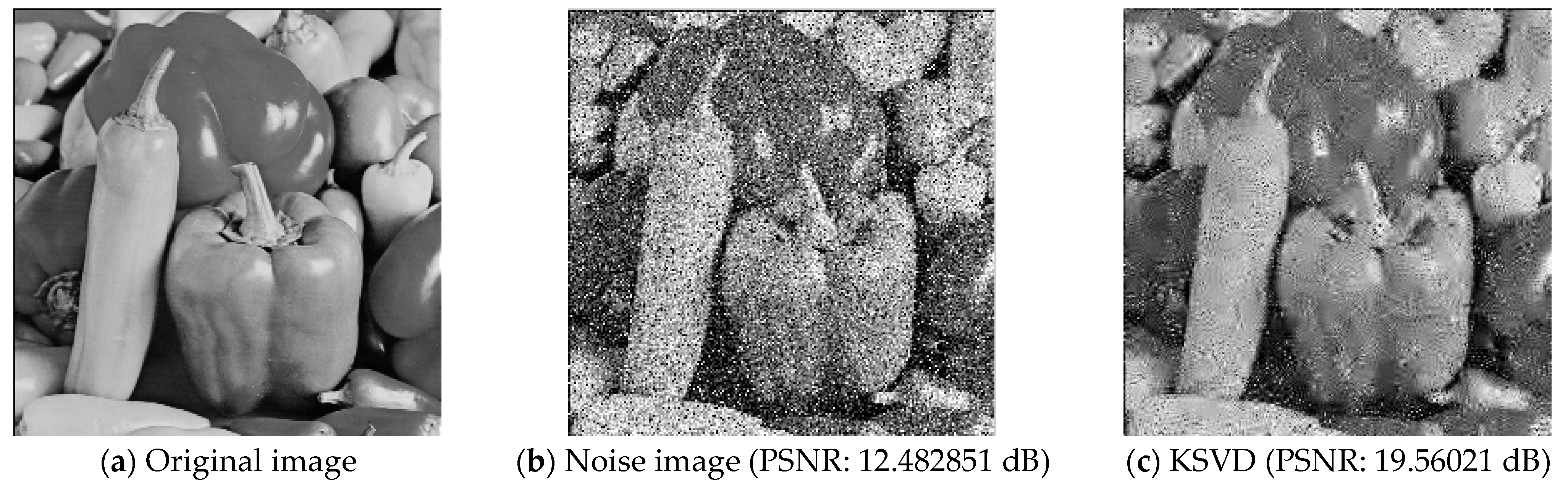
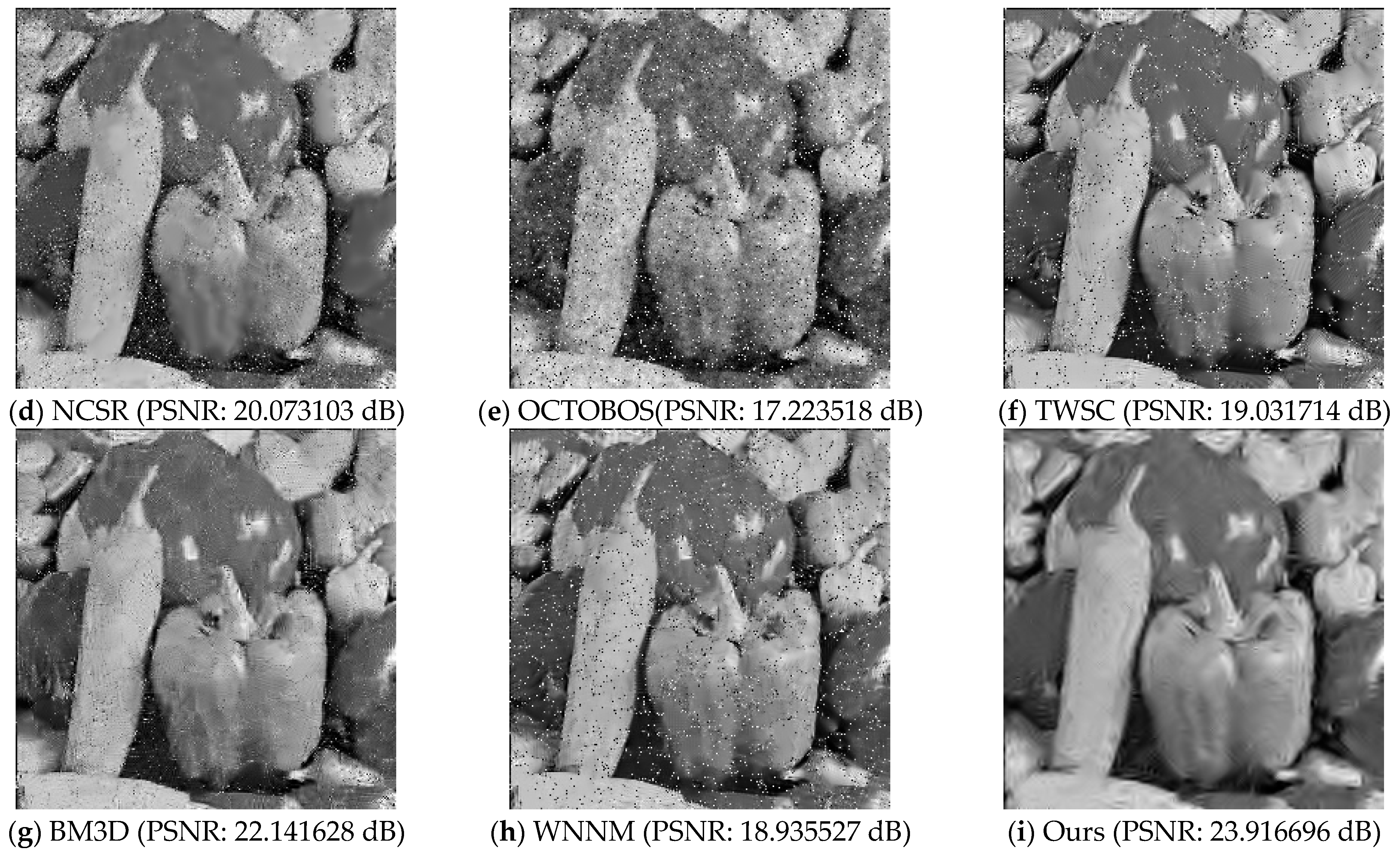
In order to feel the denoising effect of each algorithm on the noise images intuitively, the denoised images of lena, boat, and peppers, when $\rho$/$\sigma$ is 0.09/0.03, were randomly selected for comparison and analysis, and they are shown in Figure 7, Figure 8 and Figure 9. At the same time, Figure 10 shows the line charts of the lena image on PSNR, RMSE, SSIM, and FSIM with different algorithms to help us make further comparison and analysis.

From these denoised images, we can see that, for the mixed noise with salt and pepper + Gaussian noise, several other algorithms, of which KSVD and OCTOBOS are the most prominent, cannot remove the noise cleanly, except for BM3D and our algorithm, and a certain number of spots remain on the image. It also shows that these algorithms have extremely limited ability to remove mixed noise and cannot maintain the effective restoration of image detail information. Moreover, they cannot well retain image edge information. The overall picture of the denoised image is slightly rough. The BM3D algorithm can effectively remove the mixed noise, but it is still insufficient to restore the details of the image. It damages the edge of the image to a certain extent, making the edge part look fuzzy and thus losing more details, which reflects the limited ability of the BM3D algorithm to remove the mixed noise. Relatively speaking, the denoised image of our algorithm is clean. On the premise of ensuring the overall quality of the image, it can successfully remove the mixed noise and can retain the details and edge information of the image more completely. Compared with other algorithms, it has the strongest image restoration ability.

Furthermore, we can find that, from Figure 10, PSNR, SSIM, and FSIM are steadily decreasing and RMSE is steadily increasing with the rise in noise level. The four trend lines are displayed approximately as a straight line with a low slope, which fully illustrates the robustness and stability of our algorithm. However, we still need to point out that, compared with other algorithms, our algorithm has better denoising ability, but when the noise level increases, the denoised images will inevitably show over-smoothness and a reduced ability to restore details, which is what we need to improve on in our future work.

4. Conclusions

This paper proposes a filtering algorithm for mixed noise with salt and pepper + Gaussian noise combined with the improved median filter algorithm, the improved wavelet algorithm, and the improved NLM algorithm. The algorithm makes full use of the advantages of the median filter in removing salt and pepper noise, improving the original median filter algorithm, and utilizing two-level detection to accurately divide the pixel points into signal points and noise points, which can filter salt and pepper noise effectively. In addition, the algorithm also improved the two algorithms by virtue of the good performance of wavelet threshold algorithm and NLM algorithm in filtering Gaussian noise. The improved wavelet threshold algorithm has a more scientific threshold function than the original algorithm; the improved threshold is also more reasonable, and the denoising effect is far better than the hard threshold function and the soft threshold function. The improved NLM algorithm can measure the similarity between image blocks more accurately and match similar image blocks more accurately, for the purpose of achieving a better denoising effect.

Compared with some other algorithms mentioned in this paper, the denoising effect of the proposed algorithm is the best for the mixed noise with salt and pepper + Gaussian noise, the restoration ability of image edge and detail information is the strongest, and the robustness is also the best. However, the denoised images possess the phenomenon of over-smoothness and a weakened ability to restore detail with the increase of noise level. In addition, the experimental images used in this study are standard test images in the field of image processing. How to extend this research to hyperspectral images and achieve real-time processing results in a short time will be an urgent problem that needs to be solved in the next research. At the same time, how to combine this algorithm with the latest research technologies, such as sparse representation and neural networks, to obtain a more stable and better denoising effect is also where we need to make further efforts in future work.