TDGVRPSTW of Fresh Agricultural Products Distribution: Considering Both Economic Cost and Environmental Cost

Abstract

The time-dependent vehicle routing problem of time windows of fresh agricultural products distribution have been studied by considering both economic cost and environmental cost. A calculation method for road travel time across time periods is designed in this study. A freshness measure function of agricultural products and a measure function of carbon emission rate are employed by considering time-varying vehicle speeds, fuel consumptions, carbon emissions, perishable agricultural products, customers’ time windows, and minimum freshness. A time-dependent green vehicle routing problem with soft time windows (TDGVRPSTW) model is formulated. The object of the TDGVRPSTW model is to minimize the sum of economic cost and environmental cost. According to the characteristics of the model, a new variable neighborhood adaptive genetic algorithm is designed, which integrates the global search ability of the genetic algorithm and the local search ability of the variable neighborhood descent algorithm. Finally, the experimental data show that the proposed approaches effectively avoid traffic congestions, reduce total distribution costs, and promote energy conservation and emission reduction.

1. Introduction

In recent years, climate change and carbon emissions have gradually become a common challenge for human society. In the work report of the Chinese government in 2021, carbon peak and carbon neutralization were first mentioned and immediately became the focus of social discussion. According to the CO₂ Emissions from Fuel Combustion: Overview report released by the International Energy Agency in 2020, global carbon dioxide emissions reached a record 33.5 billion tons in 2018, with transport accounting for 24 percent of the total at 8.04 billion tons, while road transport accounted for three-quarters of the total carbon emissions in the transport sector. Therefore, it is of great practical significance to deeply study the green vehicle routing problem and promote energy- saving and emission reduction in the delivery of fresh products.

Previous studies on the green vehicle routing problem (GVRP) can be divided into three categories: vehicle routing problem related to reverse logistics [1], vehicle routing problem related to new energy vehicles, and fuel vehicle routing problem aiming to reduce environmental pollution. The GVRP problem defined in this article refers only to the last one. Bektaş and Laporte [2] proposed the pollution routing problem (PRP) for the first time in 2011. Green vehicle routing problem (GVRP) was first proposed by Erdoğan et al. [3] in 2012. Although the two concepts have different names, they are essentially the same, and this paper defines them both as GVRP. However, relevant studies can be traced back to the relationship between vehicle fuel consumption rate and driving speed proposed by Chang and Morlok in 2005 [4]. Subsequently, many scholars have conducted in-depth research on this issue.

The literature can be divided into three categories based on different objective functions, and the three categories are as follows.

• The first category takes carbon emission or fuel consumption as the optimization target. Aiming to minimize fuel consumption, Suzuki [5] established the pollution routing problem (PRP) model with capacity and vehicle number constraints. Li et al. [6] established a multi-depot vehicle routing problem (MDVRP) model that can share depot resources. Considering that the speed of vehicles on various sections depends on the time of departure and the time period in which the vehicles are travelling, Alinaghian and Naderipour [7] established the time-dependent vehicle routing problems (TDVRP) model and allowed multiple paths to be selected between nodes; aiming to minimize carbon emissions, Manerba et al. [8] used the emission factor model to convert the mileage of vehicles into carbon emissions. Yu et al. [9] constructed the heterogeneous fleet green vehicle routing problem with time windows (HFGVRPTW). Ehmke et al. [10] considered that vehicle speed changed with different time periods and road sections. The vehicle speed was defined as a random variable, and the influence of speed and load on the path to carbon emission minimization was analyzed. A TDVRP model with vehicle numbers constraint was constructed.
• The second type takes environmental cost and economic cost as the optimization target. Micale et al. [11] built models including maximum vehicle capacity, speed, carbon emissions, asymmetric paths, and time windows constraints, and applied the technique for order performance by similarity to ideal solution (TOPSIS) technology to integrate economic and environmental factors. TOPSIS is a criterion for selecting the most suitable solution. Fukasawa et al. [12] took the speed as a continuous decision variable, adopted the road section speed optimization strategy to make vehicles run at the optimal speed in each road section, and took the minimization of the total cost composed of fuel consumption cost and driver’s salary as the optimization objective, respectively, and constructed a PRP model and open green vehicle routing problem with time windows (GVRPTW) model with vehicle numbers and time window constraints. Aiming at the one-to-one pickup and delivery problem, Soysal et al. [13] constructed a heterogeneous VRPTW model with the optimization objective of minimizing the total cost composed of fuel consumption cost, driver wage cost, and penalty cost for violating the time windows, considering that vehicle speed varies with urban and non-urban sections.
• The third category takes two or more conflicting optimization objectives as objective functions. Giallanza and Puma [14] assumed that customer demand was a fuzzy number simulated by a time-dependent algorithm and established a multi-objective fuzzy chance-constrained programming model. Ghannadpour and Zarrabi [K] established a multi-objective heterogeneous VRPTW model with fuel consumption, minimizing vehicle use and maximizing customer satisfaction as optimization objectives. Zulvia et al. [15] constructed a multi-objective GVRPTW model of perishable products, with operating cost, deterioration cost, carbon emission minimization, and customer satisfaction maximization as optimization objectives. Bravo et al. [16] constructed a multi-objective PRPTW model for heterogeneous VRPPD with the optimization objectives of minimizing total fuel consumption and total driving time and maximizing the number of customers served.

In the literature on the vehicle routing problem with time windows, some literature explored the relationship between time windows and pollution emission [17,18,19]. Representative works include the following: Manerba et al. [8] analyzed the impact of two different distribution policies on carbon emissions and proved that the VRPTW model had lower carbon emissions than the DCVRP model at the same time interval through practical cases. However, they used the emission factor model to estimate carbon emissions, and simply converted the distance of vehicles into carbon emissions without considering the impact of vehicle speed, load, slope, and other factors on carbon emissions. Munoz-villamizar et al. [20] proposed an approach using a mixed-integer linear programming model to assess the impact of extended delivery times, using data from real cases to analyze the impact of different extended delivery times on distance traveled, transportation costs, and carbon emissions. Experimental results show that delivery times of up to four days can save 57% of total mileage, 61% of total cost, and 56% of fuel consumption and/or CO₂ emissions. However, the experiment lacked the overall consideration of the three optimization objectives, and its case scale was small, so the method is not suitable for solving large-scale problems. Liu et al. [21] established a TDVRPTW model with the optimization objective of minimizing the sum of driver cost, fuel consumption, and carbon emission, and proposed an improved ant colony algorithm (IACACAA) with a congestion avoidance method to solve the model. Experiments were designed to compare the large time window and the tight time window, proving that cases with short service time and a large time window could obtain vehicle routes with lower total cost and thus reduce carbon emissions.

For the above three types of GVRP models, solving algorithms can be divided into the precise algorithm, traditional heuristic algorithm, and meta-heuristic algorithm. The specific summary is as follows.

• The precise algorithm is one that can find an optimal solution to a problem. Yu et al. [9] proposed an improved branch price algorithm (BAP) to solve HFGVRPTW, and the results showed that the improved BAP algorithm greatly reduces the branch and calculation time. The model established by Xiao and Konak [22] took into account capacity and mileage constraints, time windows constraints, heterogeneous fleets, and time-varying road network conditions and proposed a hybrid algorithm of mixed integer linear programming (MIP) and iterative neighborhood search.
• The basic idea of the traditional heuristic algorithm is to start from the current solution, search for a better solution in the neighborhood of the current solution and continue to search until there is no better solution. Li et al. [23] improved the local search stage of the Clarke and Wright heuristic algorithms to solve the two-echelon position path problem (2E-LRP). In the hybrid heuristic algorithm designed by Wang et al. [24], the Clarke and Wright savings heuristic algorithm (CWSHA) and the sweep algorithm were used to generate the initial population continuously.
• Metaheuristic algorithm is an improvement of the heuristic algorithm, which is the combination of the random algorithm and local search algorithm. Demir et al. [25] proposed an adaptive large-scale neighborhood search algorithm based on simulated annealing. Eight removal operators and four insertion operators were used to search the neighborhood to generate a new solution and simulated annealing acceptance rules were used to determine whether to select the new solution as the current solution. Sadati et al. [26] developed a hybrid general variable neighborhood search and tabu search approach to solve the model effectively.

Population-based metaheuristics have good global searching ability and can carry out distributed computation conveniently and speed up the solving speed by using inherent parallelism. The latest multi-point heuristic algorithm includes the quantum evolutionary algorithm (QEA) [27], quantum inspired differential evolution algorithm (QDE) [28], improved differential evolution (DE) algorithm [29], etc. However, the local searching ability of the multi-point heuristic algorithm is poor, and the searching efficiency is low in the later stage of calculation. In recent studies, many scholars at home and abroad combine various meta-heuristic algorithms together to form a hybrid meta-heuristic algorithm and make substantial improvements on the basis of some basic algorithms so that the efficiency of the algorithm is greatly improved, and there are abundant achievements in this aspect. This paper designs the algorithm based on the above research results.

In particular, this paper focuses on a certain type of GVRP, i.e., the GVRP of fresh agricultural products. There are relatively few previous studies on GVRP of fresh agricultural products. Zulvia [15] consider the GVRP model of perishable products with operational costs, deterioration costs, carbon emissions, and customer satisfaction as optimization targets, and the objective gradient evolution algorithm was used to solve the model. Rahbari et al. [30] presented a bi-objective mixed integer linear programming (MILP) model for the vehicle routing and scheduling problem with cross-docking for perishable products. Alkaabneh et al. [31] considered the inventory routing problem for perishable products and aimed at maximizing supplier profits and minimizing the cost of fuel consumption, inventory retention, and greenhouse gas emissions, and they developed a precise method based on Bender decomposition to find high-quality solutions in a reasonable time. However, these studies did not focus on the impact of time sensitivity of different fresh agricultural products on distribution planning. At the same time, under different optimization objectives the proportion of freshness loss cost and carbon emission cost to the total cost has not been proven.

The model formulated in this paper belongs to the second type of GVRP model, and the algorithm adopted is a hybrid meta-heuristic algorithm. In this paper, a time-dependent green vehicle routing problem with soft time windows (TDGVRPSTW) for fresh products distribution is established. The TDGVRPSTW problem is an extension of the traditional GVRP model, which adds time-dependent road network conditions and soft time windows. Time-dependent means that the speed of a vehicle on each road section is related to its time period, and the speed is different in different time periods. Adding time-dependent conditions to the model can make the model closer to reality. The soft time windows are relative to the traditional hard time windows. In the soft time windows model, the time when the vehicle arrives at the customer is not strictly limited. The vehicle can start service at any time when it arrives at the customer, but it needs to pay a penalty cost to start service outside the service time windows. A hybrid algorithm combining the genetic algorithm and variable neighborhood descent algorithm is used to solve the model. It also analyzes the relationship between distribution economic cost and environmental cost, hoping to provide fresh products and a decision-making reference for distribution.

The innovations and contributions of this paper are described as follows.

• A hybrid algorithm combining adaptive genetic algorithm and neighborhood search algorithm is designed, which considers both the search breadth and the search depth. The chromosomes in the population are disturbed by the crossover and mutation operation of the genetic algorithm, and the excellent chromosomes in the population are deeply searched by the neighborhood search algorithm.
• Different fresh agricultural products have different perishability. Does the difference in perishability of fresh agricultural products have an impact on driving routes and customer assignment schemes? This paper will clarify the problem through experiments.
• In order to improve the quality and diversity of the initial population, three different methods were used to generate the initial population in this paper. The three methods are, respectively, the CW saving algorithm, nearest neighbor insertion algorithm, and random method.

The remainder of this paper is organized as follows. In Section 2, we give a detailed description of the TDGVRPSTW model formulated in this paper. Section 3 presents the proposed variable neighborhood adaptive genetic algorithm. Experimental results and analyses are given in Section 4. Finally, conclusions are given in Section 5.

2. Problem Description and Model Formulation

2.1. Problem Description

A distribution center distributes fresh agricultural products to customers. The customer location, demand, time window, and service time are known. The vehicle can start serving the customer before or after the time window, but the vehicle has to pay a penalty cost. Vehicles have a fixed cost, driving cost, penalty cost, and carbon emission cost. Fresh products will produce a freshness loss cost over time. The total cost as the optimization objective includes vehicle transportation cost, vehicle fixed use cost, time window penalty cost, carbon emission cost, and freshness loss cost. Decision problem: how do we make a distribution plan to minimize the total cost?

The following assumptions are made:

• The vehicle is of the same type and the driving speed is different in different time periods at the same time, and you can start at different times and return to the distribution center after completing the task;
• The customer demand is less than the vehicle capacity, and there is only one vehicle for its services;
• The distribution center has a time window within which vehicles must leave and return;
• The engine is switched off while the vehicle is waiting and during customer service, and there is no fuel consumption or carbon emission.

2.2. Model Formulation

2.2.1. Calculation Method of Travel Time for the Cross Time Section

A driving time calculation method was designed based on time division. The working time of the distribution center is divided into multiple time periods, and the vehicle driving speed is different in different time periods. Let $F$ be the length of the period;$H=\left\{H_0,H_1,\cdots ,H_L\right\}$ is a set of all time, $\left[H_{h-1},H_h\right]$ is the $h-th$ period. The driving speed of vehicles in different time periods is shown in Figure 1. $d_{ijk}^h$, $t_{ijk}^h$ and $g_{ijk}^h$ respectively represent the distance, time, and speed of vehicle $k$ on the road section $\left(i,j\right)$ within the time period $h$; $D_{ij}$ is the distance of the road section $\left(i,j\right)$; $D_{ij}^h$ is the distance of vehicle $k$ finishing $\left(i,j\right)$ remaining distance after time $h$; $L_{ik}$ is the point in time when vehicle $k$ leaves customer $i$; $h_k$ is the remaining drivable time of vehicle $k$ within the time period $h$, then the calculation steps of vehicle $k$’s driving time $t_{ijk}$ on the road section $\left(i,j\right)$ are as follows:

• Calculate the travel time in the initial period.$d_{ijk}^h=g_{ijk}^h{h}_k$. If $d_{ijk}^h\ge D_{ij}$, then $t_{ijk}^h=D_{ij}/g_{ijk}^h$, $t_{ijk}=t_{ijk}^h$, end of calculation; If $d_{ijk}^h<D_{ij}$, $D_{ij}^h=D_{ij}-d_{ijk}^h$, $t_{ijk}^h=h_k$, turn to step 2.
• $\zeta =1$; $d_{ijk}^{h+\zeta }=g_{ijk}^{h+\zeta }F$, if $d_{ijk}^{h+\zeta }<D_{ij}^{h+\zeta -1}$, then $t_{ijk}^{h+\zeta }=F$, $D_{ij}^{h+\zeta }=D_{ij}^{h+\zeta -1}-d_{ijk}^{h+\zeta }$, repeat step 2; otherwise, $t_{ijk}^{h+\zeta }=D_{ij}^{h+\zeta -1}/g_{ijk}^{h+\zeta }$, $t_{ijk}={\displaystyle \sum _{h\in H}}{t}_{ijk}^h$, the calculation of the driving time of section $\left(i,j\right)$ is completed.

Figure 1. Vehicle speed in different time periods.

Figure 1. Vehicle speed in different time periods.

2.2.2. Freshness Loss Coefficient Function

The freshness loss coefficient in the literature [32] was used to measure the freshness loss of fresh products: ${\xi }_{0i}={\left(T_{is}/T\right)}^r$, where $T$ is the shelf life of agricultural products and the time when customers receive fresh products $T_{is}\le T$, $rϵ\left(0,1\right)$ is the time-sensitive adjustment factor. Different fresh products have different values, and the smaller the $r$ value, the more sensitive the agricultural products are to time.

2.2.3. Carbon Emission Estimation Function

In order to quantitatively study the calculation of carbon emissions, this paper refers to the carbon emission estimation model in reference [33]. The carbon emission estimation function of freight cars with vehicle weight between 3.5 t and 40 t is:

$${\epsilon }^h\left(v\right)=a_0+a_{1}v+a_2{v}^2+a_3{v}^3+\frac{a_4}{v}+\frac{a_5}{v^2}+\frac{a_6}{v^3}$$

(1)

where ${\epsilon }^h\left(v\right)$ is the carbon emission rate (g/km) of the vehicle when it is empty and running on the road with slope of 0, $v$ is the average speed of the vehicle (km/h), and the value of parameter $\left(a_0,a_1,a_2,a_3,a_4,a_5,a_6\right)$ is related to the weight range of the vehicle.

Load correction function is:

$${\lambda }^h\left(v,\phi \right)=b_0+b_1\phi +b_2{\phi }^2+b_3{\phi }^3+b_{4}v+b_5{v}^2+b_6{v}^3+\frac{b_7}{v}$$

(2)

where $\phi$ is the ratio of the actual load of the vehicle to its capacity, $\nu$ is vehicle speed (km/h), the parameter $b$ for the correction coefficient of load, the value is related to the weight range of the vehicle. If the driving distance of vehicle $k$ in time period $h$ is $d^h{}_{ijk}$ (km), the calculation formula of its carbon emission $E^h{}_{ijk}$ (kg) is shown as follows:

$$E^h{}_{ijk}={\epsilon }^h·{\lambda }^h·\frac{d^h{}_{ijk}}{1000}$$

(3)

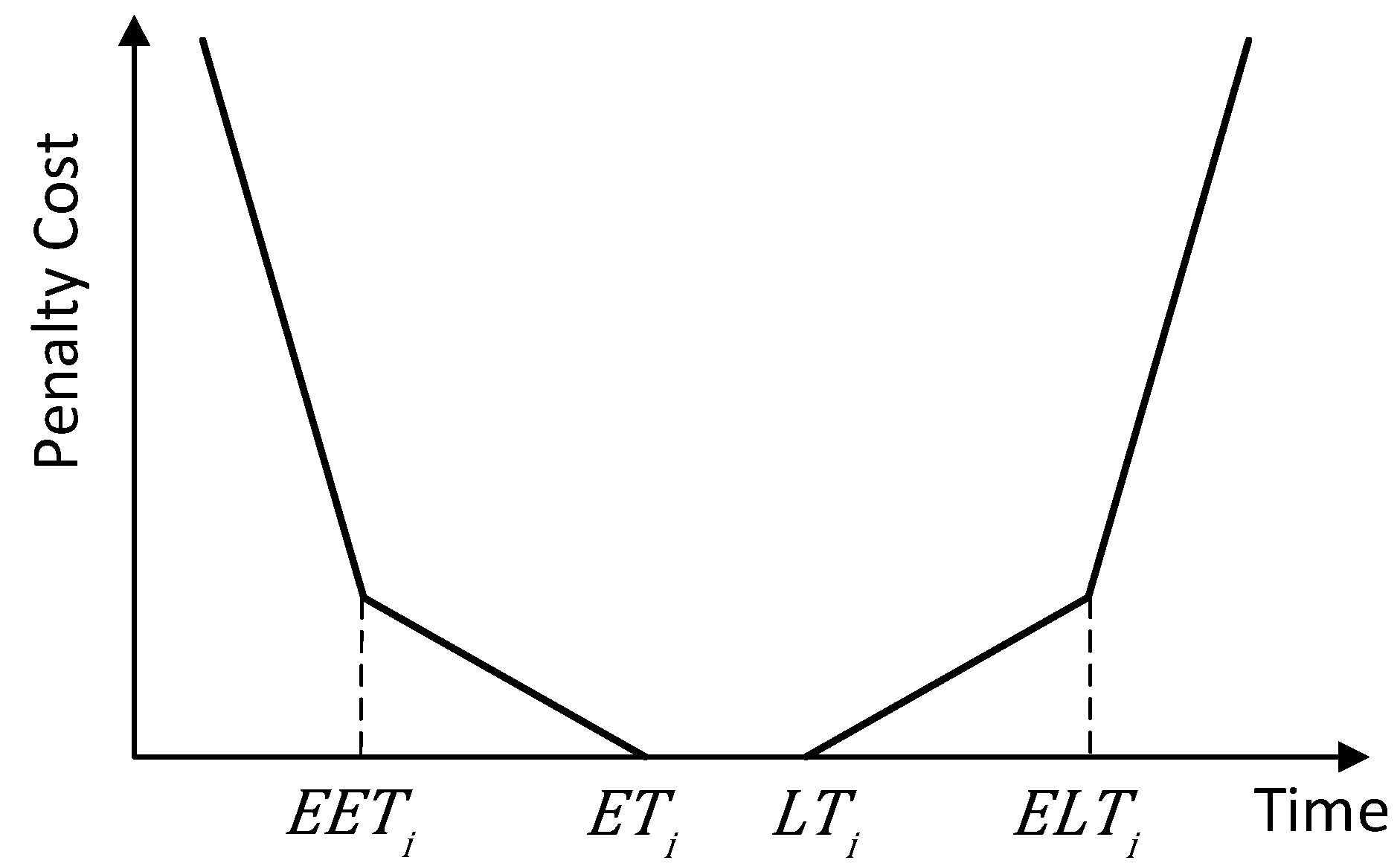
2.2.4. Soft Time Windows Model

Compared with the traditional hard time windows, soft time windows have many advantages [34]. For example, if the time window is set as soft, the number of vehicles used and the total mileage of vehicles can be greatly saved; the soft time windows model is more general and contains the requirements of hard time windows, so the algorithm designed for solving soft time window models can be used to solve the problem with hard time windows by appropriately increasing the penalty value when deviating from the time windows. In some cases, there may be no feasible solution according to the requirements of hard time windows, but there is always a feasible solution according to the requirements of soft time windows.

The broken line soft time windows model was proposed by Han et al. [35]. The broken line soft time window adds a period that can be tolerated by customers based on the ordinary soft time window. The penalty cost curve is shown in Figure 2. The period $\left[E{T}_i,L{T}_i\right]$ is the optimal time window, and no penalty cost is needed to start the service within this period. When the vehicle starts service in $\left[EE{T}_i,E{T}_i\right]$ or $\left[L{T}_i,EL{T}_i\right]$, there is less penalty cost; if the service start time is not within the range of $\left[EE{T}_i,EL{T}_i\right]$, a high penalty cost is required. Limits of time points that the customer can tolerate can be determined by$EE{T}_i=E{T}_i-\theta s_i$,$EL{T}_i=L{T}_i+\theta s_i$, where $\theta$ is the customer tolerance coefficient and $s_i$ is the service time of customer $i$.

The penalty cost function under the broken line soft time windows is as follows:

$$P_c\left(T_{ik}\right)=\{\begin{array}{cc}{p}_1\left(EE{T}_i-T_{is}\right)+p_2\left(E{T}_i-EE{T}_i\right),\hfill & \hfill T_{is}\le EE{T}_i\\ p_2\left(E{T}_i-T_{is}\right),\hfill & \hfill EE{T}_i<T_{is}\le E{T}_i\\ 0,\hfill & \hfill E{T}_i<T_{is}\le L{T}_i \\ p_3\left(T_{is}-L{T}_i\right),\hfill & \hfill L{T}_i<T_{is}\le EL{T}_i\\ p_3\left(EL{T}_i-L{T}_i\right)+p_4\left(T_{is}-EL{T}_i\right),\hfill & \hfill EL{T}_i<T_{is}\end{array}$$

(4)

where $p_1,p_2,p_3,p_4$ are penalty costs per unit of time in the corresponding period, respectively.

2.2.5. Symbol and Variable Definitions

$N$ is the set of all nodes in the distribution network, including the distribution center and all customer points;

$N^{\prime }=N\backslash \left\{0\right\}$ is the set of all customer points;

$K$ is the collection of vehicle serial numbers;

$H$ is the set of all time periods;

$D_{ij}$ denotes the distance between nodes $i,j$;

$\phi$ is the vehicle unit distance driving cost;

$\delta$ is the fixed use cost of the vehicle;

$T_{ik}$ is the time when the vehicle $K$ arrives at the customer $i$;

$T_{is}$ refers to the time when the vehicle starts to serve customer $i$ and the time when the customer receives fresh products;

$P_c\left(T_{ik}\right)$ is the penalty cost function of the time window;

$E_{ijk}^h$ is the carbon emission (kg) of vehicle $k$ on the road section $\left(i,j\right)$ in the period $h$;

$\mu$ represents unit carbon emission cost (yuan /kg);

${\xi }_{0j}$ indicates freshness loss coefficient;

$p$ is the price of fresh products (yuan/kg);

$q_j$ represents the demand (kg) of customer $j$;

$Q$ represents the demand of all customers in the distribution network;

$t_{ijk}^h$ represents the time for vehicle $k$ to travel on section $\left(i,j\right)$ within the period $h$;

$d_{ij}^h$ represents the distance traveled by vehicle $k$ on the road section $\left(i,j\right)$ within the time period $h$; $s_i$ indicates the service duration for customer $i$.

$t_{ijk}$ represents the total time for vehicle $k$ to travel on section $\left(i,j\right)$;

$L_{ik}$ is the point in time when vehicle $k$ leaves customer $i$;

$X_{ijk}$ is a variable of 0–1. $X_{ijk}=1$ when the vehicle $k$ travels on the section $\left(i,j\right)$, otherwise $X_{ijk}=0$;

$x_{ijk}^h$ is a variable of 0–1. $x_{ijk}^h=1$ when the vehicle $k$ travels on the road section $\left(i,j\right)$ within the time period $h$, otherwise $x_{ijk}^h=0$;

$y_{ik}$ is a variable of 0–1. When vehicle $k$ visits customer $i$, $y_{ik}=1$; otherwise, $y_{ik}=0$;

$z_k$ is a 0–1 variable, if vehicle $k$ is used $z_k=1$, otherwise $z_k=0$.

2.2.6. TDGVRPSTW Model Formulation

The TDGVRPSTW model is built as follows:

$$minC=C_1+C_2+C_3$$

(5)

Among them

$$C_1={\displaystyle \sum _{i\in N}{\displaystyle \sum _{j\in N}{\displaystyle \sum _{k\in K}{X}_{ijk}{D}_{ij}\phi }}}+{\displaystyle \sum _{k\in K}{z}_k\delta }+{\displaystyle \sum _{i\in N^{\prime }}{P}_c\left(T_{ik}\right)}$$

$$C_2={\displaystyle \sum _{h\in H}{\displaystyle \sum _{i\in N}{\displaystyle \sum _{j\in N}{\displaystyle \sum _{k\in K}{x}_{ijk}^h{E}_{ijk}^h\mu }}}}$$

$$C_3={\displaystyle \sum _{k\in K}{\displaystyle \sum _{j\in N^{\prime }}{\xi }_{0j}p{q}_j{y}_{jk}}}$$

Subject to:

$${\displaystyle \sum _{i\in N^{\prime }}{q}_i{y}_{ik}\le Q},\forall k\in K$$

(6)

$${\displaystyle \sum _{j\in N^{\prime }}{X}_{0jk}\le 1,\forall k\in K}$$

(7)

$${\displaystyle \sum _{k\in K}{y}_{ik}}=1,\forall i\in N^{\prime }$$

(8)

$${\displaystyle \sum _{i\in N}{X}_{ijk}}={\displaystyle \sum _{j\in N}{X}_{ijk}},\forall k\in K$$

(9)

$$t_{ijk}={\displaystyle \sum _{h\in H}{X}_{ijk}{t}_{ijk}^h,\forall i\in N,j\in N,k\in K}$$

(10)

$$D_{ij}={\displaystyle \sum _{h\in H}{d}_{ijk}^h{X}_{ijk}},\forall i\in N,j\in N,k\in K$$

(11)

$$E{T}_0\le X_{i0k}\left(T_{is}+s_i+t_{i0k}\right)\le L{T}_0,\forall i\in N^{\prime },k\in K$$

(12)

$$T_{is}\ge T_{ik},\forall i\in N^{\prime },k\in K$$

(13)

$$L_{ik}=T_{is}+s_i,\forall i\in N,j\in N,k\in K$$

(14)

$$t_{0i}=T_{is},\forall i\in N^{\prime },k\in K$$

(15)

$${\displaystyle \sum _{j\in N^{\prime }}{X}_{0jk}\le 1},\forall k\in K$$

(16)

$$x_{ijk}^h\in \left\{0,1\right\},X_{ijk}\in \left\{0,1\right\},y_{ik}\in \left\{0,1\right\},z_k\in \left\{0,1\right\}$$

(17)

Equation (5) of the objective function represents cost minimization, where $C_1$ represents distribution cost, including vehicle transportation cost, vehicle fixed use cost, and soft time window penalty cost. The time windows penalty cost is defined in Equation (4). $C_2$ represents the cost of carbon emission and $C_3$ represents the cost of freshness loss. Carbon emission cost is defined in Equation (3), and freshness loss cost is defined in Section 2.2.2. Equation (6) represents the load limit of each vehicle. Equation (7) indicates that each car can only be used once. Equation (8) indicates that each customer must be served only once. Equation (9) indicates that the number of departing and arriving vehicles at each node should be balanced. Equation (10) represents the relationship between the road section driving time and the vehicle driving time within the time period. Equation (11) represents the relationship between the road section distance and the distance traveled by the vehicle in each period. Equation (12) indicates that vehicles returning to the distribution center should meet the constraints of the distribution center’s working time window. Equation (13) represents the relationship between the start time of service and the arrival time. Equation (14) represents the relationship between the service start time, duration, and departure time. Equation (15) indicates the time when the customer receives the fresh products. Equation (16) indicates that the customer’s demand is less than the vehicle capacity, and there is only one vehicle to serve them. Equation (17) represents the variable value constraint.

3. Variable Neighborhood Adaptive Genetic Algorithm

3.1. Algorithm Model

The adaptive genetic algorithm (AGA), compared with simple genetic algorithm, has the advantages of fast convergence and superior optimization ability. The variable neighborhood descent algorithm (VND) can combine with other heuristic rules for effective local search. Based on the advantages of the two algorithms, a variable neighborhood adaptive genetic algorithm (VNAGA) is designed to solve the TDGVRPSTW model in this paper. The algorithm solving process is shown in Figure 3.

3.2. Initial Population

The chromosomes adopt the form of natural number coding, with the natural numbers from $1~n$ representing the customer nodes. Each chromosome is an arrangement of natural numbers with equal length. When the chromosome is decoded into vehicle paths, the path segments are divided according to the vehicle load and the latest operation time of the distribution center. In order to ensure the diversity of the population, this paper uses the Clarke–Wright saving algorithm (CW saving algorithm), nearest neighbor insertion method, and random method to generate the initial population. In order to take into account the quality and diversity of chromosomes at the same time, the number of chromosomes generated by different methods is allocated according to the following rules: first, a chromosome is generated by the CW saving algorithm, and the chromosome is copied $n{o}_s$ times into the population, where $n{o}_s$ is a random integer between $\left[1, 0.5popsize\right]$. Next, the nearest neighbor insertion method is used to generate the number of $\left(0.5popsize\right)-n{o}_s$chromosomes and adds them to the population. Finally, the random method generates the number of $0.5popsize$ solutions to complete the initialization of the population. The specific operation steps of each part are as follows.

Firstly, the improved CW saving algorithm [36] is adopted. Since in the estimation function of carbon emissions the deadweight will impact carbon emissions, it is helpful to place the nodes with large demand in the first part of the route to reduce the overall carbon emissions. Accordingly, this paper considers the deadweight based on the traditional saving algorithm, and the formula for calculating the amount of saving is $S\left(i,j\right)=D_{0i}+D_{0j}-D_{ij}+\gamma \left(q_i+q_j\right)$, where $\gamma$ is the load factor. See Figure 4a for the specific steps. The route constraint in the Figure 4 refers to the vehicle load limit and the latest time limit for returning to the distribution center, while the global constraint in the figure refers to the vehicle number limit and node number limit.

The second method to generate the initial population is the nearest neighbor insertion algorithm [37]: the formula for calculating the insertion value is $B\left(i,j\right)={\sigma }_1{D}_{ij}+{\sigma }_2\left(T_{js}-L_{ik}\right)+{\sigma }_3\left(L{T}_j-T_{jk}\right)$, where $\left(T_{js}-L_{ik}\right)$ is the difference between the time when node $j$ starts service and the time when node $i$ completes service and is used to represent the proximity degree of nodes $i,j$ in time. $\left(L{T}_j-T_{jk}\right)$ is the difference between the lower limit of the optimal service time window of node $j$ and the time point of reaching node $j$, which is used to represent the tension degree of the time window. The weight is ${\sigma }_1+{\sigma }_2+{\sigma }_3=1$, and ${\sigma }_1,{\sigma }_2,{\sigma }_3>0$. See Figure 4b for specific calculation steps.

3.3. Fitness Function

The traditional fitness function is in the form of $f_n=1/c_n$. When using this form of the fitness function, if the fitness value difference of each chromosome is not obvious, the probability of each chromosome being selected is not different, which may lead to mediocre chromosomes being selected into the next generation and excellent chromosomes being eliminated. In order to reduce this situation as much as possible, this paper adopts the principle of pressure, using $f_n=\alpha \left\{max\left(c_n\right)\right\}-c_n$ to express the fitness function, where $c_n$ represents the objective function value of the current chromosome, $max\left(c_n\right)$ represents the maximum objective function value of the current population, and $\alpha$ is a constant greater than 1. This function can increase the difference between the fitness of each chromosome.

3.4. Genetic Operators

3.4.1. Selection Operator

In this paper, the optimal protection strategy and roulette selection method were used to select chromosomes. The specific steps of the optimal protection strategy were to find out the two chromosomes with the highest fitness and the lowest fitness in the current population; the fitness value of the chromosome with the highest fitness was compared with the highest fitness value of each generation in history. If the current value was high, it was regarded as the best-protected chromosome; otherwise, the best-protected object remained unchanged, and it was still the best one in history. The chromosome with the worst fitness value in the current population was replaced by the one with the best protection. In roulette, the probability of each chromosome being selected is $p_n=f_n/({\displaystyle \sum _n}{f}_n)$. The greater the fitness of the chromosome, the more likely it is to be selected for cross-mutation operation.

3.4.2. Crossover Operator

In this paper, we improved the crossover method. Firstly, two crossover gene points $(A$ and $B$) were generated randomly on the paternal chromosomes and divided into two paternal chromosomes in the first segment, middle segment, and the third segment. The middle segment of chromosome $A$ and chromosome $B$ were removed and placed on the first segment of chromosome $B_1$ and the third segment of chromosome $A_1$, respectively. The remaining first and third segments of the parent chromosomes $A$ and $B$ were spliced to the back of the first segment of chromosome $B_1$ and the front of the third segment of chromosome $A_1$, respectively. The genes in the two intersecting segments were kept unchanged in the two offspring chromosomes, and the genes that were duplicated in the intersecting segments in the remaining locations were eliminated. The specific crossover process is shown in Figure 5a. This method integrates the number of iterations, the fitness values of chromosomes and population, and the number of unchanged chromosomes in each generation of population, as shown in Formula (18).

$$P_c=\{\begin{array}{l}{P}_{c1}-\frac{\left(P_{c1}-P_{c2}\right)\left(f_l-f_{avg}\right)}{\left(f_{\max }-f_{avg}\right)\left[1+\exp \left(\frac{-gen\times U}{M\times popsize}\right)\right]},f_l\ge f_{avg}\\ P_{c1}{}^{\left[1+\exp \left(\frac{-gen\times U}{M\times S}\right)\right]}, f_l<f_{avg}\end{array}$$

(18)

In this function, $p_c$ represents the adaptive crossover probability, $p_{c1}$ and $p_{c2}$ are adaptive adjustment parameters, $p_{c1}>p_{c2}$, $f_l$ represents the fitness value of individuals with greater fitness in the chromosomes to be crossed, $f_{avg}$ represents the average fitness value in each generation of the population, and $f_{max}$ represents the maximum fitness value in each generation of the population. $gen$ represents the current number of iterations, $M$ represents the maximum number of iterations, $U$ represents the number of individuals with unchanged chromosomes, and $popsize$ represents the population size.

3.4.3. Mutation Operator

In this paper, the mutation method of randomly exchanging gene positions is adopted. The specific steps are as follows: first, select the chromosome to undergo the mutation operation, and randomly select any two gene positions on the chromosome; an entirely new chromosome is created by swapping genes at the location of the two genes. The mutation process is shown in Figure 5b. The adaptive function of mutation probability is shown as follows:

$$P_m=\{\begin{array}{l}{P}_{m1}-\frac{\left(P_{m1}-P_{m2}\right)\left(f_{\max }-f\right)}{\left(f_{\max }-f_{avg}\right)\left[1+\exp \left(\frac{gen\times U}{M\times popsize}\right)\right]},f\ge f_{avg}\\ P_{m1}{}^{\left[1+\exp \left(\frac{gen\times U}{M\times S}\right)\right]} ,f<f_{avg}\end{array}$$

(19)

$p_m$ represents adaptive mutation probability, $p_{m1}$ and $p_{m2}$ are adaptive adjustment parameters, and $p_{m1}>p_{m2}$, $f$ is the fitness value of the chromosome to be mutated.

3.5. Variable Neighborhood Descent Operator

The operation objects of variable neighborhood descent are the excellent chromosomes in the population. The chromosomes in the population are sorted in order of fitness from high to low, and the chromosomes ranked in the first half are the excellent chromosomes. In each neighborhood search operator, a node is randomly selected first, and then the distance between this node and all other nodes is calculated. The other nodes are arranged in ascending order to form a list of distance values.

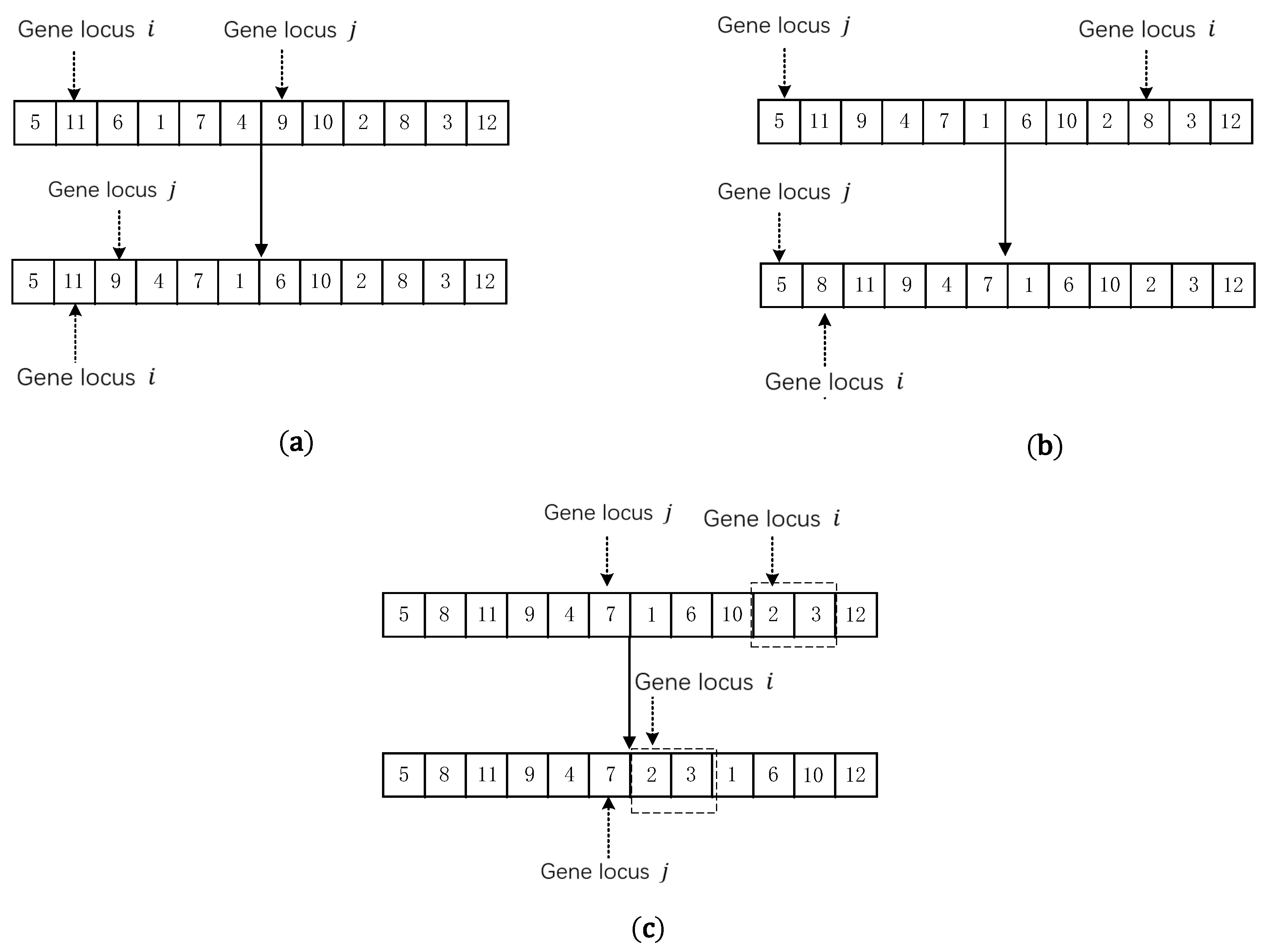
3.5.1. Gene Fragment Inversion Operator

A gene site $i$ was randomly selected on the chromosome. Select a node from the distance value list of node $i$ in order as gene position $j$; a gene fragment is formed between $i$ and $j$ (including $j$ but not including$i$) on the chromosome. The gene fragment is taken out, reversed, and inserted back into the original position of the chromosome, so that $i$ and $j$ are adjacent. If fitness is improved, this operation is retained; otherwise, this operation is repeated until better chromosomes are found, or the maximum number of searches is reached, as shown in Figure 6a.

3.5.2. Insertion Operator of Single Gene Location

A gene site $i$ is randomly taken from the chromosome; gene locus $j$ is selected sequentially from the distance value list of gene locus $i$. The gene locus $i$ is inserted after the gene locus $j$, so that $i$ is adjacent to $j$. The fitness value of the inserted chromosome is calculated. If the fitness is improved, the operation is retained; otherwise, the operation is repeated until a better chromosome is found or the maximum number of searches is reached, as shown in Figure 6b.

3.5.3. Insertion Operator of Double Gene Location

Two adjacent nodes in the chromosome are randomly selected, and the node in front is node $i$. Select node $j$ in the distance value list of node $i$ to insert the two adjacent nodes behind node $j$, making $i$ and $j$ adjacent. The changes of fitness of chromosomes before and after insertion were compared. If the fitness was improved, the operation was retained; otherwise, the operation was repeated until better chromosomes were found or the maximum search times were reached, as shown in Figure 6c.

4. Computational Experiments and Analyses

4.1. Data and Parameter Setting

This paper used part of the data in the Solomn [37] standard sample data set for experiments. These experiments were implemented using Python3.8 programming. After repeated tests, the setting of the relevant parameters of the algorithm was related to the size of the data set used in the experiment, as follows: $p_{c1}=0.7$, $p_{c2}=0.5$, $p_{m1}=0.01$, $p_{m2}=0.008$, maximum iteration number $maxit=100~300$, population $popsize=100~200$, maximum field search times $S_t=15~30$. The weights of the nearest neighbor insertion method were set as follows: ${\sigma }_1=0.4$, ${\sigma }_2=0.4$, ${\sigma }_3=0.2$. In order to get close to the real traffic situation, relevant parameters of the time-varying road network were set as follows: the time of 0 in the distribution center is 7:00 a.m., the traffic jam period is 7:30–9:00 and 17:30–19:00, and the speed is 20 km/h. The setting of vehicle speed refers to the research of Xiao et al. [22], with settings as follows: for the time period $h$, according to the remainder function $\eta =h mod 3$, when $\eta$ is set to (1,2,0), it corresponds to (54,72,42) km/h, respectively, with three time-varying velocities. In the CW saving algorithm, the load factor $\gamma =1$. Time window-related parameters [35] are: $\theta =0.5$, $p_1=1$, $p_2=0.5$, $p_3=1.5$, $p_4=2$, $\phi =8$, $\delta =60$. Referring to Xiao et al. [22], the correlation coefficient of carbon emission model is shown below: $a_0=110$, $a_1=0$, $a_2=0$, $a_3=0.000375$, $a_4=8702$, $a_5=0$, $a_6=0$, $b_0=1.27$, $b_1=0.0614$, $b_2=0$, $b_3=-0.0011$, $b_4=-0.00235$, $b_5=0$, $b_6=0$, $b_7=-1.33$. Fresh products price $p=5$ yuan /kg, shelf life $T=36$ h, regulatory factor $r=0.3$. The unit price of carbon emission is set at $\mu =0.0528$ yuan /kg according to the trading price of Beijing carbon emission market on 30 April 2021, and all the experiments were repeated ten times to get the best result.

4.2. Algorithm Comparison Experiment in VRPSTW Model

In order to verify the effectiveness of the proposed algorithm in the broken line soft time window model, the R101 data set was used in this experiment. One distribution center and the first 25 customers were selected from the data set for validation. The maximum number of vehicles is 25, and the vehicle load capacity is 200 units. As there is minimal literature on vehicle routing problems with broken line soft time window under time-varying road network conditions, there are no studies that can be directly compared; this experiment refers to the broken line soft time windows model of Han et al. [35] to verify and analyze the algorithm. Aiming to minimize the total cost of transportation and distribution, Han et al. [35] constructed a general mathematical model for VRP with flexible time windows. Meanwhile, a commonality hyper-heuristic genetic algorithm was presented. The algorithm uses genetic algorithm as the upper search algorithm and three heuristic algorithms as the underlying search rules, and optimizes the algorithm by pre-sorting, local search, and global optimization. The difference between this model and this paper is that the vehicle speed is fixed, and the objective function only includes the $C_1$ part of the objective function in this paper. Therefore, to make a comparison, the distance and time between different nodes are set in this experiment to be converted into the same unit, which is consistent with the literature and has the same objective function. The other parameters remain the same.

The comparison between the optimal solution obtained by the algorithm and the reference literature is shown in

Table 1. Comparison of experimental results in VRPSTW model.

Variable Neighborhood Adaptive Genetic Algorithm						Hyper-Heuristic Genetic Algorithm
TC	IT	VN	VR	LR/%	RT	TC	IT	VN	VR	LR/%	RT
4627.1	14	4	0-11-19-7-10-20-9-1-0	42.5	229.41	4763.8	38	4	0-5-16-6-18-8-17-13-0	47.0	220.25
			0-14-15-2-22-23-25-4-0	53.5	223.0				0-14-15-2-22-23-4-25-0	53.5	212.74
			0-21-12-3-24-0	23.0	190.0				0-21-12-3-24-1-0	28.0	221.02
			0-5-16-6-18-8-17-13-0	47.0	221.26				0-11-19-7-10-20-9-0	37.5	218.40

, where TC represents the total cost (unit: yuan), IT represents number of iterations, VN represents the number of vehicles, VR represents vehicle route, LR represents vehicle loading rate, and RT represents return time.

As shown in Table 1, the optimal solution of the objective function obtained by the variable neighborhood adaptive genetic algorithm in this paper was 4627.1, which was 2.95% lower than the reference. The number of iterations to reach the optimal solution was 14 generations, which was greatly reduced by 63.2%. The number of vehicles was four, which was the same as the reference. The return time of each vehicle was within the time window of the distribution center and did not violate the constraints of the time window. The optimal vehicle roadmap is shown in Figure 7. It can be seen that the variable neighborhood adaptive genetic algorithm proposed in this paper can better solve the vehicle path model with soft time windows, and the convergence speed is faster. The variable neighborhood adaptive genetic algorithm proposed in this paper was better than the hyper-heuristic genetic algorithm.

4.3. Algorithm Comparison Experiment in TDGVRPSTW Model

In order to evaluate the efficiency of the proposed approach in the TDGVRPSTW model, two GA-based algorithms are used for comparison. There are many variants of GA for GVRP model [38], among which adaptive genetic algorithm (AGA) and hybrid genetic algorithm (HGA) are commonly used [39]. AGA and HGA are coded as follows:

• The initial population of both algorithms is generated by random method.
• The adaptive function, crossover operator, and mutation operator in AGA are consistent with those described in Section 3.4.
• HGA is composed of GA and local search, which are called sequentially.
• The exchange method of local search is to exchange the path fragments of any two individuals in the population [40].

Table 2. Comparison of experimental results in TDGVRPSTW model.

Data set	VNAGA		AGA		HGA		Gap_a%	Gap_h%
	TC	IT	TC	IT	TC	IT
C102	3534.94	34	3607.76	46	3586.20	41	2.06	1.45
C104	3333.77	22	3397.78	35	3371.44	23	1.92	1.13
C106	4291.84	18	4540.34	42	4427.89	16	5.79	3.17
C204	4097.12	32	4180.29	59	4187.67	28	2.03	2.21
R103	5520.32	65	5616.37	71	5623.00	89	1.74	1.86
R109	5880.64	30	5968.69	52	5921.22	24	1.50	0.69
R111	5423.99	51	5473.31	95	5473.84	53	0.91	0.92
R204	4632.26	36	4648.47	34	4640.60	47	0.35	0.18
RC103	4901.52	27	5091.85	45	5012.69	20	3.88	2.27
RC104	4303.35	53	4370.36	64	4351.55	66	1.56	1.12
RC107	4275.99	24	4360.23	58	4307.63	31	1.97	0.74
RC208	4340.03	36	4400.36	47	4398.62	39	1.39	1.35
Average	4544.65	36	4637.98	54	4608.53	40	2.09	1.42

lists the results obtained by the three algorithms. Each data set contains data for one distribution center and 25 customers, with a maximum of 25 vehicles. The total cost (TC) in this experiment refers to the objective function of this model: Equation (5). VNAGA is the variable neighborhood adaptive genetic algorithm, which is the proposed approach in this paper. Gap_a% and Gap_h%, respectively, represent the optimized percentage of TC values of AGA and HGA, for example, $Gap\_a\%=\left(AG{A}_{TC}-VNAG{A}_{TC}\right)/VNAG{A}_{TC}\times 100\%$.

As shown in Table 2, the average optimization percentage of TC value of the proposed approach compared with AGA and HGA is 2.09% and 1.42%, respectively. For the selected 12 data sets, the TC values of the proposed approach were superior to AGA and HGA, and the proposed approach had a greater advantage over AGA than HGA. For C-type data sets and RC data sets, the proposed approach has a relatively large advantage over the two algorithms, while for R-type data sets, the proposed approach does not have a large advantage. This shows that the proposed approach can obtain good optimal solutions for centrally distributed customers and mixed customers, while the proposed scheme has no obvious advantages for uniformly distributed customers. The IT value of the proposed approach is better than that of the other two algorithms, and the advantages of the proposed approach compared with AGA are greater than those of HGA. For the selected 12 data sets, the IT values of the proposed approach are all better than the corresponding values of AGA, and most of the IT values of the proposed approach are better than the corresponding values of HGA. Moreover, according to the average results of TC and IT, the proposed method is superior to HGA, and HGA is superior to AGA. It is noted that both the proposed method and HGA search for a better solution by changing the neighborhood structure of the solution. The difference is that the proposed method includes multiple different domain structures while HGA only contains one neighborhood structure. The diversity of solution space of the proposed method is better than that of HGA. This proves that the systematic change of neighborhood structure proposed in the literature [26] can improve the search efficiency of the solution space.

To sum up, in the TDGVRPSTW model, the approach proposed in this paper can obtain better solutions than AGA and HGA for all types of data, with fewer iterations. The different distribution of customers will also affect the result and efficiency of the solution. The proposed approach is more suitable for clients with C-type and RC-type distribution. The proposed approach is better and more efficient than the other two algorithms. The diversity of neighborhood structure also improves the optimization performance of the algorithm.

4.4. Experiments with Different Optimization Objectives

The method presented in this paper was applied to three models with different optimization objectives, namely, minimum total cost, minimum carbon emission, and minimum freshness loss, and other conditions of the model remained unchanged. Twelve calculation examples with 25 customer sizes were selected from the example database for testing. The experimental results are shown in

Table 3. Comparison of experimental results of different optimization objectives.

Data Set	Minimize Total Cost					Minimize Carbon Emissions					Minimize Freshness Loss
	TC	CE	CE/TC	FL	FL/TC	TC	CE	CE/TC	FL	FL/TC	TC	CE	CE/TC	FL	FL/TC
C102	3534.94	284.01	8.03%	1346.93	38.10%	10,604.01	249.35	2.35%	1373.31	12.95%	10,044.25	617.34	6.15%	1218.05	12.13%
C104	3333.77	259.51	7.78%	1315.69	39.47%	6547.7	247.36	3.78%	1488.2	22.73%	5543.9	514.49	9.28%	1153.94	20.81%
C106	4291.84	358.65	8.36%	1341.4	31.25%	9387.17	250.83	2.67%	1442.71	15.37%	6407.58	496.9	7.75%	1303.53	20.34%
C204	4097.12	287.82	7.02%	1951.8	47.64%	6479.35	268.39	4.14%	2043.81	31.54%	13,985.59	666.46	4.77%	1642.84	11.75%
R103	5520.32	586.05	10.62%	651.18	11.80%	5549.46	585.29	10.55%	662.88	11.94%	9361.53	1198.16	12.80%	570.78	6.10%
R109	5880.64	694.03	11.80%	659.66	11.22%	6129.95	642.72	10.48%	698.99	11.40%	10,083.33	1342.92	13.32%	593.03	5.88%
R111	5423.99	644.57	11.88%	673.69	12.42%	5977.12	641.76	10.74%	668.07	11.18%	10,953.24	1435.94	13.11%	580.6	5.30%
R204	4632.26	487.55	10.53%	924.22	19.95%	5385.83	428.65	7.96%	1066.77	19.81%	6476.78	764.25	11.80%	798.24	12.32%
RC103	4901.52	509.05	10.39%	1124.41	22.94%	5265.35	507.21	9.63%	1151.62	21.87%	13,142.21	1721.63	13.10%	1003.82	7.64%
RC104	4303.35	425.43	9.89%	1069.99	24.86%	4442.85	420.97	9.48%	1108.2	24.94%	11,768.28	1534.69	13.04%	971.71	8.26%
RC107	4275.99	430.91	10.08%	1085.99	25.40%	4298.93	421.15	9.80%	1121.86	26.10%	13,065.52	1723.6	13.19%	982.1	7.52%
RC208	4340.03	384.51	8.86%	1536.25	35.40%	7334.66	298.59	4.07%	1856.07	25.31%	8149.18	914.84	11.23%	1359.81	16.69%
Average	4544.65	446.01	9.81%	1140.10	25.09%	6450.20	413.52	6.41%	1223.54	18.97%	9915.12	1077.60	10.87%	1014.87	10.24%

, where TC represents the total cost (unit: yuan), CE represents the cost of carbon emission (unit: yuan), and FL represents the cost of freshness loss (unit: yuan).

It can be seen from Table 3 from both the cost value and the proportion of each cost in the total cost, the method in this paper can get better results when faced with different optimization objectives. First, a longitudinal comparison was made: (1) compared with other types of data, the proportion of carbon emissions in the total cost of C type data was lower; (2) compared with other types of data, the proportion of freshness loss in the total cost of R type data was lower than others; (3) when the optimization objective is the total cost or carbon emission, carbon emission cost was the lowest among all costs. For horizontal comparison: (1) the TC value of total cost minimization was compared with the TC value of carbon emission minimization, and the average reduction was 29.5%, among which the C-type data had the largest reduction. Compared with the TC value that minimizes the total cost and the TC value that minimizes the loss of freshness, the average reduction was 54.2%, and each type of data had a significant reduction. (2) Compared with the CE value of the total cost minimization, the CE value of the carbon emission minimization reduced by 7.3% on average. However, the CE value of the carbon emission minimization reduced by 61.6% on average, compared with the CE value of the freshness loss minimization. (3) Compared with the FL value with the minimum total cost, the FL value with the minimum freshness loss decreased by an average of 11%, and the FL value with the minimum freshness loss decreased by an average of 17.1% compared with the FL value with the minimum carbon emission.

According to the experimental results in the literature [6], the geographical distribution of customers has a significant impact on delivery cost, while the relationship between vehicle speed and delivery cost is not significant. On this basis, the experiment further concludes that the geographical distribution of customers will significantly affect the proportion of each cost in the total cost. Therefore, when choosing optimization objectives, enterprises need to make decisions according to the types of customer distribution and actual needs. Taking the lowest carbon emission and the lowest freshness loss as the optimization objective cannot minimize the total cost, but choosing the minimum total cost as the optimization objective can minimize the overall cost. At the same time, for each item cost, taking the total cost as the optimization goal can reduce the maximum cost compared with other optimization targets. The above analysis can show that the method in this paper is effective and that the selection of optimization objectives is reasonable.

4.5. Experiments of Different Regulatory Factors

In the freshness loss coefficient function, the time-sensitive regulating factor $r$ corresponds to the perishability of different fresh products. In order to test the impact of different values of $r$ on the cost and distribution plan, the data of the first 50 customers in the R202 data set was used in this experiment. The value of $r$ is between 0.1 and 0.9, and the step size of the value is 0.1. The experimental results are shown in

Table 4. The impact of different regulatory factors on cost.

r	TC	FL	FL/TC
0.1	12,573.78	3030.28	0.241
0.2	11,143.33	2529.54	0.227
0.3	10,339.7	1985.22	0.192
0.4	9752.06	1833.39	0.188
0.5	9375.41	1546.94	0.165
0.6	9107.99	1256.90	0.138
0.7	8928.38	1053.55	0.118
0.8	8840.07	919.37	0.104
0.9	8834.48	865.78	0.098

and

Table 5. The influence of different regulatory factors on the distribution plan.

r	VR	DT	RT
0.1	0-45-47-36-11-19-16-44-38-40-9-20-10-32-35-34-3-12-5-48-7-0	0	937.35
	0-15-42-14-37-31-30-1-6-18-8-46-17-49-21-4-25-24-26-0	141.55	971.23
	0-27-28-50-33-29-39-23-22-41-43-2-13-0	89	730.35
0.2	0-42-14-45-5-6-18-8-46-49-10-32-20-9-35-24-25-4-43-0	0	937.16
	0-33-29-39-23-15-38-44-16-17-37-13-2-21-26-12-3-34-50-1-0	9.16	990.13
	0-28-27-7-48-47-36-19-11-30-31-40-22-41-0	95.03	464.66
0.3	0-5-45-48-47-36-19-11-7-18-8-46-49-10-32-20-35-34-24-12-17-31-0	0	952.44
	0-37-42-14-44-16-38-15-41-22-40-6-13-4-25-43-2-0	0	936.57
	0-33-50-27-28-26-21-23-39-29-3-30-9-1-0	9.16	456.48
0.4	0-28-27-45-36-47-48-19-11-30-31-7-18-6-40-50-9-20-32-35-34-3-24-12-17-5-0	95.03	941.92
	0-33-29-39-23-22-41-43-4-25-21-13-2-26-0	9.16	937.57
	0-37-42-15-14-38-44-16-8-46-49-10-1-0	0	648.39
0.5	0-31-7-47-36-19-11-30-9-35-34-20-32-48-17-5-37-13-0	0	943.74
	0-45-27-28-50-33-29-39-23-41-22-40-2-43-21-4-25-24-3-12-26-0	0	932.79
	0-14-42-15-38-44-16-6-18-8-46-49-10-1-0	0	638.53
0.6	0-27-28-50-33-29-39-23-41-22-40-21-4-25-24-12-26-2-0	89	943.97
	0-45-36-47-48-7-31-30-11-19-49-46-10-32-20-9-35-34-3-17-1-0	0	940.84
	0-42-15-14-38-44-16-5-8-18-6-37-43-13-0	0	728.44
0.7	0-5-45-48-47-36-19-11-31-30-9-20-10-32-35-34-3-26-24-21-12-0	0	939.08
	0-15-42-14-38-44-16-6-18-8-7-49-46-17-37-43-13-4-25-2-0	141.55	948.67
	0-1-27-28-50-33-29-39-23-41-22-40-0	0	458.85
0.8	0-27-28-42-15-14-38-44-16-5-6-18-8-46-49-10-32-20-1-50-26-2-13-37-17-0	89	923.48
	0-23-39-29-33-12-40-21-22-41-43-4-25-24-34-3-0	166.79	940.08
	0-45-48-47-36-11-19-7-31-30-9-35-0	0	755.60
0.9	0-28-3-33-29-39-23-40-6-18-8-46-49-7-31-10-32-20-35-13-5-17-37-2-21-26-12-0	95.03	999.46
	0-27-42-14-16-38-44-15-41-22-43-4-25-24-34-1-0	89	942.22
	0-45-36-47-48-19-11-30-9-50-0	0	459.99

. DT represents the departure time of the vehicle from the distribution center, and RT represents the return time of the vehicle to the distribution center.

It can be seen from Table 4, Figure 8, and Table 5 that: (1) with the increase of r value, the total cost, freshness loss cost, and the proportion of freshness loss in the total cost all decreased to different degrees. Compared with the maximum value, the lowest value of total cost decreased by 33.6%, the lowest value of freshness loss cost decreased by 72.4%, and the proportion of freshness loss decreased by 58.5%. This indicates that freshness loss on the total cost will gradually decrease with the decrease of the time-sensitivity of fresh products. (2) It can also be concluded from the degree of inclination of the curve that when the value of r is small, the cost decreases greatly with each 0.1-point increase in the value of r; when the value of r is large, the cost decreases slightly with each 0.1-point increase in the value of r. (3) According to the distribution plans corresponding to different r values, although the number of vehicles in each distribution plan is equal, the distribution vehicle paths will be significantly different. When $r=0.9$, the delivery route of the first car is the longest among all the distribution plans, and the number of customers to be delivered reaches 26. The delivery route of the third car is the shortest among all the distribution plans, with only nine customers. The reason for this significant difference is that each customer has a different optimal service time window. In order to reduce the penalty cost of the time window, vehicles need to try to reach the customer within the optimal service time. (4) From the departure and return time, it can be seen that the vehicle departure time from the distribution center is not limited to 0. However, the best departure time point is selected according to the customer time window and time-varying road network conditions. The vehicle return time also meets the time window requirements of the distribution center. Based on the above analysis, it can be seen that enterprises should consider the sensitivity of different kinds of fresh products to time, the best service time of customers, and time-varying road network conditions for scientific and reasonable arrangement when distributing fresh products to realize the lowest total cost.

4.6. Experiments to Analyze the Relationship among Distribution Cost, Carbon Emission Cost, and Freshness Loss

In order to analyze the relationship among distribution cost, carbon emission cost, and freshness loss, these three costs were assigned weight ${\omega }_1$, ${\omega }_2$ and ${\omega }_3$, respectively, where ${\omega }_1+{\omega }_2+{\omega }_3=1$, $0<{\omega }_1<1$, $0<{\omega }_2<1$, $0<{\omega }_3<1$, and the weight step is 0.1. In order to emphasize the importance of carbon emission and ensure that the weight of distribution cost and freshness loss is not 0, let $0.5\le {\omega }_2<0.9$. The first 50 customer data points from the R202 dataset were selected for the experiment. The experimental results are shown in

Table 6. Experimental results of different weight combination of distribution cost, carbon emission cost, and freshness loss.

${\mathit{\omega }}_1$	${\mathit{\omega }}_2$	${\mathit{\omega }}_3$	DC	CE	FL	TC	WV
0.1	0.5	0.4	7188.21	1053.29	2058.83	10,300.33	2069
0.1	0.6	0.3	7206.43	1034.51	2070.57	10,311.51	1962.52
0.1	0.7	0.2	7213.84	1012.65	2100.61	10,327.1	1850.36
0.1	0.8	0.1	7194.61	998.27	2141.15	10,334.03	1732.19
0.2	0.5	0.3	7100.59	1061.71	2079.87	10,242.17	2574.93
0.2	0.6	0.2	7092.37	1048.93	2107.28	10,248.58	2469.29
0.2	0.7	0.1	7095.68	1019.11	2142.78	10,257.57	2346.79
0.3	0.5	0.2	6964.8	1073.49	2079.87	10,118.16	3042.16
0.3	0.6	0.1	6985.66	1034.51	2129.81	10,149.98	2929.39
0.4	0.5	0.1	6767.45	1030.93	2115.12	9913.5	3433.96

. DC represents distribution cost and WV represents weighted objective function value. All costs units are yuan.

The following conclusions can be drawn from the data in Table 6: (1) in the total cost, the cost of each item in descending order is distribution cost > freshness loss > carbon emission cost. The proportion of distribution cost to total cost is 68.2% at the lowest and 69.9% at the highest. When ${\omega }_1=0.4$, ${\omega }_2=0.5$, ${\omega }_3=0.1$, the distribution cost is the lowest, and the total cost is also the lowest. This shows the importance of distribution cost to total cost—only by reducing distribution cost can the total cost be significantly reduced. The proportion of carbon emission cost in the total cost ranges from 9.7% to 10.6%, and this ratio is the lowest among all costs; the current carbon trading price hardly encourages enterprises to reduce emissions. (2) When the weight coefficient of a kind of cost increases, its corresponding itemized cost will decrease. With the increase of ${\omega }_2$, the cost of carbon emission gradually decreases, but the total cost gradually increases. In contrast, with the increase of ${\omega }_1$ or ${\omega }_3$, the total cost gradually decreases. This shows that if enterprises attach importance to reducing carbon emissions, the total cost will increase and the burden of enterprises will be increased. If the enterprise pays more attention to reduce distribution costs or freshness loss, the total cost will be reduced.

5. Discussion

According to the above experimental results and the verification of previous studies, the most valuable findings are discussed below.

• According to previous studies, soft time windows have many advantages over traditional hard time windows [34]. The penalty cost setting of broken line soft time windows is closer to the actual feeling of customers [18]. This paper further verifies that the proposed approach can obtain better solutions and is more efficient compared with the hyper-heuristic genetic algorithm through the comparison experiment of the broken line soft time windows model. The proposed approach is more suitable for the broken line soft time windows model.
• In the TDGVRPSTW model, the optimal solution found by the proposed approach was better than AGA and HGA, and the number of iterations was less, so the proposed approach is more efficient in optimizing. The literature [26] has proved that a systematic change of neighborhood structure can optimize the search of the solution space. This paper experiments with the sorting of the optimal solutions of three algorithms and shows that the diversity of neighborhood structure is very important for search results and efficiency, and the more diverse the neighborhood structure, the better the results and efficiency.
• According to previous studies [6], the geographical distribution of customers will have a great impact on the distribution cost. Through experiments on standard data sets, this paper further found that the geographical distribution of customers will affect the proportion of each part of the total cost. Enterprises can design different optimization objective functions according to different geographical distribution types of customers.
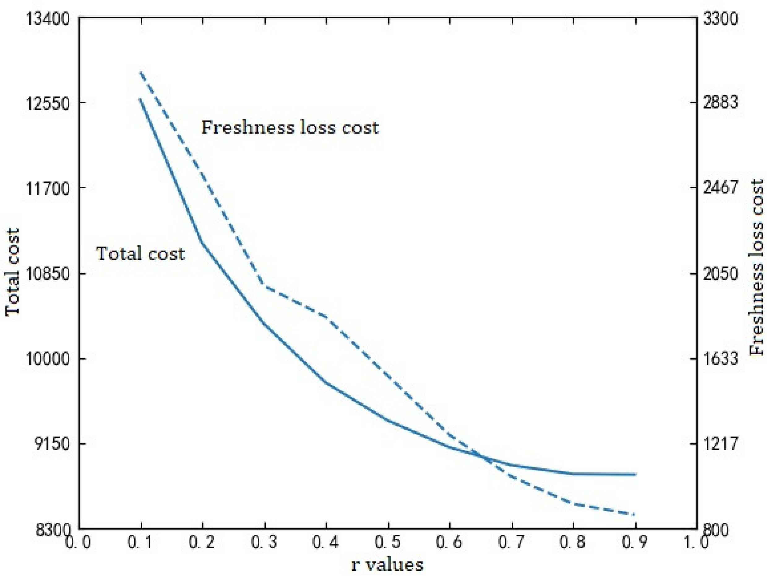
• Experimental results of different regulatory factors show that the difference in time sensitivity of fresh agricultural products has a great impact on the total cost and distribution plan. With the reduction of time sensitivity of fresh agricultural products, the total cost will be greatly reduced, and the proportion of fresh loss cost to total cost will also be greatly reduced.
• The experiments on the relationship between itemized costs show that carbon emission costs account for the lowest proportion of total costs. Assign weight to each itemized cost. If the weight of carbon emission cost increases, the cost of carbon emission will decrease while the total cost will increase. If the weight of distribution cost and freshness loss cost increases, the total cost decreases. That is, when companies focus on reducing carbon emissions, the total cost increases.
• In this paper, standard calculation examples were used for the experiment. The standard calculation examples lack road slope data, which have an impact on the carbon emissions of vehicles. Future studies can be conducted on the basis of real cases with road slope, and more accurate conclusions on carbon emissions will be drawn.

6. Conclusions

In order to reduce carbon emissions and reduce the total cost of fresh product distribution, this paper constructed the TDGVRPSTW model and designed the variable neighborhood adaptive genetic algorithm to solve the problem. The experimental results which were constructed based on the standard example show that the proposed approach has a faster convergence speed and better optimization ability than the comparison method. Through experiments, this paper found that the geographical distribution of customers will affect the proportion of each part in the total cost. The experiment also explores the influence of the time-sensitive adjustment factor in the freshness loss coefficient function on delivery planning. The last experiment explored the relationship between different costs in the total cost.

Based on the experimental findings in this paper, the following recommendations are put forward.

• In practice, the enterprise should rationally choose the optimization goal and arrange the vehicle distribution plan according to the distribution law of customers, the time-sensitivity of fresh products, the customer time window, and the time-varying road network conditions.
• Before making a distribution plan, enterprises should have a reasonable estimate of the time sensitivity of fresh agricultural products to be distributed. When agricultural products are time-sensitive, freshness loss has a great impact on the total cost, and enterprises should pay attention to reducing freshness loss. When agricultural products are time-insensitive, freshness loss has little impact on the total cost, and enterprises can give priority to other cost indicators, such as carbon emissions.
• The proportion of carbon emission cost in the total cost is relatively low, so the carbon trading price can be appropriately raised to attract enterprises to pay attention to the reducing of carbon emission.
• The preference of enterprises for different optimization objectives in the total cost will significantly affect the total cost, so the weight should be allocated according to the actual situation to achieve the purpose of enterprises.

This paper is only an exploratory study on the time-dependent green vehicle routing problem with soft time window constraints. The following cases are worthy of further study.

• The research in this paper is based on the same fresh agricultural products transported by all vehicles, but in reality, the fresh agricultural products transported by each vehicle may be different, and a variety of fresh agricultural products may be mixed in one vehicle. In these cases, the relationship between freshness loss and total cost, as well as the influence of time sensitivity of agricultural products on distribution plan, need to be further explored.
• Furthermore, consider the situation of customer orders. A customer’s order may contain a variety of fresh agricultural products, and the splitting and merging of customer orders will make transportation more efficient and should be considered, as well as how to do the splitting and merging of orders. These problems require further study.
• The study in this paper is based on a static scenario, and a study of the dynamic scenario of TDGVRPSTW has not been carried out. The design of research methods in dynamic situations can become the direction of future research.

References

1. Lin, C.; Choy, K.; Ho, G.; Chung, S.; Lam, H. Survey of Green Vehicle Routing Problem: Past and future trends. Expert Syst. Appl. 2014, 41, 1118–1138. [Google Scholar] [CrossRef]
2. Bektaş, T.; Laporte, G. The Pollution-Routing Problem. Transp. Res. Part B Methodol. 2011, 45, 1232–1250. [Google Scholar] [CrossRef]
3. Erdoğan, S.; Miller-Hooks, E. A Green Vehicle Routing Problem. Transp. Res. Part E Logist. Transp. Rev. 2012, 48, 100–114. [Google Scholar] [CrossRef]
4. Chang, D.J.; Morlok, E.K. Vehicle Speed Profiles to Minimize Work and Fuel Consumption. J. Transp. Eng. 2005, 131, 173–182. [Google Scholar] [CrossRef]
5. Suzuki, Y. A dual-objective metaheuristic approach to solve practical pollution routing problem. Int. J. Prod. Econ. 2016, 176, 143–153. [Google Scholar] [CrossRef]
6. Li, J.; Wang, R.; Li, T.; Lu, Z.; Pardalos, P.M. Benefit analysis of shared depot resources for multi-depot vehicle routing problem with fuel consumption. Transp. Res. Part D Transp. Environ. 2018, 59, 417–432. [Google Scholar] [CrossRef]
7. Alinaghian, M.; Naderipour, M. A novel comprehensive macroscopic model for time-dependent vehicle routing problem with multi-alternative graph to reduce fuel consumption: A case study. Comput. Ind. Eng. 2016, 99, 210–222. [Google Scholar] [CrossRef]
8. Manerba, D.; Mansini, R.; Zanotti, R. Attended Home Delivery: Reducing last-mile environmental impact by changing customer habits. IFAC-PapersOnLine 2018, 51, 55–60. [Google Scholar] [CrossRef]
9. Yu, Y.; Wang, S.; Wang, J.; Huang, M. A branch-and-price algorithm for the heterogeneous fleet green vehicle routing problem with time windows. Transp. Res. Part B Methodol. 2019, 122, 511–527. [Google Scholar] [CrossRef]
10. Ehmke, J.F.; Campbell, A.; Thomas, B.W. Vehicle routing to minimize time-dependent emissions in urban areas. Eur. J. Oper. Res. 2016, 251, 478–494. [Google Scholar] [CrossRef]
11. Micale, R.; Marannano, G.; Giallanza, A.; Miglietta, P.; Agnusdei, G.; La Scalia, G. Sustainable vehicle routing based on firefly algorithm and TOPSIS methodology. Sustain. Future 2019, 1, 100001. [Google Scholar] [CrossRef]
12. Fukasawa, R.; He, Q.; Song, Y. A disjunctive convex programming approach to the pollution-routing problem. Transp. Res. Part B Methodol. 2016, 94, 61–79. [Google Scholar] [CrossRef]
13. Soysal, M.; Çimen, M.; Demir, E. On the mathematical modeling of green one-to-one pickup and delivery problem with road segmentation. J. Clean. Prod. 2018, 174, 1664–1678. [Google Scholar] [CrossRef] [Green Version]
14. Giallanza, A.; Puma, G.L. Fuzzy green vehicle routing problem for designing a three echelons supply chain. J. Clean. Prod. 2020, 259, 120774. [Google Scholar] [CrossRef]
15. Zulvia, F.E.; Kuo, R.; Nugroho, D.Y. A many-objective gradient evolution algorithm for solving a green vehicle routing problem with time windows and time dependency for perishable products. J. Clean. Prod. 2020, 242, 118428. [Google Scholar] [CrossRef]
16. Bravo, M.; Rojas, L.P.; Parada, V. An evolutionary algorithm for the multi-objective pick-up and delivery pollution-routing problem. Int. Trans. Oper. Res. 2017, 26, 302–317. [Google Scholar] [CrossRef]
17. Wu, D.; Liu, Y.; Zhou, K.; Li, K.; Li, J. A multi-objective particle swarm optimization algorithm based on human social behavior for environmental economics dispatch problems. Environ. Eng. Manag. J. 2019, 18, 1599–1607. [Google Scholar] [CrossRef]
18. Wu, D.Q.; Dong, M.; Li, H.Y. Vehicle Routing Problem with Time Windows Using Multi-Objective Co-Evolutionary Approach. Int. J. Simul. Model. 2016, 15, 742–753. [Google Scholar] [CrossRef]
19. Wu, D.; Huo, J.; Zhang, G.; Zhang, W. Minimization of Logistics Cost and Carbon Emissions Based on Quantum Particle Swarm Optimization. Sustainability 2018, 10, 3791. [Google Scholar] [CrossRef] [Green Version]
20. Muñoz-Villamizar, A.; Velázquez-Martínez, J.C.; Mejía-Argueta, C.; Gámez-Pérez, K. The impact of shipment consolidation strategies for green home delivery: A case study in a Mexican retail company. Int. J. Prod. Res. 2021, 1–18. [Google Scholar] [CrossRef]
21. Liu, C.; Kou, G.; Zhou, X.; Peng, Y.; Sheng, H.; Alsaadi, F.E. Time-dependent vehicle routing problem with time windows of city logistics with a congestion avoidance approach. Knowl.-Based Syst. 2020, 188, 104813. [Google Scholar] [CrossRef]
22. Xiao, Y.; Konak, A. The heterogeneous green vehicle routing and scheduling problem with time-varying traffic congestion. Transp. Res. Part E Logist. Transp. Rev. 2016, 88, 146–166. [Google Scholar] [CrossRef]
23. Li, H.; Zhang, L.; Lv, T.; Chang, X. The two-echelon time-constrained vehicle routing problem in linehaul-delivery systems. Transp. Res. Part B Methodol. 2016, 94, 231–245. [Google Scholar] [CrossRef]
24. Wang, Y.; Assogba, K.; Fan, J.; Xu, M.; Liu, Y.; Wang, H. Multi-depot green vehicle routing problem with shared transportation resource: Integration of time-dependent speed and piecewise penalty cost. J. Clean. Prod. 2019, 232, 12–29. [Google Scholar] [CrossRef]
25. Franceschetti, A.; Demir, E.; Honhon, D.; Van Woensel, T.; Laporte, G.; Stobbe, M. A metaheuristic for the time-dependent pollution-routing problem. Eur. J. Oper. Res. 2017, 259, 972–991. [Google Scholar] [CrossRef] [Green Version]
26. Sadati, M.E.H.; Çatay, B. A hybrid variable neighborhood search approach for the multi-depot green vehicle routing problem. Transp. Res. Part E Logist. Transp. Rev. 2021, 149, 102293. [Google Scholar] [CrossRef]
27. Deng, W.; Xu, J.; Zhao, H.; Song, Y. A Novel Gate Resource Allocation Method Using Improved PSO-Based QEA. IEEE Trans. Intell. Transp. Syst. 2020, 1–9. [Google Scholar] [CrossRef]
28. Deng, W.; Xu, J.; Gao, X.-Z.; Zhao, H. An Enhanced MSIQDE Algorithm With Novel Multiple Strategies for Global Optimization Problems. IEEE Trans. Syst. Man Cybern. Syst. 2020, 1–10. [Google Scholar] [CrossRef]
29. Deng, W.; Shang, S.; Cai, X.; Zhao, H.; Zhou, Y.; Chen, H.; Deng, W. Quantum differential evolution with cooperative coevolution framework and hybrid mutation strategy for large scale optimization. Knowl.-Based Syst. 2021, 224, 107080. [Google Scholar] [CrossRef]
30. Rahbari, A.; Nasiri, M.M.; Werner, F.; Musavi, M.; Jolai, F. The vehicle routing and scheduling problem with cross-docking for perishable products under uncertainty: Two robust bi-objective models. Appl. Math. Model. 2019, 70, 605–625. [Google Scholar] [CrossRef]
31. Alkaabneh, F.; Diabat, A.; Gao, H.O. Benders decomposition for the inventory vehicle routing problem with perishable products and environmental costs. Comput. Oper. Res. 2020, 113, 104751. [Google Scholar] [CrossRef]
32. Shao, J.; Cao, Q.; Shen, M.; Sun, Y. Research on Multi-objective Optimization for Fresh products VRP Problem. Ind. Eng. Manag. Syst. 2015, 20, 122–127+134. [Google Scholar]
33. Zhou, X.C.; Zhou, K.J.; Wang, L.; Liu, C.S.; Huang, X.B. Review of green vehicle routing model and its algorithm in logistics distribution. Syst. Eng. Theory Pract. 2021, 41, 213–230. [Google Scholar]
34. Fu, Z.; Eglese, R.W.; Li, L. A unified tabu search algorithm for vehicle routing problems with soft time windows. J. Oper. Res. Soc. 2008, 59, 663–673. [Google Scholar] [CrossRef] [Green Version]
35. Han, Y.J.; Peng, Y.F.; Wei, H.; Shi, B.L. Hyper-heuristic genetic algorithm for vehicle routing problem with soft time windows. Comput. Integr. Manuf. Syst. 2019, 25, 2571–2579. [Google Scholar]
36. Pamosoaji, A.K.; Dewa, P.K.; Krisnanta, J.V. Proposed Modified Clarke-Wright Saving Algorithm for Capacitated Vehicle Routing Problem. J. Ind. Eng. Manag. 2019, 1, 9–15. [Google Scholar] [CrossRef]
37. Solomon, M.M. Algorithms for the Vehicle Routing and Scheduling Problems with Time Window Constraints. Oper. Res. 1987, 35, 254–265. [Google Scholar] [CrossRef] [Green Version]
38. Vidal, T.; Crainic, T.G.; Gendreau, M.; Prins, C. Heuristics for multi-attribute vehicle routing problems: A survey and synthesis. Eur. J. Oper. Res. 2013, 231, 1–21. [Google Scholar] [CrossRef]
39. Liu, Z.; Chen, Y.; Li, J.; Zhang, D. Spatiotemporal-Dependent Vehicle Routing Problem Considering Carbon Emissions. Discret. Dyn. Nat. Soc. 2021, 2021, 9729784. [Google Scholar] [CrossRef]
40. Ghannadpour, S.F.; Zarrabi, A. Multi-objective heterogeneous vehicle routing and scheduling problem with energy minimizing. Swarm Evol. Comput. 2019, 44, 728–747. [Google Scholar] [CrossRef]
Figure 2. Penalty cost curve under the broken line soft time window.
Applsci 11 10579 g002
Figure 3. Algorithm flow chart.
Applsci 11 10579 g003
Figure 4. Flowchart of the saving algorithm and nearest neighbor insertion algorithm. (a) The flowchart of improved CW saving algorithm; (b) the flowchart of nearest neighbor insertion algorithm.
Applsci 11 10579 g004
Figure 5. Crossover mutation diagram. (a) An example of a crossover process; (b) an example of a mutation process.
Applsci 11 10579 g005
Figure 6. Variable neighborhood descent operator. (a) An example of gene fragment inversion process; (b) an example of single locus insertion process; (c) an example of double locus insertion process.
Applsci 11 10579 g006
Figure 7. Optimal distribution roadmap in the comparison experiment.
Applsci 11 10579 g007
Figure 8. Adjustment factor and cost curve.
Applsci 11 10579 g008