Abstract
In this work, we present a numerical study on the development length (the length from the channel inlet required for the velocity to reach of its fully-developed value) of a pressure-driven viscoelastic fluid flow (between parallel plates) modelled by the generalised Phan–Thien and Tanner (gPTT) constitutive equation. The governing equations are solved using the finite-difference method, and, a thorough analysis on the effect of the model parameters and is presented. The numerical results showed that in the creeping flow limit (), the development length for the velocity exhibits a non-monotonic behaviour. The development length increases with . For low values of , the highest value of the development length is obtained for ; for high values of , the highest value of the development length is obtained for . This work also considers the influence of the elasticity number.
1. Introduction
A variety of functional applications are based on the premise that the flow is fully developed. It is assumed that after a certain time the fluid has travelled a certain length (development length—L) along the channel, after which the flow no longer changes in the direction of flow. This is used, for example, in extrusion dies, lab-on-a-ship, etc. [1,2,3].
The development length of Newtonian flows in channels and pipes (see Figure 1) is well understood [4].
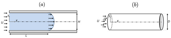
Figure 1.
Schematic of the channel and pipe geometries used for the study of the development length. (a) Channel flow. (b) Pipe flow.
Durst et al. [4] developed two correlations between L (the distance the fluid travels to become fully developed) and the Reynolds number, , where U is the imposed mean inlet velocity, is the fluid density, H is the width of the channel (for pipes, one should replace H by D-diameter), and is the Newtonian viscosity. These correlations are given by,
and predict well the development length for channel and pipe flows, respectively. For other works on the development length of Newtonian fluids please consult the following references [5,6,7,8,9,10].
For generalised Newtonian fluids (with varying viscosity), several works have been proposed in the literature [11,12,13,14,15,16,17,18,19]. We would like to highlight the works of Fernandes et al. [19] and Poole and Ridley [18], in which they presented two correlations for the development length in channel and pipe flows of power-law fluids (the viscosity is a function of the second invariant of the deformation tensor, (for simple flows, is simply the shear rate). The viscosity is then given by ). The correlations are given by,
for channel and pipe flows, respectively. Here, , , and . Note the increasing complexity in the correlations when going from a Newtonian to a power-law fluid.
In the case of viscoelastic fluids, the number of papers on this topic is smaller. This is due to the complexity of viscoelastic flows, such as the presence of singularities at the entrance of the channel, overshoots in the velocity profile, and the high Weissenberg number problem.
We would like to highlight the work of Na and Yoo [20] in which they perform numerical simulations to determine the development length of an Oldroyd-B fluid and conclude that the development length (for a fixed ) increases slightly with the Weissenberg number, (where is the relaxation time of the fluid in seconds), but is more strongly affected by . Liang [1] proposed a theoretical work for the development length of viscoelastic fluids entering an extrusion die. They presented an expression for estimating the length of the entrance region, which has applications in the extrusion industry. In the work by Philippou et al. [10] the authors present a study on the flow development of a Bingham plastic fluid in tubes and channels considering the Papanastasiou regularisation and the finite element method. They considered the Navier’s slip law at the wall and concluded that as slip increases, the development length initially increases exhibiting a global maximum before vanishing rapidly above the critical point corresponding to sliding flow. More recently, Yapici et al. [21] presented a study on the development length of steady flows of Oldroyd-B and Phan–Thien–Tanner (PTT) fluids through a two-dimensional rectangular channel and concluded that the development length determined for the Oldroyd-B fluid varies exponentially with and linearly for the linear PTT model; they also concluded that higher entry lengths are predicted with increasing (at fixed ).
To remove the unstable numerical effect of the singularity at the entrance corner, a continuous inlet velocity profile is used in both works of Na et al. [20] and Yapici et al. [21]. This regularised profile can affect the true development length, so in the work of Guilherme [22] the log-conformation formulation [23,24,25] is used, which reduces the rate of increase of the stresses and thus avoids the need to introduce artificial inlet velocity profiles.
It should be noted that the development of a correlation for the prediction of the development length of such complex fluids is still difficult due to the high number of parameters involved and the fact that it is model dependent.
Here we follow the work of Guilherme [22], where a detailed analysis of the development length of the linear PTT model is performed. We extend his work to the exponential and generalised PTT models [22,26,27].
This work is organised as follows. First, we present the differential equations to be solved and their numerical solution. In Section 3, we present the geometry and the meshes. In Section 4, we perform a validation of the numerical method and the meshes, using Newtonian benchmark results. In Section 5, we present and discuss the results for viscoelastic fluids. The paper ends with the main conclusions in Section 6.
2. Governing Equations
The equations governing the flow of an incompressible fluid, under isothermal conditions, are the continuity,
and the momentum equations,
where is the velocity vector, p is the pressure, is the stress tensor (to be defined later), is the mass density, and represents the external forces. Note that all variables are dimensionless, with: , , , , (the ∗ represents the dimensional variable).
In order to achieve a closed system of equations, a constitutive equation for the extra-stress tensor, , is required. Recently, Ferrás et al. [27] proposed a new differential model based on the Phan–Thien–Tanner constitutive equation [26] (see also [28]). This new model considers a more general function for the rate of destruction of junctions, the Mittag–Leffler function, where one or two fitting parameters are included, in order to achieve additional fitting flexibility.
The Mittag–Leffler function is defined as,
with , being real and positive. is the gamma function, given by:
when , the Mittag–Leffler function reduces to the exponential function, and when the original one-parameter Mittag–Leffler function, is obtained.
The constitutive equation is given by:
where is the trace of the stress tensor, is the Weissenberg number, is the Reynolds number ( is the kinematic viscosity), is the rate of deformation tensor, is the elastic stress, and is the viscosity coefficient, where is the total shear viscosity ( is the solvent/Newtonian viscosity, is the polymer viscosity) and represents the Gordon–Schowalter derivative.
The stress function, , is given by a new formulation that imparts more flexibility and accuracy to the model predictions, as discussed in [27,29,30]. It is given by:
where represents the extensibility parameter, is the Gamma function, and the normalisation is used to ensure that , for all choices of .
3. Numerical Method
The numerical method used in this work is based on finite differences. It can deal with tree-like mesh grids (see Figure 2b) and allows fast Cartesian discretizations, flexibility and accuracy, and local mesh refinement. In order to fit the discretization stencil near the interfaces between grid elements of different sizes, a robust method based on a moving least squares meshless interpolation technique is used to compute the weights of the finite difference approximation in a given hierarchical grid, allowing complex mesh configurations and preserving the overall accuracy of the resulting method.
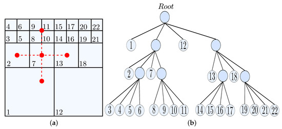
Figure 2.
(a) Mesh refinement and the need to use an adaptive least squares method; (b) dependency tree.
Figure 2a shows a schematic representation of the mesh refinement. Note that some of the points (variables) of the computational cells (red dots) must be approximated because they are not located in the center of the cell (e.g., the center of computational cell 1 is not the same as the location of the red dot used to compute the derivative of the property being evaluated). To solve this problem, we use a special adaptive least square interpolation (). The method is known as HiG-Flow, and a detailed mathematical explanation can be found in [31,32].
For the numerical solution of the Navier–Stokes equations together with the constitutive equation given by the gPTT model, the momentum Equation (6) is rewritten:
From Equation (9), the rheological constitutive equation can be written as:
where is given by Equation (14),
and the parameter accounts for the slip between the molecular network and the continuous medium. For there is no slip and the motion becomes affine. The parameter leads to a non-zero second normal-stress difference in shear, resulting in secondary flows in ducts having non-circular cross-sections. Since in this work we only consider 2D flows, and, due to the high number of parameters involved in the numerical simulations and the gPTT model itself, we have only considered the case when .
3.1. Calculation of and
To calculate the velocity and pressure fields, we use the incremental projection method by Chorin [33], that uncouples the mass conservation and momentum equations, given by Equations (5) and (6), respectively. This method allows one to obtain an intermediate velocity field from Equation (11). In the HiG-Flow methodology, this Equation (11) can be approximated using an explicit Euler method, Runge–Kutta RK-2 or RK-4, or, the semi-implicit Euler methods, Cranck–Nicolson, and BDF2. One can also choose a spatial discretization orders of 2 or 4. One can use the the convective central schemes or Upwind (order 1), or, schemes of order 2 like the Cubista [34] and Quick [35].
In this work an Implicit Euler scheme together with a second order spatial approximation and an Upwind Cubista scheme for the convective terms, is used:
here, is the time step, n represents the known values of velocity, stress, and pressure at instant n, and represents the new velocity field values (unknown) to be obtained from the solution of the equation. At the inlet, (see Figure 3) we consider a constant velocity profile, (the stress components are set to 0) and at the outlet, we assume fully developed boundary conditions (Neumann boundary conditions) for the velocity and stress (the pressure is imposed). Finally, at the walls ( and ), we have the empirical no-slip boundary condition ().
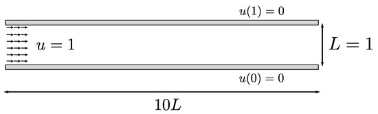
Figure 3.
Dimensionless representation of the channel domain.
Using the projection method, it is well known that the velocity field obtained from Equation (15) may not satisfy the mass conservation equation. Therefore, in order to solve this problem, the equation for the potential is solved,
and the Helmholtz–Hodge decomposition (see [31,32,36] for more details) is used to correct the previous non-conservative velocity field ,
The new velocity field satisfies the mass conservation equation. Finally, the pressure is updated .
3.2. Calculation of the Extra-Stress Tensor
The velocity and pressure fields were obtained in the previous subsection. We now aim to obtain the extra-stress tensor field. Equation (13) is solved using the Explicit Euler method, and, to calculate (see Equation (14)), the Mittag–Leffler function and the term are obtained numerically from Equation (18) and the approximations presented in the work by R. Gorenflo, J. Loutchko, and Y. Luchko [37],
The numerical implementation of the Mittag–Leffler function follows the work by Davide Verotta and Eduardo Mendes [38] (developed in Fortran), which is adapted in this work to C++. The original fortran code is based on a Matlab function developed by Igor Podlubny and Martin Kacena [39] which, in turn, was based on the reference [37].
4. Geometry and Meshes
4.1. Geometry
Due to the low values considered in this work, and based on the few literature results on the development length of viscoelastic fluids, we considered a geometry where the length of the channel is fixed at 10 times its width (Figure 3).
4.2. Meshes
We performed simulations considering more than 8 levels of mesh refinement. After some numerical experiments, the following meshes were considered:
- —uniform mesh with 160 × 16 computational cells and a minimum and mesh spacing of 0.0625;
- —uniform mesh with 320 × 32 computational cells and a minimum and mesh spacing of 0.03125;
- —uniform mesh with 640 × 64 computational cells and a minimum and mesh spacing of 0.015625.
The tree meshes are shown in Figure 4.
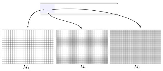
Figure 4.
Three consequently refined uniform meshes used in this work.
Numerical simulations were also performed considering a mesh with additional refinement in the centerline of the channel, as shown in Figure 5. A total number of 16,000 cells was used.
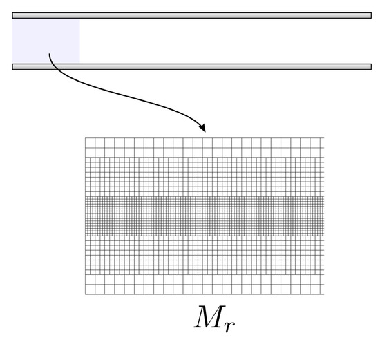
Figure 5.
Mesh with refinement in the centerline region.
5. Validation of the Numerical Method
The validation of the numerical method is performed in two steps. First, the numerically-determined fully-developed velocities and stresses are compared with the analytical solution [27]. Then, the development length obtained for the gPTT model with (almost Newtonian fluid) is compared with the benchmark results of Durst et al. [4].
5.1. Comparison with the Analytical Solution
Figure 6 shows a comparison between the analytical solution (solid line) and the numerical solution (symbols) for mesh with , and ( was set to 0). In Figure 6a we have and and in Figure 6b and .
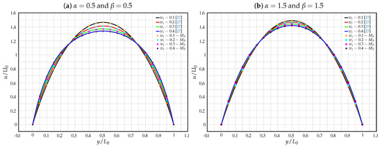
Figure 6.
Comparison between the analytical solution (solid line) and the numerical solution (symbols) for mesh with , , and ( was set to 0). (a) and . (b) and .
It can be seen that an excellent agreement is obtained between the analytical and numerical solutions for all the considered values of , which underlines the robustness of the numerical method and the meshes.
For lower values of and , we obtain a higher destruction rate of the junctions in the gPTT model. Note that the typical viscoelastic velocity profile is more flattened for lower values of and . In this case, the different values of have a stronger impact on the model’s behaviour. This result is similar to those found in the literature comparing linear and exponential functions of the trace of the stress tensor.
5.2. Comparison with the Development Length of a Newtonian Fluid
In the limiting case of we obtain a Newtonian fluid. Therefore, we considered and performed simulations for the development length of a gPTT fluid, using the geometry shown in Figure 4. We considered a Reynolds number in the range , where the nonlinear variation of the development length with is more pronounced. The other parameters of the model were set as follows: , , , .
Figure 7a shows a comparison between the development length obtained with the gPTT model, a Newtonian fluid, and that obtained by the Durst et al. [4] correlation for the variation of the development length with (see Equation (1)). The three results practically overlap, proving once again the robustness of the numerical method.
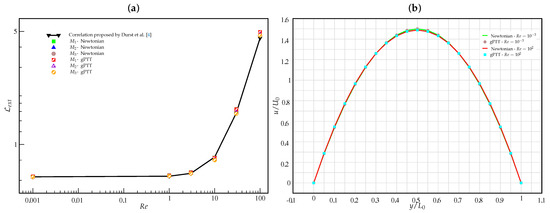
Figure 7.
(a) Comparison between the development length obtained with the gPTT model (with ), a Newtonian fluid, and the correlation proposed by Durst et al. [4], for three different meshes , , and . (b) Velocity profiles in the fully developed region for mesh , considering the gPTT and Newtonian models, for and .
As increases, the results for the gPTT model in the coarse mesh are slightly higher than those obtained for the Newtonian fluid and the correlation. However, in the nonlinear domain the results are quite accurate.
Figure 7b shows the velocity profiles obtained in the fully developed region of the channel (mesh ) considering the gPTT and Newtonian models for and .
Again, there is excellent agreement between the two solutions for the two different values of . This shows that the value of is a good approximation for the Newtonian fluid.
Based on these results, the numerical code is now able to predict the development length of the fluid modelled by the gPTT model considering a wider range of numbers.
6. Development Length of a gPTT Fluid
6.1. Simulations
We performed a large number of simulations by considering = 0.1, 0.2, 0.3, 0.4, 0.5, 0.6, 0.7, 0.8, 0.9, 1, creeping flow (), and the following combination of and parameters:
- -Meshes , , , -
- -Meshes , , , -
- -Meshes , , , -
- -Meshes , , , -
- -Meshes , -
- -Meshes , -
- -Meshes , -
- -Meshes , -
- -Meshes , -
- -Meshes , -
This gives a total number of 132 simulations. The simulations with the finest mesh took about 15 h each.
The first set of 72 simulations allowed conclusions to be drawn about the convergence of the numerical method and the error in calculating the development length using the Richardson extrapolation technique. Based on the results of these simulations, a second set of simulations was performed for higher values of using meshes (see Figure 4) and (see Figure 5). These meshes were chosen based on a trade-off between accuracy and computational time.
6.2. Creeping Flow
6.2.1. Case of
The development length, determined as the length from the channel inlet required for the velocity to reach of its fully developed value, and denoted here as , is shown in Table 1. The results are shown only for up to 0.4, since convergence problems for finer meshes are observed for higher values of . The main problem arises from the singularity at the entrance corner of the channel, which generates an error that propagates along the channel (for more details, see [24,25]).

Table 1.
Benchmark development length values for the velocity ().
Note that the error is higher at the lowest and highest values of and , being more pronounced when and are low. The maximum error was and was obtained, as expected, for and . It should be noted that the errors are quite low and therefore these solutions can be used as benchmarks.
Figure 8 shows the development lengths for mesh presented in Table 1. A nonlinear variation of the development length with , , and is observed.
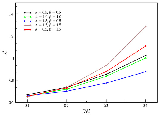
Figure 8.
Development length as a function of considering () and mesh .
The development length increases with , with viscoelastic effects delaying the diffusion and convection of information from the walls to the center of the channel. This diffusion and convection is also strongly influenced by the parameters of the Mittag–Leffler function. For low values of , the highest value of the development length is obtained for ; for high values of , the highest value of the development length is obtained for . A molecular continuum explanation of this phenomenon is not an easy task. At high and values, the rate of destruction of the junctions is lower than at low and values. This means that when values are low and the rate of junction destruction is high, information travels slowly from the wall to the center of the channel (compared to when the rate of junction destruction is low). The opposite was expected. Note that in this case the development lengths are very similar for all tested values of and , and therefore the influence of these parameters on the development length is small. These results can be justified by the low value of .
As increases, the highest value of development length is reached with a low rate of destruction of junctions. This result can be justified by the fact that as the rate of destruction of the junctions decreases, the information is transmitted more slowly due to the small number of new contacts between the strands representing the molecules.
6.2.2. Case of
In addition to the error arising at the entrance corner due to a singularity, we also have the problem of the development length, which takes into account of the fully developed maximum velocity and may not work so well in an intermediate mesh as , for higher . This leads to an increased difficulty for the numerical method to capture for the mesh .
Therefore, to capture the essence of the development length for higher values, we considered another development length, (length from channel entry required for the velocity to reach of its fully-developed value), which is less restrictive.
The results obtained for are shown in Figure 9 for mesh and Table 2 for the three meshes (along with the extrapolated development length value).
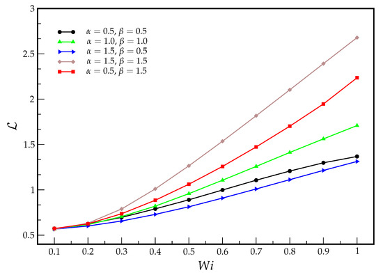
Figure 9.
Development length as a function of considering () and mesh .
Table 2.
Benchmark development length values for the velocity ().
The results obtained follow the same trend observed in the case , with some minor differences. The development length is initially higher for the case than for the case , until , where the growth rate of becomes larger with for . For , the two development lengths are quite similar.
For , we obtain a development length of for and a development length of for (and for ). Again, these results are consistent with the idea that the higher the rate of destruction of junctions, the smaller the development length (information travels faster across the channel).
Figure 10, Figure 11 and Figure 12 show the different velocity profiles obtained at 10 different sections of the channel. The first numerical velocity profile is taken at () and the last profile is taken at the middle of the channel ( or ).
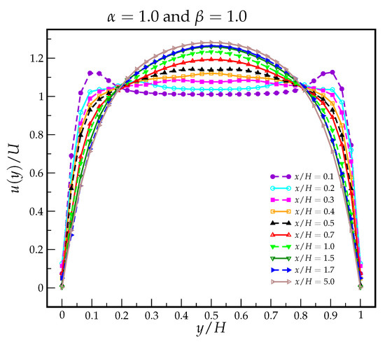
Figure 10.
Velocity profiles obtained at 10 different sections of the channel for , , .
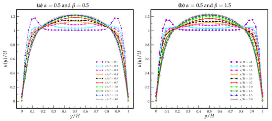
Figure 11.
Velocity profiles obtained at 10 different sections of the channel for . (a) , ; (b) , .
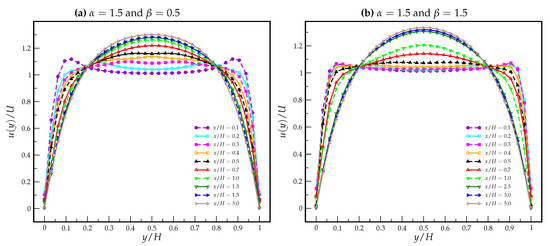
Figure 12.
Velocity profiles obtained at 10 different sections of the channel for . (a) , ; (b) , .
Figure 10 shows the reference velocity profiles obtained for the classical case of an exponential PTT model (). The velocity profile evolves from a plug profile in the center of the channel (for profiles near the inlet) to the typical parabolic profile (in the fully developed region). Note the overshoots near the walls that occur when the fluid is still developing. This is due to the different characteristic times of the fluid and the diffusion of information moving from the walls ( and ) to the center of the channel ().
Figure 11 shows the velocity profiles obtained for and . It can be seen that the overshoots are stronger near the inlet (compared to the exponential PTT model) and that a lower maximum velocity is obtained when the fluid is fully developed. The influence of the parameter is residual.
Figure 12 shows the velocity profiles obtained for and , . In Figure 12a it can be seen that the overshoots near the inlet resemble the case of the exponential PTT model, and that the maximum velocity increases again. The main difference is that the plug profile is now less pronounced. When increases (Figure 12b), one can observe a dramatic change in the evolution of the velocity profiles. The velocity overshoots are almost suppressed and the maximum velocity increases. This means that the rate of destruction of junctions improves the diffusion of information.
6.3. The Influence of the Elasticity Number
In this subsection we study the influence of the elasticity number, , on the development length of the gPTT model. We consider three different values for (), , and two different values for , and . The mesh used for the simulation is .
Table 3.
Influence of the Elasticity number, , on the development length of the gPTT model. , , and for , .
Table 4.
Influence of the Elasticity number, , on the development length of the gPTT model. , , and for , .
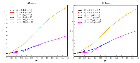
Figure 13.
Influence of the elasticity number, , on the development length of the gPTT model. We consider three different values of (), and two different values of , and .
As expected, the results for low values of are consistent with those obtained earlier in this work (see previous sections for more details). The results obtained for the different definitions of the development length are qualitatively similar. However, higher values of development length are obtained for , as expected.
For high values of (), the influence of the elasticity number seems to be neglected by the fluid, since we obtain the same development length for and . For the results are quite different, which is due to the low values of compared to the and cases.
For , the rate of destruction of junctions increases and the development length decreases by about half. Again, the and cases show similar development lengths, which is due to the similar values of and the almost creeping flow conditions.
The results show that for the tested ranges of , , and , no critical value is found for . This is due to the fact that Mach’s Elastic number is less than 1.
7. Conclusions
In this work, we present a numerical study on the development length of a pressure-driven viscoelastic fluid flow (between parallel plates) modelled by the generalised Phan–Thien and Tanner (gPTT) constitutive equation. The governing equations are solved using the finite-difference method, and, a thorough analysis on the effect of the model parameters and is presented. We consider two different definition of the development length: The length from the channel inlet required for the velocity to reach (and ) of its fully-developed value.
The numerical results showed that the in the creeping flow limit (i.e., ), the development length for the velocity exhibits a non-monotonic behaviour. The development length increases with , with viscoelastic effects delaying the diffusion and convection of information from the walls to the center of the channel. For low values of , the highest value of the development length is obtained for ; for high values of , the highest value of the development length is obtained for . At high and values, the rate of destruction of the junctions is lower than at low and values. This means that when values are low and the rate of junction destruction is high, information travels slowly from the wall to the center of the channel (compared to when the rate of junction destruction is low). The opposite was expected. Note that in this case, the development lengths are very similar for all tested values of and , and therefore the influence of these parameters on the development length is small. These results can be justified by the low value of .
As increases, the highest value of development length is reached with a low rate of destruction of junctions. This result can be justified by the fact that as the rate of destruction of the junctions decreases, the information is transmitted more slowly due to the small number of new contacts between the strands representing the molecules.
We also studied the influence of the elasticity number, , on the development length of the gPTT model. As expected, the results for low values of are consistent with those obtained for creeping flow. For high values of (), the influence of the elasticity number seems to be neglected by the fluid, since we obtain the same development length for and . For , the results are quite different, which is due to the low values of compared to the and cases. For , the rate of destruction of junctions increases and the development length decreases by about half. Again, the and cases show similar development lengths, which is due to the similar values of and the almost creeping flow conditions.
Author Contributions
Conceptualization, J.B., L.L.F., A.M.A., R.T.L. and A.C.; methodology, J.B., L.L.F., A.M.A., R.T.L. and A.C.; software, J.B., R.T.L. and A.C.; validation, J.B., L.L.F., A.M.A., R.T.L. and A.C.; formal analysis, J.B., L.L.F., A.M.A., R.T.L. and A.C.; investigation, J.B., L.L.F., A.M.A., R.T.L. and A.C.; writing—original draft preparation, J.B., L.L.F., A.M.A., R.T.L. and A.C.; writing—review and editing, J.B., L.L.F., A.M.A., R.T.L. and A.C.; funding acquisition, J.B., L.L.F., A.M.A., R.T.L. and A.C. All authors have read and agreed to the published version of the manuscript.
Funding
This research was funded by FCT—Fundação para a Ciência e a Tecnologia, through projects UIDB/00532/2020 and UIDP/00532/2020 of CEFT (Centro de Estudos de Fenómenos de Transporte), and through PTDC/EMS-ENE/3362/2014 and POCI-01-0145-FEDER-016665—funded by FEDER funds through COMPETE2020—Programa Operacional Competitividade e Internacionalização (POCI) and by national funds through FCT. It was also funded by FCT through the CMAT projects UIDB/00013/2020 and UIDP/00013/2020 (CMAT—Centro de Matemática e Aplicações); and was funded by Fapesp-Fundação de Amparo à Pesquisa do Estado de São Paulo, Fapesp-2017/21105-6 and Petrobrás (Project 0050.0075367.12.9). Research was carried out using the computational resources of the Center for Mathematical Sciences Applied to Industry (CeMEAI), funded by FAPESP grant 2013/07375-0.
Institutional Review Board Statement
Not applicable.
Informed Consent Statement
Not applicable.
Data Availability Statement
Not applicable.
Acknowledgments
J. Bertoco acknowledges the support by Faculdade de Ciências Exatas e Tecnológicas—FACET—UNEMAT—MT. J. Bertoco, R.T. Leiva, and A. Castelo acknowledge the support by ICMC—Instituto de Ciências Matemáticas e de Computação, Departamento de Matemática e Estatística, USP, São Carlos, SP. A.M. Afonso acknowledges the support by CEFT (Centro de Estudos de Fenómenos de Transporte). L.L. Ferrás acknowledges the support by CMAT—Centre of Mathematics from the University of Minho.
Conflicts of Interest
The authors declare no conflict of interest.
Abbreviations
The following abbreviations are used in this manuscript:
| PTT | Phan–Thien and Tanner |
| gPTT | generalised Phan–Thien and Tanner |
| Re | Reynolds |
| Wi | Weissenberg |
References
- Liang, J.Z. Determination of the Entry Region Length of Viscoelastic Fluid Flow in Channel. Chem. Eng. Sci. 1998, 53, 3185–3187. [Google Scholar] [CrossRef]
- Li, Z.; Haward, S.J. Viscoelastic flow development in planar microchannels. Microfluid. Nanofluid. 2015, 5, 1123–1137. [Google Scholar] [CrossRef]
- Lobo, O.J.; Chatterjee, D. Development of flow in a square mini-channel: Effect of flow oscillation. Phys. Fluids 2018, 30, 042003. [Google Scholar] [CrossRef]
- Durst, F.; Ray, S.; Unsal, B.; Bayoumi, O.A. The Development Lengths of Laminar Pipe and Channel Flows. ASME J. Fluids Eng. 2005, 127, 1154–1160. [Google Scholar] [CrossRef]
- Boussinesq, J. Sur la maniere don’t les vitesses, dans un tube cylindrique de section circulaire, evase a son entrée, se distribuent depuis entrée jusqu’aux endroits ou se trouve etabli un regime uniforme. Compt. Rend. 1891, 113, 49–51. [Google Scholar]
- Schiller, L. Die Entwicklung der laminar en Geschwindigkeitsverteilung und ihre Bedeutung Ähnlichkeitsmessungen. Z. Angew. Math. Mech. 1922, 2, 96–106. [Google Scholar] [CrossRef] [Green Version]
- Vrentas, J.S.; Duda, J.L.; e Bargeron, K.G. Effect of Axial Diffusion of Vorticity on Flow Development in Circular Conduits. AIChE J. 1966, 12, 837–844. [Google Scholar] [CrossRef]
- Atkinson, B.; Brocklebank, M.P.; Card, C.C.; e Smith, J.M. Low Reynolds Number Developing Flows. AIChE J. 1969, 154, 548–553. [Google Scholar] [CrossRef]
- Ferrás, L.L.; Afonso, A.M.; Nóbrega, J.M.; Alves, M.A.; Pinho, F.T. Development length in planar channel flows of Newtonian fluids under the influence of wall slip. J. Fluids Eng. 2012, 134, 104503–104508. [Google Scholar] [CrossRef] [Green Version]
- Kountouriotis, Z.; Philippou, M.; Georgiou, G.C. Development lengths in Newtonian Poiseuille flows with wall slip. Appl. Math. Comput. 2016, 291, 98–114. [Google Scholar] [CrossRef]
- Collins, M.; Schowalter, W.R. Behaviour of Non-Newtonian Fluids in the Inlet Region of a Channel. AIChE J. 1963, 9, 98–102. [Google Scholar] [CrossRef]
- Mashelkar, R.A. Hydrodynamic Entrance-Region Flow of Pseudo-plastic Fluids. Proc. Inst. Mech. Eng. 1975, 9, 683–689. [Google Scholar]
- Soto, R.J.; Shah, V.L. Entrance Flow of a Yield-Power Law Fluid. Appl. Sci. Res. 1976, 32, 73–85. [Google Scholar] [CrossRef]
- Mehrota, A.K.; Patience, G.S. Unified Entry Length for Newtonian and Power Law Fluids in Laminar Pipe Flow. Can. J. Chem. Eng. 1990, 68, 529–533. [Google Scholar] [CrossRef]
- Ookawara, S.; Ogawa, K.; Dombrowski, N.; Amooie-Foumeny, E.; Riza, A. Unified Entry Length Correlation for Newtonian, Power Law and Bingham Fluids in Laminar Pipe Flow at Low Reynolds Number. J. Chem. Eng. Jpn. 2000, 33, 675–678. [Google Scholar] [CrossRef]
- Gupta, R.C. On Developing Laminar Non-Newtonian Flow in Pipes and Channels. Nonlinear Anal. Real World Appl. 2001, 2, 171–193. [Google Scholar] [CrossRef]
- Chebbi, R. Laminar Flow of Power-Law Fluids in the Entrance Region of a Pipe. Chem. Eng. Sci. 2002, 57, 4435–4463. [Google Scholar] [CrossRef]
- Poole, R.; Ridley, S.B. Development length requirements for fully-developed laminar pipe flow of inelastic non-Newtonian liquids. ASME J. Fluids Eng. 2007, 129, 1281–1287. [Google Scholar] [CrossRef]
- Fernandes, C.; Ferrás, L.L.; Araujo, M.S.; Nóbrega, J.M. Development length in planar channel flows of inelastic non-Newtonian fluids. J. Non-Newton. Fluid Mech. 2018, 255, 13–18. [Google Scholar] [CrossRef]
- Na, Y.; Yoo, J.Y. A finite volume technique to simulate the flow of a viscoelastic fluid. Comput. Mech. 1991, 8, 43–55. [Google Scholar] [CrossRef]
- Yapici, K.; Karasozen, Y.; Uludag, Y. Numerical Analysis of Viscoelastic Fluids in Steady Pressure-Driven Channel Flow. ASME J. Fluids Eng. 2012, 134, 051206. [Google Scholar] [CrossRef]
- Guilherme, L. Numerical Study of the Development Length in Viscoelastic Fluid Flows. Master’s Thesis, University of Porto, Porto, Portugal, 2016. [Google Scholar]
- Fattal, R.; Kupferman, R. Constitutive laws of the matrix-logarithm of the conformation tensor. J. Non-Newton. Fluid Mech. 2004, 123, 281–285. [Google Scholar] [CrossRef]
- Afonso, A.; Oliveira, P.J.; Pinho, F.T.D.; Alves, M.A. The log-conformation tensor approach in the finite-volume method framework. J. Non-Newton. Fluid Mech. 2009, 157, 55–65. [Google Scholar] [CrossRef] [Green Version]
- Su, J.; Ouyang, J.; Wang, X.; Yang, B.; Zhou, W. Lattice Boltzmann method for the simulation of viscoelastic fluid flows over a large range of Weissenberg numbers. J. Non-Newton. Fluid Mech. 2013, 194, 42–59. [Google Scholar] [CrossRef]
- Phan-Thien, N. A nonlinear network viscoelastic model. J. Rheol. 1978, 22, 259–283. [Google Scholar] [CrossRef]
- Ferrás, L.L.; Morgado, M.L.; Rebelo, M.; McKinley, G.H.; Afonso, A.M. A generalised Phan–Thien—Tanner model. J. Non-Newton. Fluid Mech. 2019, 269, 88–99. [Google Scholar] [CrossRef]
- Ferrás, L.L.; Ford, N.; Morgado, M.L.; Rebelo, M.; McKinley, G.H.; Nóbrega, J.M. Theoretical and numerical analysis of unsteady fractional viscoelastic flows in simple geometries. Comput. Fluids 2018, 174, 14–33. [Google Scholar] [CrossRef] [Green Version]
- Ribau, A.M.; Ferrás, L.L.; Morgado, M.L.; Rebelo, M.; Afonso, A.M. Analytical and numerical studies for slip flows of a generalised Phan-Thien-Tanner fluid. Z. Angew. Math. Mech. 2020, 100, e201900183. [Google Scholar] [CrossRef]
- Ribau, A.M.; Ferrás, L.L.; Morgado, M.L.; Rebelo, M.; Afonso, A.M. Semi-analytical solutions for the Poiseuille-Couette flow of a generalised Phan-Thien-Tanner fluid. Fluids 2019, 4, 129. [Google Scholar] [CrossRef] [Green Version]
- Sousa, F.S.; Lages, C.F.; Ansoni, J.L.; Castelo, A.; Simao, A. A finite difference method with meshless interpolation for incompressible flows in non-graded tree-based grids. J. Comput. Phys. 2019, 396, 848–866. [Google Scholar] [CrossRef]
- Castelo, A.; Afonso, A.M.; De Souza Bezerra, W. A Hierarchical Grid Solver for Simulation of Flows of Complex Fluids. Polymers 2021, 13, 3168. [Google Scholar] [CrossRef] [PubMed]
- Chorin, A.J. Numerical solution of the Navier-Stokes equations. Math. Comput. 1968, 22, 745–762. [Google Scholar] [CrossRef]
- Alves, M.; Oliveira, P.; Pinho, F.T. A convergent and universally bounded inperpolation schemes for the treatment of advection. Int. J. Numer. Methods Fluids 2003, 41, 47–75. [Google Scholar] [CrossRef]
- Leonard, B.P. A stable and accurate convective modelling procedure based on quadratic upstream interpolation. Comput. Methods Appl. Mech. Eng. 1979, 19, 59–98. [Google Scholar]
- Guermond, J.L.; Quartapelle, L. On stability and convergence of projection methods based on pressure Poisson equation. Int. J. Numer. Methods Fluids 1998, 26, 1039–1053. [Google Scholar] [CrossRef] [Green Version]
- Gorenflo, R.; Loutchko, J.; Luchko, Y. Computation of the Mittag–Leffler function Eα,β(z) and its derivative. Fract. Calc. Appl. Anal. 2002, 5, 491–518, Erratum: Fract. Calc. Appl. Anal. 2003, 6, 111–112. [Google Scholar]
- Available online: https://github.com/emammendes/Fortran-Code—Mittag–Leffler-Function/blob/master/test_mlfv.f90 (accessed on 1 October 2021).
- Igor Podlubny. Mittag–Leffler Function. MATLAB Central File Exchange. Retrieved 7 October 2021. Available online: https://www.mathworks.com/matlabcentral/fileexchange/8738-mittag-leffler-function (accessed on 1 October 2021).
Publisher’s Note: MDPI stays neutral with regard to jurisdictional claims in published maps and institutional affiliations. |
© 2021 by the authors. Licensee MDPI, Basel, Switzerland. This article is an open access article distributed under the terms and conditions of the Creative Commons Attribution (CC BY) license (https://creativecommons.org/licenses/by/4.0/).