Article

An Analytical Model for Transient Heat Transfer with a Time-Dependent Boundary in Solar- and Waste-Heat-Assisted Geothermal Borehole Systems: From Single to Multiple Boreholes  †

by
Mohammed A. Hefni
1,‡,
Minghan Xu
2,‡,
Ferri Hassani
2,
Seyed Ali Ghoreishi-Madiseh
3,
Haitham M. Ahmed
1,
Hussein A. Saleem
1,
Hussin A. M. Ahmed
1,
Gamal S. A. Hassan
1,
Khaled I. Ahmed
4 and
Agus P. Sasmito
2,*
1
Mining Engineering Department, King Abdulaziz University, Jeddah 21589, Saudi Arabia
2
Department of Mining and Materials Engineering, McGill University, Montreal, QC H3A 2A7, Canada
3
NBK Mining Engineering Institute, The University of British Columbia, Vancouver, BC V6T 1Z4, Canada
4
Mechanical Engineering Department, King Abdulaziz University, Jeddah 21589, Saudi Arabia
*
Author to whom correspondence should be addressed.
This paper is an extended version of our paper published in the 15th International Conference on Heat Transfer, Fluid Mechanics and Thermodynamics and Editorial Board of Applied Thermal Engineering (ATE HEFAT 2021).
These authors contributed equally to this work.
Appl. Sci. 2021, 11(21), 10338; https://doi.org/10.3390/app112110338
Submission received: 14 September 2021 / Revised: 27 October 2021 / Accepted: 29 October 2021 / Published: 3 November 2021
(This article belongs to the Special Issue Advances in Thermal Energy Storage Technology)

Abstract

:
With the increasing engineering applications of geothermal borehole heat exchangers (BHEs), accurate and reliable mathematical models can help advance their thermal design and operations. In this study, an analytical model with a time-dependent heat flux boundary condition on the borehole wall is developed, capable of predicting the thermal performance of single, double, and multiple closed-loop BHEs, with an emphasis on solar- and waste-heat-assisted geothermal borehole systems (S-GBS and W-GBS) for energy storage. This analytical framework begins with a one-dimensional transient heat conduction problem subjected to a time-dependent heat flux for a single borehole. The single borehole scenario is then extended to multiple boreholes by exploiting lines of symmetry (or thermal superposition). A final expression of the temperature distribution along the center line is attained for single, double, and multiple boreholes, which is verified with a two-dimensional finite-element numerical model (less than 0.7% mean absolute deviation) and uses much lesser computational power and time. The analytical solution is also validated against a field-scale experiment from the literature regarding the borehole and ground temperatures at different time frames, with an absolute error below 6.3%. Further, the thermal performance of S-GBS and W-GBS is compared for a 3-by-3 borehole configuration using the analytical model to ensure its versatility in thermal energy storage. It is concluded that our proposed analytical framework can rapidly evaluate closed-loop geothermal BHEs, regardless of the numbers of boreholes and the type of the heat flux on the borehole wall.

1. Introduction

The use of fossil fuels has profound environmental consequences. In 2020, approximately 35 billion tonnes of carbon dioxide were produced worldwide, despite the global pandemic and economic downturn. A rapid transformation from the fossil-fuel-dependent energy system towards a more sustainable one based on renewable energy sources is one of the most important challenges facing humankind. Geothermal energy is a renewable energy source with great potential in lowering environmental impact and greenhouse gases emissions [1]. Unlike other renewable energy sources (e.g., solar, wind, tidal), geothermal energy can be extracted regardless of meteorological conditions, thus rendering it a stable source of energy [2]. Worldwide applications of direct use of geothermal energy was recently reviewed in [3,4]; some of the new trends in various kinds of geothermal systems were listed in [5].
Numerous studies on geothermal technology have been investigated: from straight pipes [6] to helical loops [7], from ground-based to phase-change-materials-based energy storage [8], from energo- to exergo-technical assessments [9], and from techno-economic evaluations to policy making [10,11,12]. Among all geothermal technologies, ground-source heat pump (GSHP) systems coupled with vertical geothermal borehole heat exchangers (BHEs) have been recognized to be one of the most energy efficient solutions for space heating and cooling in residential and commercial buildings [13,14]. Those in a coaxial closed-loop configuration (a.k.a., coaxial closed-loop heat exchangers) have shown great promise as a feasible technique in deep geothermal reservoirs [15] because of larger heat exchanging areas and better performance [16,17,18]. Since the working fluid is circulated from the geothermal boreholes to the heat pump, an accurate thermal evaluation of the boreholes is of great interest in a GSHP. The thermal analysis of geothermal boreholes cannot only predict the energy performance of a GSHP, but also allows engineers to optimize the GSHP design, e.g., the number of boreholes used, the depths and layout of boreholes.
There have been considerable modeling approaches to BHEs, traditionally categorized as numerical, hybrid (or semi-analytical), and analytical methods. With the advancement of computational technology, many BHE models were conducted by numerical methods, particularly using the computational fluid dynamics (CFD) approach. Complex tube design [19] and the influence of groundwater flow [20] could be considered in CFD models. In addition, the thermal and hydraulic performance of BHEs in different diameter ratios could be evaluated numerically, which in turn facilitated the optimal design of BHEs [21]. Khalajzadeh et al. [22] also employed a parameter optimization approach using a full three-dimensional CFD model to find the optimum heat exchanger for a given system. Apart from the CFD approach, the finite-element method (FEM) had also been used on GSHP systems. A well-known computationally efficient FEM was formulated in conjunction with the Petrov–Galerkin and finite difference methods for both steady-state [23] and transient heat flow problems [24]. Short-term and long-term thermal performances in BHEs were recently evaluated by a 1-D FEM framework with the internal capacity of the borehole and the thermal resistance between the two legs of U-pipe [25]. To minimize the computational costs in 3-D numerical models, Ozudogru et al. [26] tackled such heat flow problems by firstly solving a 1-D domain and then extending it to a 3-D configuration via FEM.
The second methodology is the hybrid or semi-analytical approach, which removes some restrictions in the analytical method and reduces the computational power and time in the numerical model. g-Functions, introduced by Eskilson [27], offered a non-dimensional relation between the heat extracted from the ground at the borehole wall and the borehole wall temperature, thus making it fast-to-compute and practical in GSHP analyses. A few new contributions to the original g-function were made to adapt short-time responses [28], various boundaries [29,30], and the effect of natural convection in the groundwater [31]. Another type of hybrid model couples analytical solution with numerical algorithm. Recently, Cimmino and Baliga [32] developed a relatively cost-effective hybrid method for vertical BHEs along with groundwater flow, where the numerical results from a co-located FEM and finite volume method were marched with thermal resistance models. The hybrid approach can also march two spatial dimensions (so-called “1+1D algorithm”) to greatly increase the computational efficiency compared with solving a full-scale model. This method has been employed in solar-assisted geothermal borehole systems for evaluating conjugate heat transfer [33].
While the numerical schemes in the numerical and hybrid models often require high computational power and time, the analytical solution is generally easy-to-compute and the developed closed-form final expression could be calculated instantaneously, thus gaining a significant amount of practical interest. Most analytical models assumed an infinite/finite line source or infinite cylindrical source as the borehole, and then exact solutions could be found in a transient cylindrical heat conduction problem [34]. Another type of analytical model took the assumptions of coaxial borehole heat exchangers, where the computational domain was considered as an annular space. Several scenarios subjected to heat flux boundaries were resolved analytically by Lamarche and Beauchamp [35,36]. As for multiple boreholes, these analytical solutions for a single borehole could be added into a multiple boreholes configuration [37,38]. Recently, Ghoreishi-Madiseh et al. [39] solved a one-dimensional transient heat equation in the cylindrical coordinate subjected to a constant heat flux at the borehole and extended the solution from a single borehole to N-by-N boreholes by the method of superposition (i.e., the use of symmetry).
This paper fills the research gaps by extending Ghoreishi-Madiseh et al.’s work [39] to a transient heat conduction problem with a time-dependent boundary to facilitate the engineering utility of modeling seasonal changes in thermal energy storage systems, e.g., solar- and waste-heat-assisted geothermal borehole systems (S-GBS and W-GBS). Such a problem, to our knowledge, has not yet been solved analytically with an exact solution in the literature; this work tackles such a problem by applying the Duhamel’s theorem and superposition principle to establish a closed-form analytical solution. In this work, we present a novel, computationally efficient, accurate, reliable analytical framework, capable of solving transient heat transfer in N-by-N coaxial closed-loop geothermal BHEs, with an emphasis of S-GBS and W-GBS. The analytical solution is verified with a 2D FEM numerical model and validated against a field-scale experiment from the literature. This paper also makes comparisons between our analytical solution and the conventional FEM model regarding the computational time and power as well as between S-GBS and W-GBS regarding the temperature profile.
The paper is organized as follows. In Section 2, we present our novel analytical framework by outlining assumptions, formulating the problem, applying analytical treatments, and summarizing the final expressions. Modeling procedures for S-GBS and W-GBS along with the numerical model used for verification are explained in Section 3. We present and discuss our results in Section 4, including model verification, validation, and comparisons between S-GBS and W-GBS. Lastly, we conclude with our main findings and suggest some future works in Section 5.

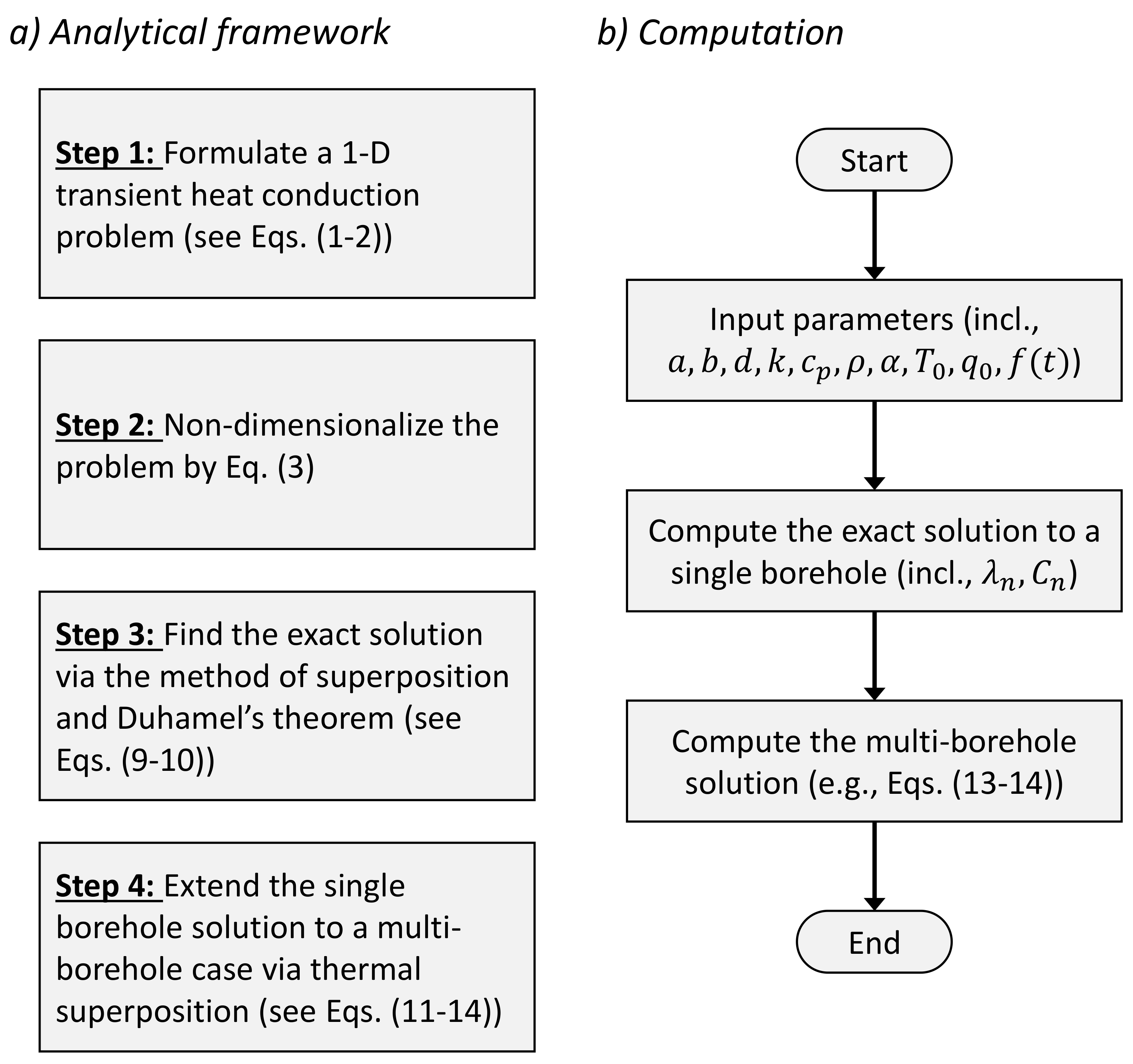
2. Analytical Methods

In a conventional geothermal borehole system (GBS), the BHEs are installed vertically under the ground extracting thermal energy into a heat storage tank, which is then used for spacing heating or other usages. However, in a S-GBS or W-GBS, solar power or waste heat also generates heat and the heat is transported into the heat storage tank as an energy input. In the summer, excess heat can be stored in the ground using the BHEs; in the winter, the stored heat can be extracted for energy use. This process is schematically demonstrated in Figure 1a). When considering a geothermal system with coaxial closed-loop heat exchangers, several borehole arrangements can be categorized: single borehole, double boreholes, and multiple boreholes (including 3-by-3 and N-by-N configurations), as schematically shown in Figure 2. For mathematical simplification and engineering utility, the following assumptions are undertaken:
(1)
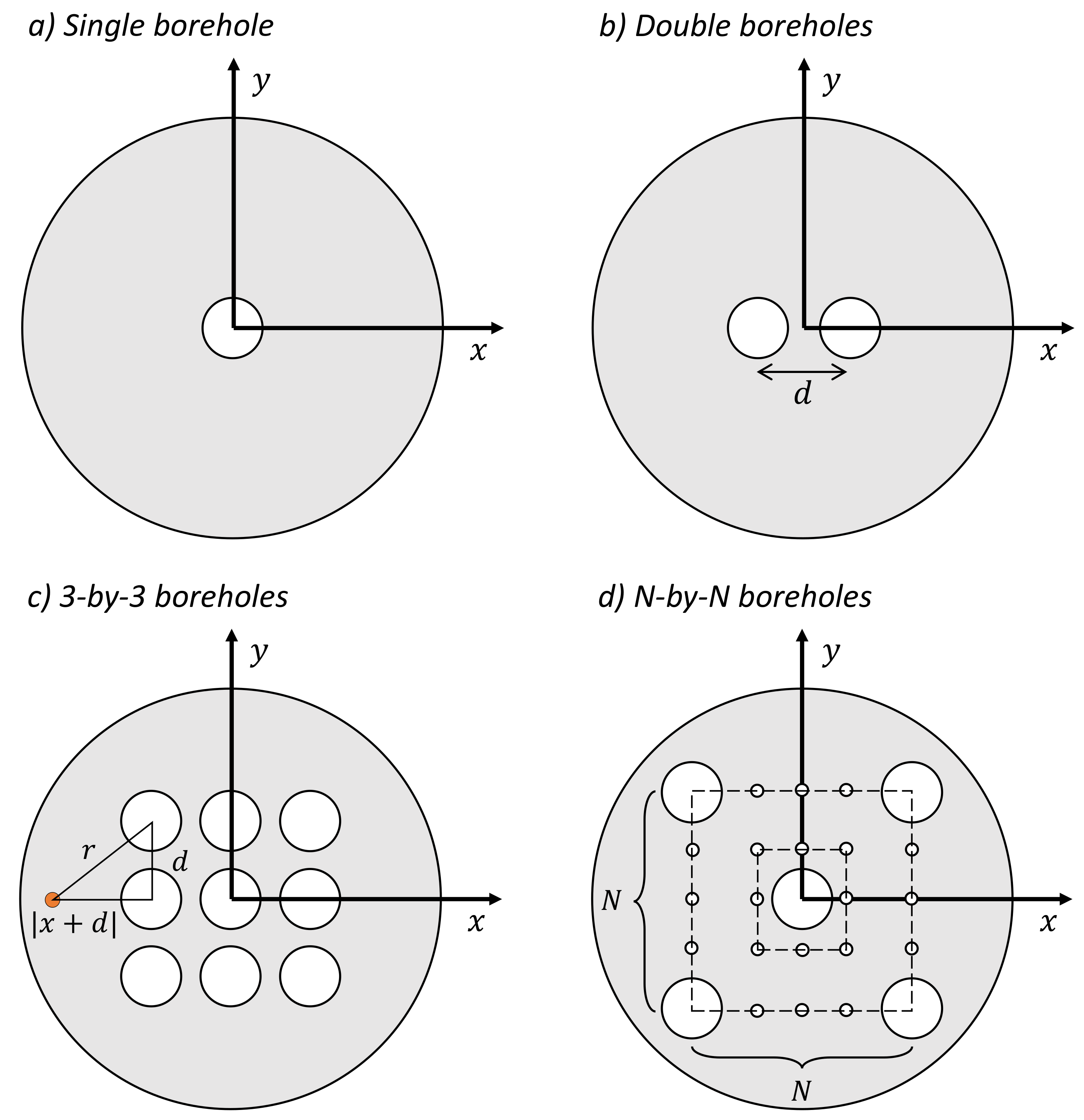
The distance between neighboring boreholes, d [m], are equal in each scenario.
(2)
The boreholes are symmetrically located at the center of the domain (i.e., coaxial heat exchangers).
(3)
The effect of the axial direction in the geothermal system is ignored, which reduces the model to a two-dimensional system in the x- and y-coordinates.
(4)
The conductor pipe in the casing usually has a high thermal conductivity, thus making its thermal resistance negligible.
(5)
The cement/grout filled in the casing assumes to have the same order of magnitude as the ground in terms of thermophysical properties, so there is no need to consider the cement separately from the ground.
(6)
Thermophysical properties of the grout are assumed to be constant, since the temperature variation gives minimal influences on the properties.
Further, a step-by-step summary of the analytical framework is demonstrated in Figure 3a), which will be thoroughly explained in the following subsections.

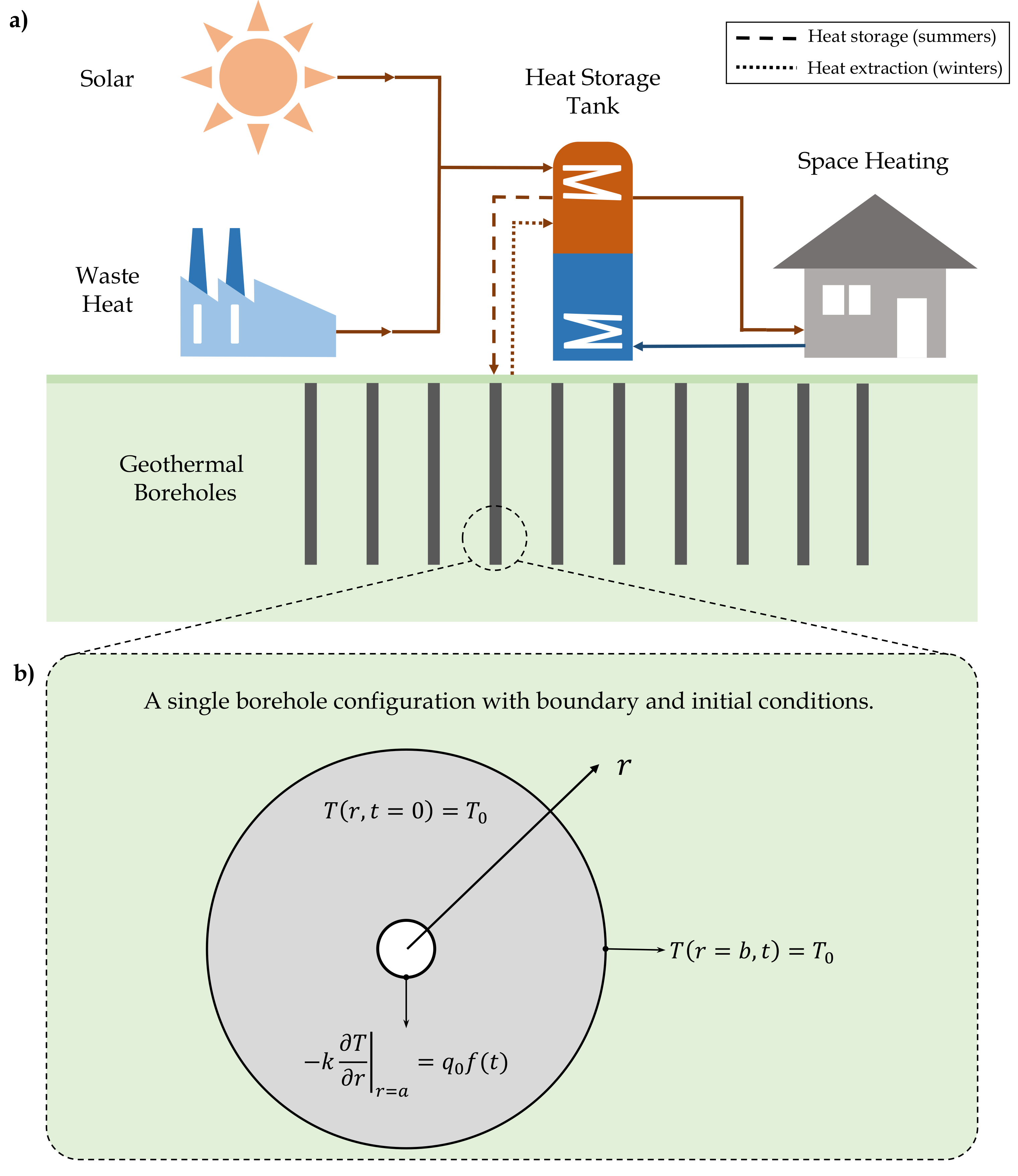
2.1. Problem Formulation

We begin with solving a single borehole scenario, as schematically shown in Figure 1b). In this case, a one-dimensional cylindrical heat conduction model can represent the problem with a governing equation as follows:
2 T r 2 + 1 r T r = 1 α T t ,
where T is the ground temperature (K), r is the radial coordinate (m), t is the time (s), and α is the thermal diffusivity of the ground (m 2 /s). Here, the spatial and temporal domains are a < r < b and t > 0 , respectively. a is the inner radius (m) and b is the outer radius (m). This heat conduction problem is subjected to the following boundary conditions and initial condition:
k T r | r = a = q 0 f ( t ) , T ( r = b , t ) = T 0 , T ( r , t = 0 ) = T 0 ,
where k and T 0 are the thermal conductivity (W/(m·K)) and temperature at the initial and outer boundaries (K), respectively. The initial (and outer) temperature T 0 is also seen as the undisturbed temperature of the ground (K). The heat flux boundary is expressed as q 0 f ( t ) that can be any function of time t, where q 0 represents a constant heat flux (W); if f does not depend on time (i.e., f ( t ) = 1 ), then the boundary reduces to a constant heat flux condition, k ( T / r ) r = a = q 0 .

2.2. Dimensionless Analysis

Prior to conducting mathematical treatments, it is essential to bring the dimensional problem to a non-dimensional form for the purpose of generalization and simplification. We introduce the following dimensionless variables and parameters:
ξ = r a , β = b a , θ = T T 0 q 0 a / k , τ = α t a 2 .
The dimensionless problem is therefore expressed as:
2 θ ξ 2 + θ ξ = θ τ , θ ξ | ξ = 1 = f ( τ ) = F ( τ ) , θ ( β , τ ) = 0 , θ ( ξ , 0 ) = 0 .
Note that f ( τ ) is the dimensionless form of f ( t ) and the negative sign carries from the left-hand side; together, they are denoted as F ( τ ) for simplicity. Since one of the boundary conditions depends on time, the method of separation of variables cannot be directly applied. Alternative approaches are required to convert the time-dependent boundary to a constant one.

2.3. Use of Duhamel’s Theorem

A remedy to deal with linear partial differential equations (e.g., heat equations) subjected to a non-homogeneous time-dependent boundary and/or heat generation is the use of Duhamel’s theorem. The main thrust of this theorem is to solve an auxiliary problem with a time-independent condition reduced from the original formulation, and then integrate it over a desired time interval. This integration term is also known as the Duhamel’s superposition integral. The exact solution to our problem by using the Duhamel’s theorem is expressed as:
θ ( ξ , τ ) = τ ˜ = 0 τ F ( τ ˜ ) Φ ( ξ , τ τ ˜ ) τ d τ ˜ ,
where Φ ( ξ , τ ) is the temperature function in the auxiliary problem and τ ˜ is the time integration variable.
First, the corresponding auxiliary problem is given by:
2 Φ ξ 2 + Φ ξ = Φ τ , Φ ξ | ξ = 1 = 1 , Φ ( β , τ ) = 0 , Φ ( ξ , 0 ) = 0 .
As can be seen, the time-dependent boundary condition is now a constant flux condition. An exact solution is available by the method of superposition consisting of a transient homogeneous partial differential Equation (PDE) and a steady-state second-order ordinary differential Equation (ODE). In fact, this is the same problem as the one subjected to a constant heat flux studied in [39]. Employing the method of superposition, we let Φ ( ξ , τ ) = Φ H ( ξ , τ ) + Φ S S ( ξ ) , where Φ H ( ξ , τ ) is the transient part and Φ S S ( ξ ) is the steady-state term. Consequently, we can obtain the solution to the auxiliary problem as follows:
Φ ( ξ , τ ) = n = 1 C n J 0 ( λ n ξ ) Y 0 ( λ n β ) J 0 ( λ n β ) Y 0 ( λ n ξ ) × exp ( λ n 2 τ ) + ln ξ β ,
where the eigenvalues λ n and the corresponding eigencoefficients C n are found as:
J 1 ( λ n ) Y 0 ( λ n β ) J 0 ( λ n β ) Y 1 ( λ n ) = 0 , n = 1 , 2 , 3 , . . . C n = ξ = 1 β ln ( ξ / β ) ξ [ J 0 ( λ n ξ ) Y 0 ( λ n β ) J 0 ( λ n β ) Y 0 ( λ n ξ ) ] d ξ ξ = 1 β ξ [ J 0 ( λ n ξ ) Y 0 ( λ n β ) J 0 ( λ n β ) Y 0 ( λ n ξ ) ] 2 d ξ .
Last, the exact solution of θ by the Duhamel’s theorem is calculated by substituting Φ into Equation (5). The final expression of θ is
θ ( ξ , τ ) = n = 1 C n λ n 2 exp ( λ n 2 τ ) × J 0 ( λ n ξ ) Y 0 ( λ n β ) J 0 ( λ n β ) Y 0 ( λ n ξ ) × τ ˜ = 0 τ F ( τ ˜ ) exp ( λ n 2 τ ˜ ) d τ ˜ ,
where the eigenvalues λ n and eigencoefficients C n are given in Equation (8). It is worthwhile mentioning the computation of λ n and C n , since the number of terms and precision computed can affect the computational cost and accuracy. The choice of the number and precision of eigenvalues is an iterative process and depends on the problem geometry β . Generally, a rule-of-thumb procedure is to compute more eigen-terms and higher precision and to ensure that the overall temperature solution remains the same.
Another remark is the computation of the integration term, τ ˜ = 0 τ F ( τ ˜ ) exp ( λ n 2 τ ˜ ) d τ ˜ . If the prescribed boundary f ( t ) is a smooth function, e.g., sinusoidal functions, then this integration term can be simplified analytically; however, if f ( t ) is taken as discrete data points over time, then a numerical integration is required, which can be seen as a versatile approach for engineering applications. With modern programming environments, such numerical integration costs very little computational time and power. The final expression of dimensionless temperature θ ( ξ , τ ) in Equation (9) can also be readily transformed into its dimensional form T ( r , t ) as follows:
T ( r , t ) = T 0 + q 0 a k θ ( ξ , τ ) .

2.4. Use of Symmetry: From Single to Multiple Boreholes

Our developed solution for a single borehole can be extended to multiple boreholes by summing up each and every borehole (a.k.a., thermal superposition), as long as the borholes are placed in a symmetrical configuration, as seen in Figure 2. Note that “thermal superposition” should not be confused with the “method of superposition” in Section 2.3: the former is to add the thermal contribution of each borehole, and the latter is the summation of transient and steady-state parts of a PDE to remove its non-homogeneity. The thermal superposition is generally expressed as:
T t o t a l = i = 1 N t o t a l T i = T 1 + T 2 + T 3 + . . . + T N t o t a l ,
where T t o t a l is the temperature distribution for a total of N t o t a l boreholes. T i represents the temperature of the i-th borehole; the determination of each borehole is based on both the general solution, Equation (10), and its location. In this way, the 1D radial temperature solution for a single borehole builds up a 2D solution for multiple boreholes.
Recall that a few arrangements of boreholes are studied as shown in Figure 2: single borehole, double boreholes, and multiple boreholes (3-by-3 and N-by-N configurations. Setting 3-by-3 boreholes as an example here). In this study, we are particularly interested in calculating the temperature profile along the center line at y = 0 , which is equivalent to the line at x = 0 due to its symmetry. That is, T t o t a l ( x , y = 0 , t ) . T t o t a l is denoted as the temperature profile of all boreholes in the domain.
When there is only one borehole in the system, the total temperature profile along the center line is mirrored at x = 0 . Our previously calculated 1-D radial transient temperature solution can be readily implemented as follows:
T t o t a l ( x , y = 0 , t ) = T 1 ( r = x , t ) ,
where the subscript 1 indicates the first and the only borehole in this scenario.
The case of double boreholes means that two boreholes are placed at the center of the domain with a distance of d apart. The total temperature profile along the center line can be calculated by summing the 1D radial transient temperature solution for each borehole:
T t o t a l ( x , y = 0 , t ) = T 1 ( r = x + d 2 , t ) + T 2 ( r = x d 2 , t ) .
When more than two boreholes are present in the system (e.g., four or nine boreholes), there will be boreholes above and below the center line contributing T t o t a l . Consequently, the Pythagorean theorem needs to be applied for examining the correct radial distance from the upper and lower boreholes. In the case of nine boreholes, we find:
T t o t a l ( x , y = 0 , t ) = T 1 ( r = d 2 + ( x + d ) 2 , t ) + T 2 ( r = d 2 + x 2 , t ) + T 3 ( r = d 2 + ( x d ) 2 , t ) + T 4 ( r = x + d , t ) + T 5 ( r = x , t ) + T 6 ( r = x d , t ) + T 7 ( r = d 2 + ( x + d ) 2 , t ) + T 8 ( r = d 2 + x 2 , t ) + T 9 ( r = d 2 + ( x d ) 2 , t ) = 2 × T 1 ( r = d 2 + ( x + d ) 2 , t ) + T 2 ( r = d 2 + x 2 , t ) + T 3 ( r = d 2 + ( x d ) 2 , t ) + T 4 ( r = x + d , t ) + T 5 ( r = x , t ) + T 6 ( r = x d , t ) .
The boreholes are labeled from the top left corner to the bottom right corner, one row after another. Since the top boreholes (No. 1, 2, 3) and bottom boreholes (No. 7, 8, 9) contribute to the center-line temperature in the same manner, we can double the top ones for simplicity, as expressed in Equation (14).
It is rather clear to observe that the closed-form analytical solutions to single, double, and multiple GBS have simple algebraic expressions, without any requirement of temporal and spatial iterations that usually appear in numerical models. As seen in Equation (13) and Equation (14), increasing the number of boreholes only adds more terms in the thermal superposition, which can be rapidly computed and do not add much computational time or power.

3. Model Development

3.1. S-GBS Models

Solar-assisted geothermal borehole systems (S-GBS) were modeled by using the MATLAB R2021b programming language. The code followed closely with the analytical methods developed previously in Section 2 and summarized in Figure 3. In particular, the computation of a S-GBS was shown as follows:
(i)
Prescribe geometry, thermophysical properties, and time-dependent heat flux boundary of S-GBS;
(ii)
For a single borehole case, compute the exact solution, as expressed in Equation (10), to a 1-D radial transient cylindrical heat conduction problem subjected to a time-dependent heat flux boundary; and
(iii)
For the multiple boreholes case, compute the thermal superposition solution based on Equation (11) after step (ii). The scenarios of double and 3-by-3 boreholes at the center line were given in Equations (13) and (14), respectively.
The geometrical and thermophysical parameters required in the model were listed in Table 1, consistent with the values in [39]. On the other hand, the time-dependent boundary for the S-GHS was typically seen as a sinusoidal function varying from 20 (W/m) to 10 (W/m) over a year period. For one unit depth, this boundary was graphed by the red solid line in Figure 4 and it was expressed as
q = k T r = q 0 f ( t ) = A 0 + n = 1 2 A n cos ( n w t ) + B n sin ( n w t ) ,
where q 0 = 1 and the constants in the Fourier series were: A 0 = 3.574 , A 1 = 14.95 , B 1 = 1.389 , A 2 = 1.478 , B 2 = 0.2771 , w = 1.96 × 10 7 . Note that all the variables are in SI units for consistency.

3.2. W-GBS Models

Waste-heat-assisted geothermal borehole systems (W-GBS) were modeled under the same programming environment and procedure as the S-GBS, except for the time-dependent heat flux boundary. The charging process W-GBS was driven by regenerative burner mechanism, providing a constant heat source throughout the cold seasons. During the warm seasons, the W-GBS discharged the stored heat in the same way as the S-GBS. These charging and discharging processes in W-GBS led to a piece-wise function as demonstrated in Figure 4 and the piece-wise boundary condition was written as
q = k T r = q 0 f ( t ) = A 0 + n = 1 2 A n cos ( n w t ) + B n sin ( n w t ) , t 1 t t 2 20 , 0 < t < t 1 or t 2 < t < t 3
where t 1 , t 2 , t 3 were time thresholds to separate the charging and discharging processes. Their values were found to be 8.17 × 10 6 , 2.36 × 10 7 , 3.15 × 10 7 , respectively.

3.3. Numerical Models

To verify the developed analytical solution, a two-dimensional numerical model was built via a commercial finite-element code (COMSOL Multiphysics 5.6). The transient heat Equation (1) subjected to the initial and boundary conditions in Equation (2) was solved by the finite-element method. All the parameters involved in the numerical simulation remained the same as the ones in the analytical model, as listed in Table 1; two kinds of heat flux boundaries were expressed in Equation (15) for S-GBS models and Equation (16) for W-GBS models. Further, unstructured meshes are used to discretize the computational domain and a mesh independency study is conducted for the three borehole arrangements. The details can be found in Appendix A.
All the above-mentioned three scenarios shown in Figure 2 were studied over a one-year time simulation for demonstrating seasonal changes, i.e., t = 1 (yr), with a uniform time step of 1 (h). For each borehole scenario, temperature distributions over the line y = 0 were recorded at four seasons. That is, spring at t = 3 (mon), summer at t = 6 (mon), fall at t = 9 (mon), and winter at t = 12 (mon).

4. Results and Discussion

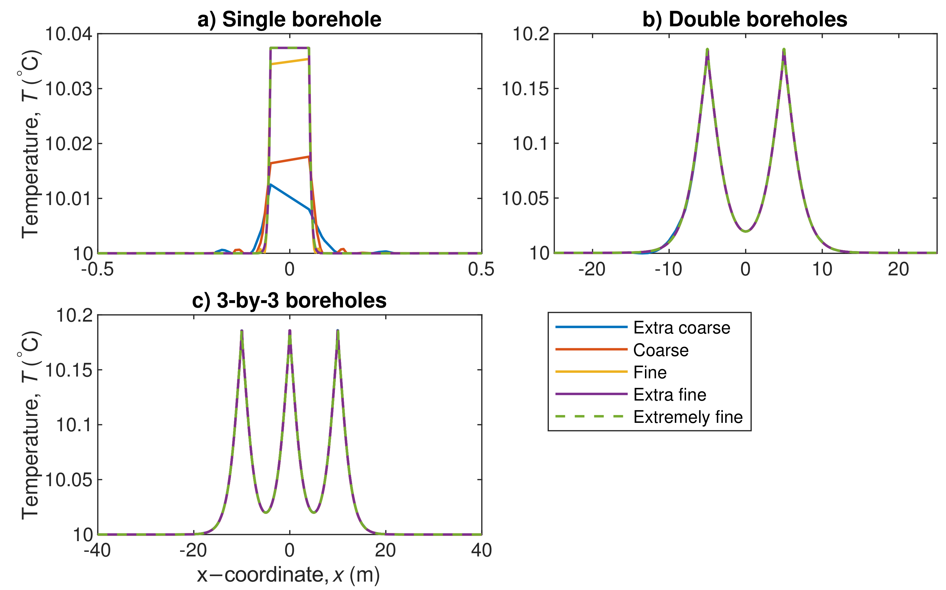
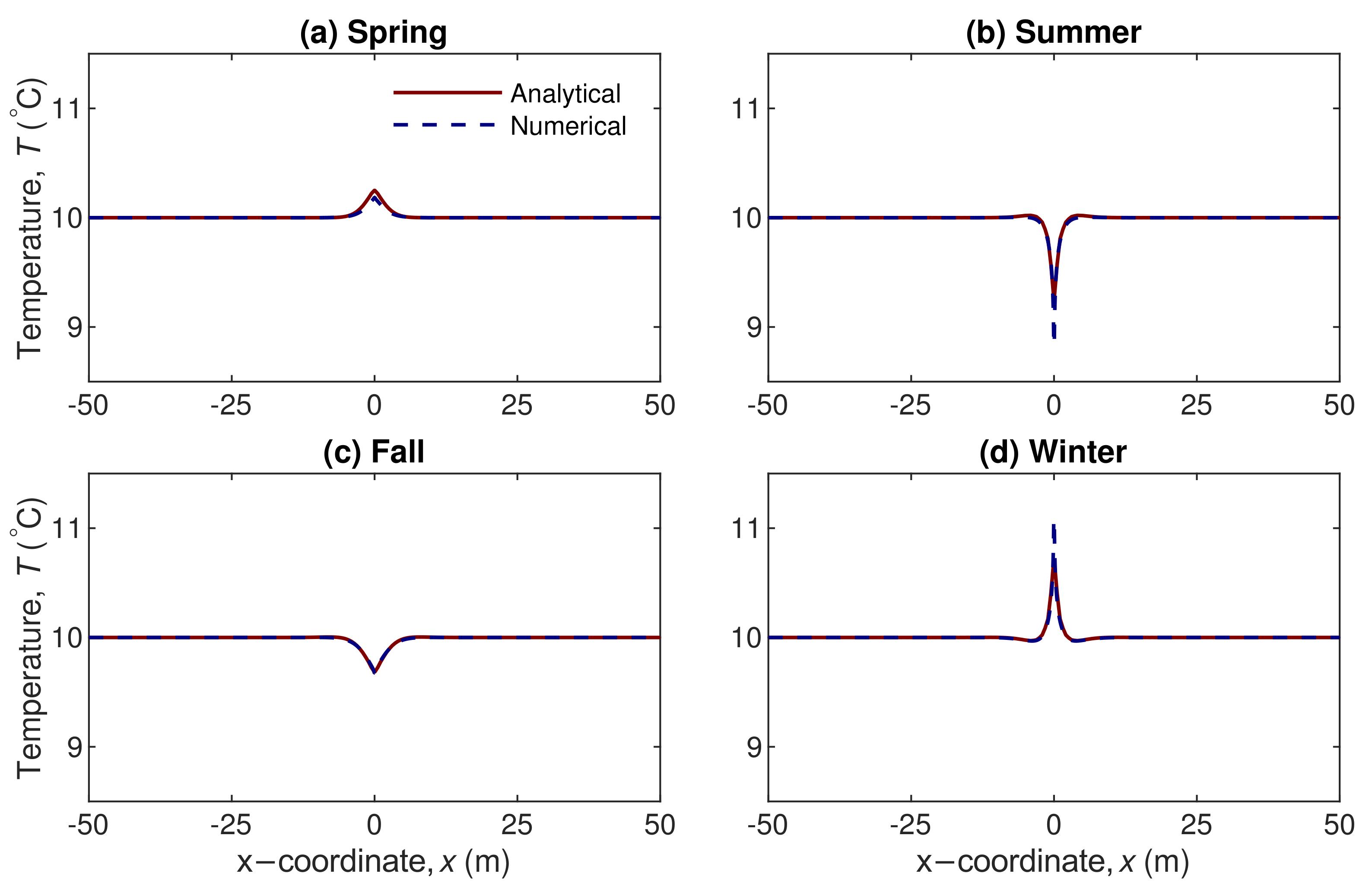
4.1. Model Verification

The developed analytical geothermal borehole model is verified with the numerical results computed by COMSOL. A typical yearly sinusoidal function for seasonal energy storage is prescribed to be the time-dependent boundary condition of an example of geothermal borehole systems; this boundary condition is written as
q = k T r = q 0 f ( t ) = 10 × sin π 15 , 768 , 000 t π 2 ,
where q 0 is set to be 10 (W) and f ( t ) is a sine function. The remaining input parameters, such as thermophysical and geometrical properties, are listed in Table 1. Three borehole configurations are computed in both analytical and numerical methods for verification purposes in the following subsections.

4.1.1. Single Borehole

For the single borehole problem, the temperature distribution over the x-coordinate over four seasons are plotted in Figure 5. The analytical results have an excellent agreement with the numerical data; in particular, the mean absolute deviation (MAD) between the analytical and numerical temperatures ( T a n a l y t i c and T n u m e r i c ) over the x-coordinate with a set of m number of data points can be expressed as:
M A D = 1 m i = 1 m | T a n a l y t i c , i T n u m e r i c , i | .
Based on the four seasons computed in Figure 5, the MAD is found to be minimal falling within the range of 0.0428% to 0.4677%. Meanwhile, the changes in each season are captured, which implies the effect of the time-dependent heat flux. Since the undisturbed temperature ( T 0 ) is at 10 C, the temperature above and below T 0 near the borehole represents the heat supply and extraction over the seasons. In other words, the charging and discharging processes are illustrated in solar-geothermal energy systems. Such temperature differential can convert into energy quantitatively, thus greatly benefiting the economic potential of geothermal systems.

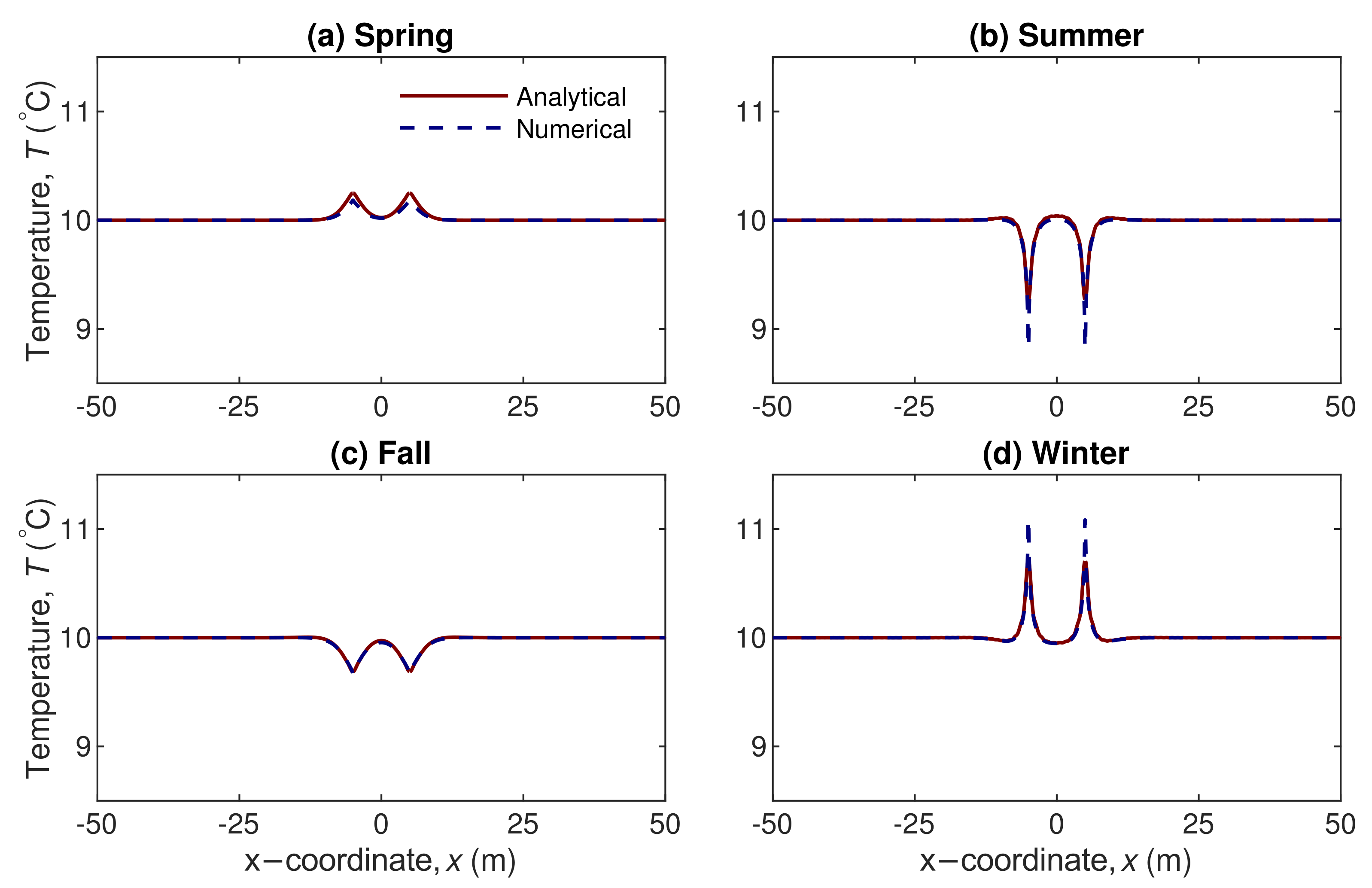
4.1.2. Double and 3-by-3 Boreholes

As per the double boreholes and 3-by-3 boreholes, the temperature profiles are shown in Figure 6 and Figure 7, respectively. A similar agreement of temperature between the analytical and numerical data is found: the MAD range is 0.0568∼0.6115% for double boreholes and 0.0678∼0.6957% for 3-by-3 boreholes. Therefore, there is no significant deviation with numerical data when analytically extending the single borehole into multiple boreholes. The same evolution of temperature is also observed in the multiple boreholes case over four seasons, which leads to a consistent heat supply and extraction processes. It is worthwhile mentioning that the temperature distributions between the neighboring boreholes are well predicted in both cases compared with the numerical results. This agreement represents the success of symmetrical analysis conducted previously in the methodology.

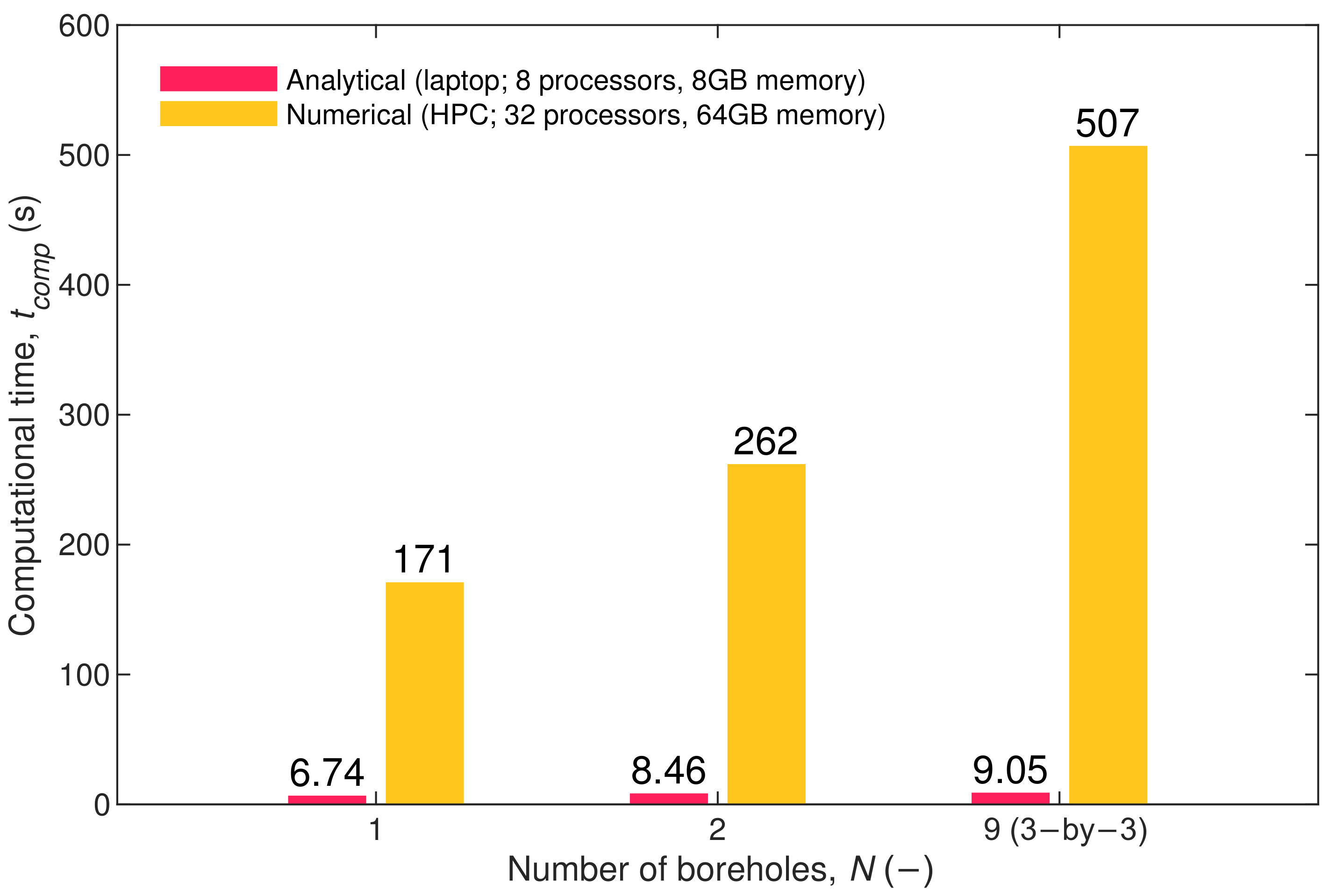
4.1.3. Computational Efficiency

When computing the analytical and numerical models, we find that the analytical computational efficiency (including time and power) is significantly less than the numerical counterpart in all borehole configurations. For the yearly simulation of the geothermal borehole system, the analytical solution (via MATLAB R2021b) takes approximately 6.74 s, 8.46 s, and 9.05 s for the single borehole, double boreholes, and 3-by-3 boreholes, respectively. This analytical algorithm is implemented in a workstation (laptop) of 4 cores, 8 logical processors, and 8 GB of RAM. In contrast, the numerical model built by COMSOL needs 171 s, 262 s, and 507 s in each borehole configuration, respectively, for the same yearly simulation, which is computed under a high performance computing (HPC) workstation using parallel computing with 32 CPUs and 2 GB memory per CPU (64 GB in total). The computational comparison between the analytical and numerical models is demonstrated in Figure 8. It is rather clear to see that our analytical model requires 4∼8 times less of the computational power (regarding both CPUs and total memory) and 24∼55 times less the computational time than the conventional numerical approach.
Another finding is that the computational cost of the numerical model is significantly greater in going from the single to multiple boreholes, yet the analytical solution is not. This is credited to the fact that the analytical solution is done by the linear interpolation in the multiple borehole systems after the exact solution to a single borehole problem is completed. The 2-D numerical model, on the other hand, requires more mesh elements as the number of boreholes increases, and the mesh and time independency studies are needed extensively for each case.

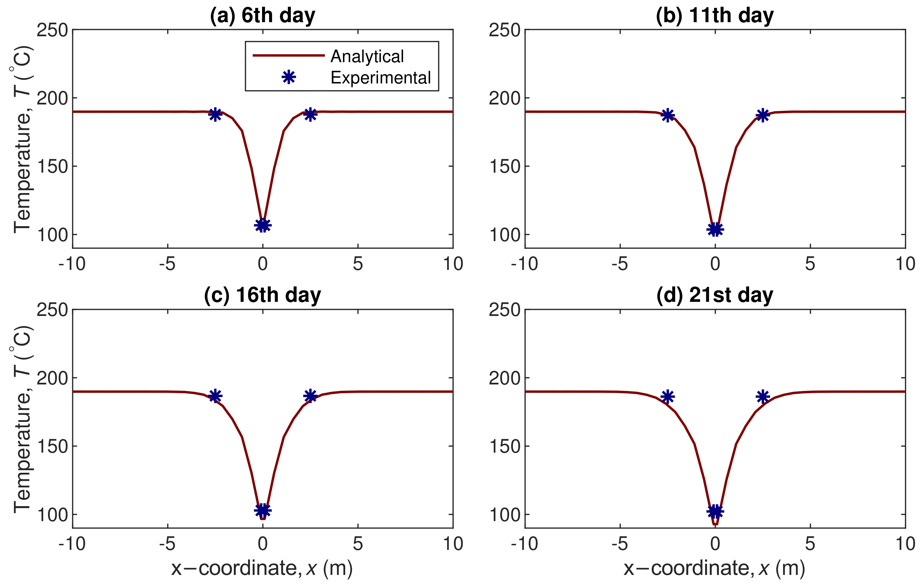
4.2. Model Validation

In addition to the verification with the numerical results, the analytical model is also validated against the experimental data from the literature. Recently, Pokhrel et al. [40] conducted a field-scale experiment of a 500 m coaxial borehole heat exchanger system, and the in situ ground temperature was measured over time. To proceed with the validation against this field-scale experiment, the properties (related to the geometry and thermal physics) and the borehole heat flux are both necessary for the input of our developed analytical model. Firstly, consistent geometrical and thermophysical properties of the ground and working fluid (i.e., water) are prescribed in the analytical model, as listed in Table 2. It is noted that the analytical model only requires the specific heat of the working fluid to calculate the borehole heat flux, and thus there is no need to present other properties in the table here. Secondly, the borehole heat flux is calculated by q = m ˙ c p , w a t e r ( T o u t l e t T i n l e t ) / L , where m ˙ is the mass flow rate of the water ( 1.66 kg/s here), L is the depth (using 250 m since the top half of the borehole is covered by the grout with a relatively high thermal resistance), and T i n l e t and T o u t l e t are the inlet and outlet temperatures ( T i n l e t = 70 C and T o u t l e t is interpolated over time). The borehole heat flux is, therefore, expressed as q = 7.309 × 10 4 t 0.4679 + 713.4 .
Figure 9 shows the validation results regarding the temperature profile at a 400-m depth for four measuring days: the 6th, 11th, 16th, and 21st days. The field-scale experiment has two spatial measurements: one at the borehole ( x = a ), and another one at 2.5 m away ( x = ± 2.5 m). It is rather clear that the developed analytical solution is capable of predicting the temperature around the boreholes with a great validation against the field-scale experiment. The MAD between the analytical solution and the experimental data (here it can be also called the absolute error) is found to be within the range of 0.4727%∼6.2952%.

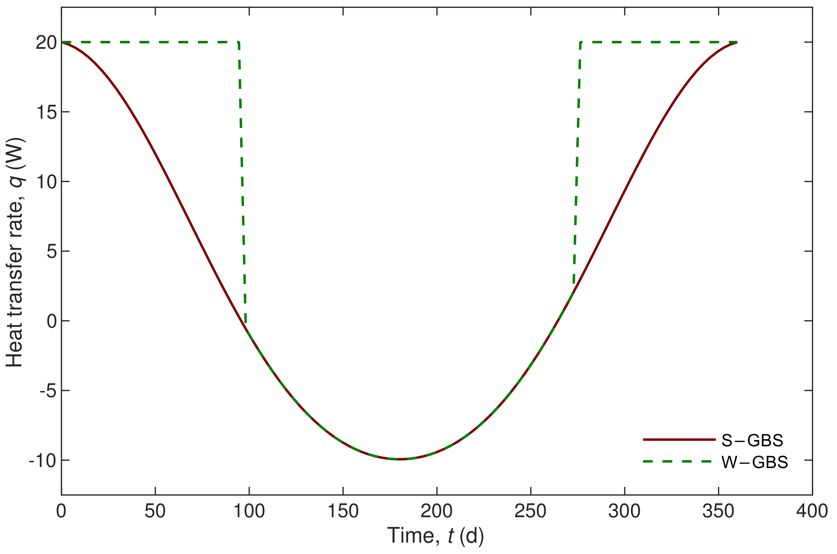
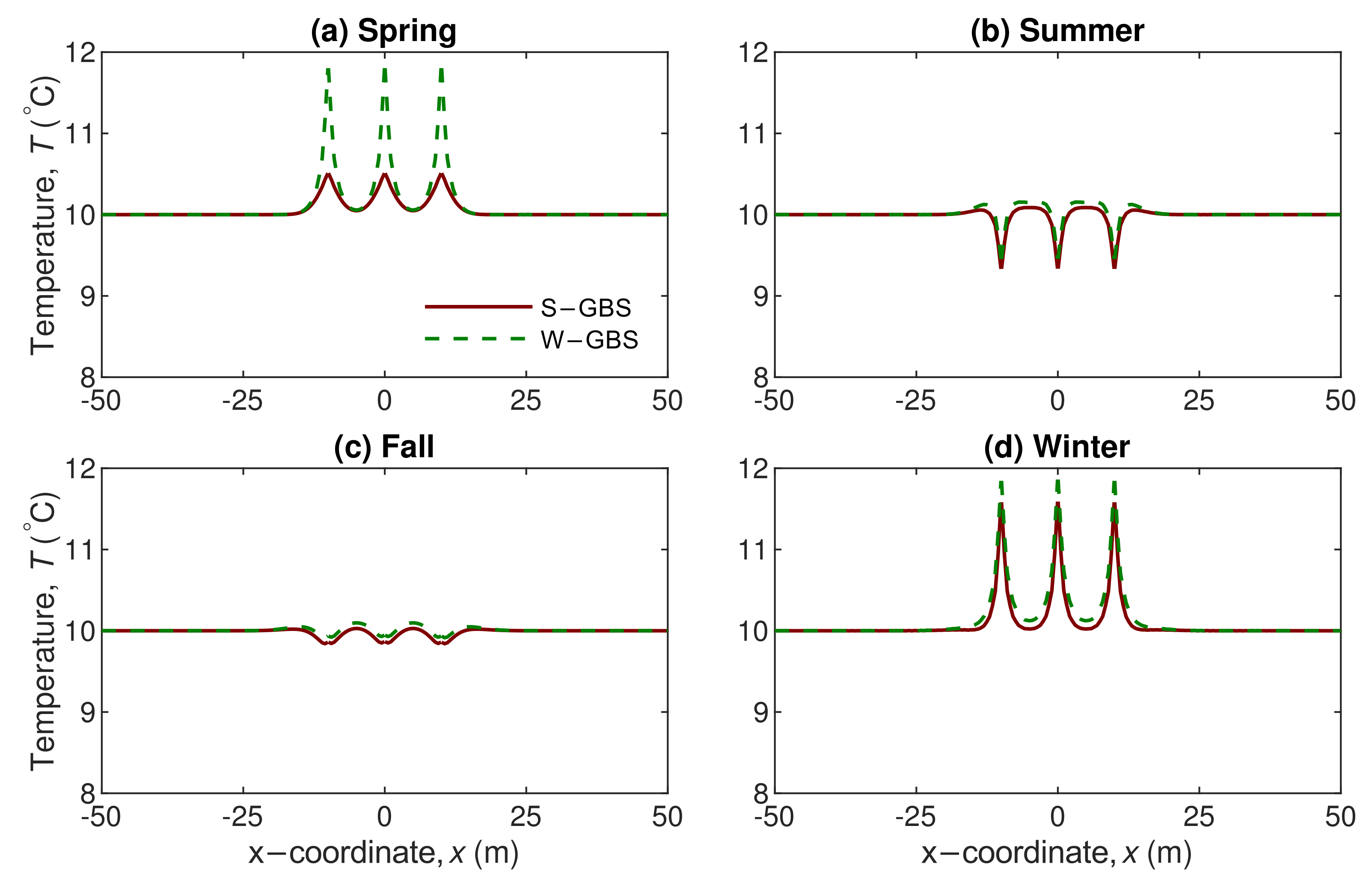
4.3. Comparison between S-GBS and W-GBS

For S-GBS and W-GBS, a comparison is made by computing the 3-by-3 boreholes and the boundary conditions are given by Equations (15) and (16). In this scenario, the charging process is found to be different between the two systems, as shown during the spring and winter seasons in Figure 10. The contrast is particularly significant in the spring, where the near-borehole temperature in W-GBS is around 12% higher than the one in S-GBS. This is caused by the fact that the prescribed time-dependent boundary in W-GBS maintains at a constant heat transfer rate, rather than sinusoidal pattern, throughout the charging period. Although the predefined boundaries are taken in a seasonal resolution (S-GBS at a higher time resolution can have daytime/nighttime fluctuations in colder seasons [33,41]), this comparison still views the energy supply and demand in the two systems. As a result, the W-GBS can generally require more energy input than the S-GBS in terms of the charging process.
As for the discharging time of the year, both systems demonstrate similar behaviors. A slight temperature distribution around the boreholes is observed during summer and fall in Figure 10, which can be explained by the energy residue after the charging process for the W-GBS. Such energy residue is accumulated near each borehole, and it takes time to be distributed to surroundings even after the charging period.

5. Conclusions

The time-dependent boundary condition is of great interest to geothermal borehole systems (including S-GBS and W-GBS), and the corresponding problem in multiple boreholes has profound applications in geothermal borehole systems. This paper proposed an analytical framework of a transient heat conduction problem subjected to a time-dependent boundary from a single borehole to multiple boreholes. The following conclusions and future recommendations were suggested.
(i)
The closed-form analytical solution developed here is verified with a 2-D FEM numerical model (having a mean absolute deviation of below 0.7% in all borehole scenarios) as well as validated against a field-scale experiment in the literature (having an absolute error of below 6.3%) to ensure its accuracy and reliability.
(ii)
The analytical solution is much more computationally efficient to be computed than numerical models, requiring 4∼8 times less computational power and 24∼55 times less computational time.
(ii)
The analytical framework is capable of evaluating the ground temperature in GBS with any time-varying boundary, regardless the number of boreholes. Case studies for S-GBS and W-GBS are also conducted.
(iv)
It was recommended that future studies could consider: the optimal design of borehole spacing and the number of boreholes used; and the economic assessment of such system from the energy demand/supply.

Author Contributions

Conceptualization, M.X., S.A.G.-M. and A.P.S.; methodology, M.X., S.A.G.-M. and A.P.S.; software, M.X.; validation, M.X.; formal analysis, M.X., S.A.G.-M. and A.P.S.; investigation, M.X.; resources, F.H. and A.P.S.; data curation, M.X.; writing—original draft preparation, M.X.; writing—review and editing, M.A.H., F.H., S.A.G.-M., H.M.A., H.A.S., H.A.M.A., G.S.A.H., K.I.A. and A.P.S.; visualization, M.X. and A.P.S.; supervision, A.P.S.; project administration, M.A.H., F.H. and A.P.S.; funding acquisition, M.A.H., S.A.G.-M. and A.P.S. All authors have read and agreed to the published version of the manuscript.

Funding

This research work was funded by the Deputyship for Research & Innovation, Ministry of Education in Saudi Arabia through the project number (IFPRC-091-135-2020) and King Abdulaziz University, DSR, Jeddah, Saudi Arabia.

Institutional Review Board Statement

Not applicable.

Informed Consent Statement

Not applicable.

Data Availability Statement

The data will be made available upon request.

Acknowledgments

The authors extend their appreciation to the Deputyship for Research & Innovation, Ministry of Education in Saudi Arabia for funding this research work through the project number (IFPRC-091-135-2020) and King Abdulaziz University, DSR, Jeddah, Saudi Arabia. Minghan Xu would like to extend his gratitude to McGill Engineering Doctoral Award (MEDA) and Fonds de Recherche du Québec—Nature et Technologies (FRQ-NT) Bourses de maîtrise en recherche (B1X) & Bourse de doctorat en recherche (B2X) for supporting his doctoral study. The numerical simulations for this study were conducted at the HPC facility under Calcul-Québec and Compute-Canada with contribution from CFI-JELF.

Conflicts of Interest

The authors declare no conflict of interest.

Abbreviations

The following abbreviations are used in this manuscript:
BHEBorehole heat exchanger
CFDComputational fluid dynamics
FEMFinite-element method
HPCHigh performance computing
MADMean absolute deviation
ODEOrdinary differential equation
GSHPGround-source heat pump
PDEPartial differential equation
S-GBSSolar-assisted geothermal borehole system
W-GBSWaste-heat-assisted geothermal borehole system

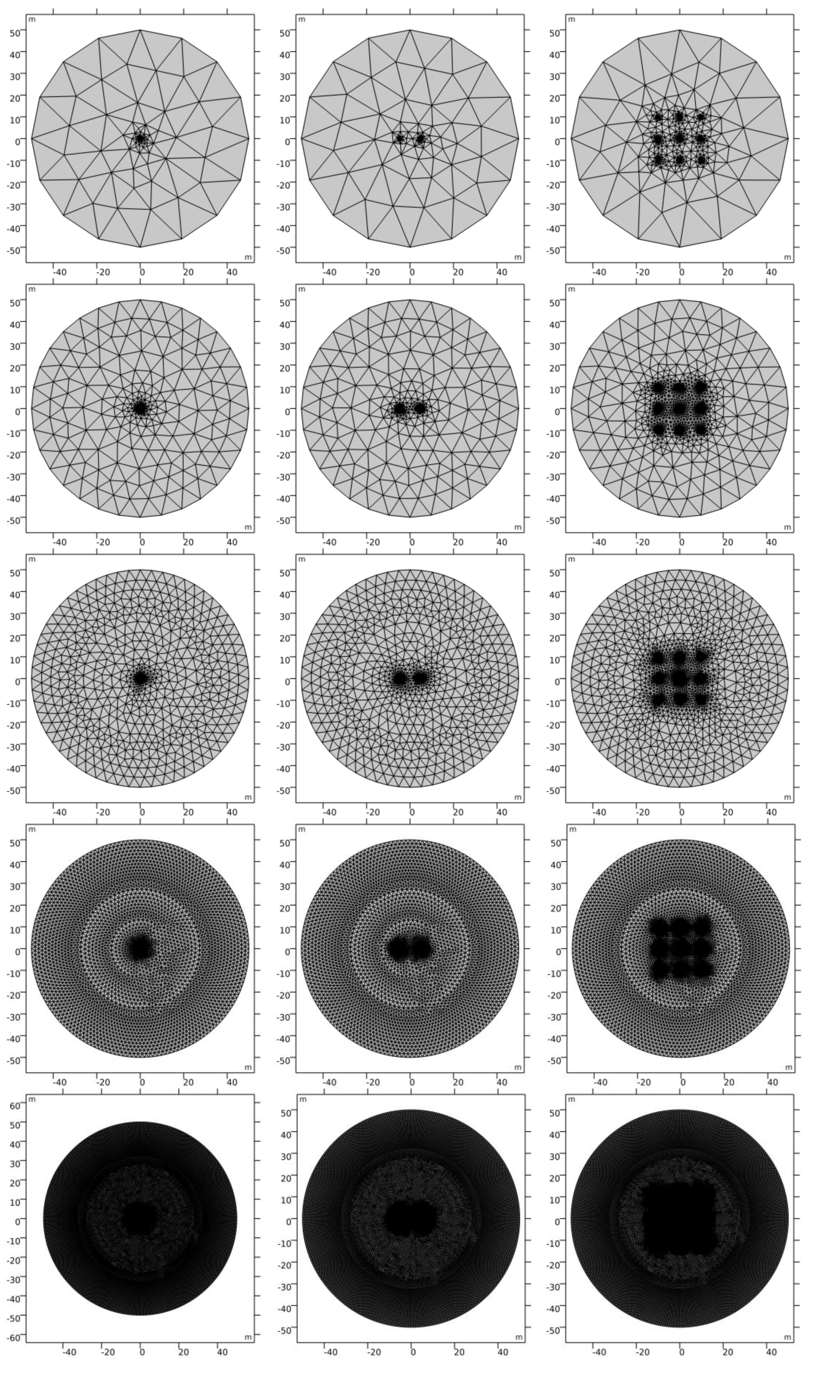
Appendix A. Mesh Type and Mesh Independency Study in the Numerical Models

The unstructured mesh is used to discretize the computational domain, with a refinement near the borehole due to its geometry and the prescribed heat flux boundary condition. The mesh independency study for the 2-dimensional numerical model is also conducted. To ensure the appropriate number of mesh elements, five different mesh counts are selected from coarse to fine as listed in Table A1 and demonstrated in Figure A2.
Table A1. Number of mesh elements for various borehole arrangements and mesh refinements.
Single BoreholeDouble Boreholes3-by-3 Boreholes
Extra coarse2203721580
Coarse69210564293
Fine2012316210,832
Extra fine951612,29031,578
Extremely fine33,83441,24493,672
Figure A1. Temperature distribution over the x-coordinate (i.e., the line y = 0 ) for single, double, and 3-by-3 boreholes in spring ( t = 3 (mon)) for different mesh counts.
Applsci 11 10338 g0a1
Figure A1 shows the temperature distribution over the x-coordinate (i.e., the line y = 0 ) for single, double, and 3-by-3 boreholes in spring ( t = 3 (mon)) with the five numbers of mesh elements. As can be seen, inconsistent results are found in the three coarser mesh counts (that is, extra coarse, coarse, and fine), particularly in the single borehole scenario. However, the temperature distribution of all the three borehole arrangements remains the same while discretizing the domain with the two finer meshes (that is, extra fine and extremely fine). As a consequence, the extra fine option is selected to be the optimal mesh count for this study.
Figure A2. Unstructured mesh scenarios used: extra coarse, coarse, fine, extra fine, extremely fine (from up to bottom); single borehole, double boreholes, 3-by-3 boreholes (from left to right).
Applsci 11 10338 g0a2

References

  1. Templeton, J.D.; Ghoreishi-Madiseh, S.A.; Hassani, F.; Al-Khawaja, M.J. Abandoned petroleum wells as sustainable sources of geothermal energy. Energy 2014, 70, 366–373. [Google Scholar] [CrossRef]
  2. Moya, D.; Aldás, C.; Kaparaju, P. Geothermal energy: Power plant technology and direct heat applications. Renew. Sustain. Energy Rev. 2018, 94, 889–901. [Google Scholar] [CrossRef]
  3. Lund, J.W.; Toth, A.N. Direct utilization of geothermal energy 2020 worldwide review. Geothermics 2020, 90, 101915. [Google Scholar] [CrossRef]
  4. Lund, J.W.; Boyd, T.L. Direct utilization of geothermal energy 2015 worldwide review. Geothermics 2016, 60, 66–93. [Google Scholar] [CrossRef]
  5. Dehghani-Sanij, A.; Jatin, N. New trends in enhanced, hybrid and integrated geothermal Systems. Appl. Sci. 2021, 11, 3765. [Google Scholar] [CrossRef]
  6. Ghoreishi-Madiseh, S.A.; Hassani, F.; Abbasy, F. Numerical and experimental study of geothermal heat extraction from backfilled mine stopes. Appl. Therm. Eng. 2015, 90, 1119–1130. [Google Scholar] [CrossRef]
  7. Templeton, J.D.; Ghoreishi-Madiseh, S.A.; Hassani, F.P.; Sasmito, A.P.; Kurnia, J.C. Numerical and experimental study of transient conjugate heat transfer in helical closed-loop geothermal heat exchangers for application of thermal energy storage in backfilled mine stopes. Int. J. Energy Res. 2020, 44, 9609–9616. [Google Scholar] [CrossRef]
  8. Fong, M.; Alzoubi, M.A.; Kurnia, J.C.; Sasmito, A.P. On the performance of ground coupled seasonal thermal energy storage for heating and cooling: A Canadian context. Appl. Energy 2019, 250, 593–604. [Google Scholar] [CrossRef]
  9. Amiri, L.; Madadian, E.; Hassani, F.P. Energo-and exergo-technical assessment of ground-source heat pump systems for geothermal energy production from underground mines. Environ. Technol. 2019, 40, 3534–3546. [Google Scholar] [CrossRef]
  10. Cui, Y.; Zhu, J.; Twaha, S.; Chu, J.; Bai, H.; Huang, K.; Chen, X.; Zoras, S.; Soleimani, Z. Techno-economic assessment of the horizontal geothermal heat pump systems: A comprehensive review. Energy Convers. Manag. 2019, 191, 208–236. [Google Scholar] [CrossRef]
  11. Kurnia, J.C.; Shatri, M.S.; Putra, Z.A.; Zaini, J.; Caesarendra, W.; Sasmito, A.P. Geothermal energy extraction using abandoned oil and gas wells: Techno-economic and policy review. Int. J. Energy Res. 2021, 1–33. [Google Scholar] [CrossRef]
  12. Kurnia, J.C.; Putra, Z.A.; Muraza, O.; Ghoreishi-Madiseh, S.A.; Sasmito, A.P. Numerical evaluation, process design and techno-economic analysis of geothermal energy extraction from abandoned oil wells in Malaysia. Renew. Energy 2021, 175, 868–879. [Google Scholar] [CrossRef]
  13. Lamarche, L.; Kajl, S.; Beauchamp, B. A review of methods to evaluate borehole thermal resistances in geothermal heat-pump systems. Geothermics 2010, 39, 187–200. [Google Scholar] [CrossRef]
  14. Yang, H.; Cui, P.; Fang, Z. Vertical-borehole ground-coupled heat pumps: A review of models and systems. Appl. Energy 2010, 87, 16–27. [Google Scholar] [CrossRef]
  15. Wang, G.; Song, X.; Shi, Y.; Yulong, F.; Yang, R.; Li, J. Comparison of production characteristics of various coaxial closed-loop geothermal systems. Energy Convers. Manag. 2020, 225, 113437. [Google Scholar]
  16. Song, X.; Wang, G.; Shi, Y.; Li, R.; Xu, Z.; Zheng, R.; Wang, Y.; Li, J. Numerical analysis of heat extraction performance of a deep coaxial borehole heat exchanger geothermal system. Energy 2018, 164, 1298–1310. [Google Scholar] [CrossRef]
  17. Zarrella, A.; Scarpa, M.; Carli, M.D. Short time-step performances of coaxial and double U-tube borehole heat exchangers: Modeling and measurements. HVAC R Res. 2011, 17, 959–976. [Google Scholar]
  18. Acuña, J.; Palm, B. Distributed thermal response tests on pipe-in-pipe borehole heat exchangers. Appl. Energy 2013, 109, 312–320. [Google Scholar]
  19. Bouhacina, B.; Saim, R.; Oztop, H.F. Numerical investigation of a novel tube design for the geothermal borehole heat exchanger. Appl. Therm. Eng. 2015, 79, 153–162. [Google Scholar] [CrossRef]
  20. Gustafsson, A.M.; Westerlund, L.; Hellström, G. CFD-modelling of natural convection in a groundwater-filled borehole heat exchanger. Appl. Therm. Eng. 2010, 30, 683–691. [Google Scholar] [CrossRef] [Green Version]
  21. Iry, S.; Rafee, R. Transient numerical simulation of the coaxial borehole heat exchanger with the different diameters ratio. Geothermics 2019, 77, 158–165. [Google Scholar] [CrossRef]
  22. Khalajzadeh, V.; Heidarinejad, G.; Srebric, J. Parameters optimization of a vertical ground heat exchanger based on response surface methodology. Energy Build. 2011, 43, 1288–1294. [Google Scholar] [CrossRef]
  23. Al-Khoury, R.; Bonnier, P.G.; Brinkgreve, R.B.J. Efficient finite element formulation for geothermal heating systems. Part I: Steady state. Int. J. Num. Methods Eng. 2005, 63, 988–1013. [Google Scholar] [CrossRef]
  24. Al-Khoury, R.; Bonnier, P.G. Efficient finite element formulation for geothermal heating systems. Part II: Transient. Int. J. Num. Methods Eng. 2006, 67, 725–745. [Google Scholar] [CrossRef]
  25. Yu, X.; Li, H.; Yao, S.; Nielsen, V.; Heller, A. Development of an efficient numerical model and analysis of heat transfer performance for borehole heat exchanger. Renew. Energy 2020, 152, 189–197. [Google Scholar] [CrossRef]
  26. Ozudogru, T.Y.; Olgun, C.G.; Senol, A. 3D numerical modeling of vertical geothermal heat exchangers. Geothermics 2014, 51, 312–324. [Google Scholar] [CrossRef]
  27. Eskilson, P. Thermal Analysis of Heat Extraction Boreholes. Ph.D. Thesis, University of Lund, Lund, Sweden, 1987. [Google Scholar]
  28. Yavuzturk, C.; Spitler, J.D. A short time step response factor model for vertical ground loop heat exchangers. ASHRAE Trans. 1999, 105, 475–485. [Google Scholar]
  29. Cimmino, M.; Bernier, M.; Adams, F. A contribution towards the determination of g-functions using the finite line source. Appl. Therm. Eng. 2013, 51, 401–412. [Google Scholar] [CrossRef]
  30. Cimmino, M.; Bernier, M. A semi-analytical method to generate g-functions for geothermal bore fields. Int. J. Heat Mass Transf. 2014, 70, 641–650. [Google Scholar] [CrossRef]
  31. Johnsson, J.; Adl-Zarrabi, B. Modelling and evaluation of groundwater filled boreholes subjected to natural convection. Appl. Energy 2019, 253, 113555. [Google Scholar] [CrossRef]
  32. Cimmino, M.; Baliga, B.R.R. A hybrid numerical-semi-analytical method for computer simulations of groundwater flow and heat transfer in geothermal borehole fields. Int. J. Therm. Sci. 2019, 142, 366–378. [Google Scholar] [CrossRef]
  33. Pokhrel, S.; Amiri, L.; Zueter, A.; Poncet, S.; Hassani, F.P.; Sasmito, A.P.; Ghoreishi-Madiseh, S.A. Thermal performance evaluation of integrated solar-geothermal system; a semi-conjugate reduced order numerical model. Appl. Energy 2021, 303, 117676. [Google Scholar] [CrossRef]
  34. Philippe, M.; Bernier, M.; Marchio, D. Validity ranges of three analytical solutions to heat transfer in the vicinity of single boreholes. Geothermics 2009, 38, 407–413. [Google Scholar] [CrossRef]
  35. Lamarche, L.; Beauchamp, B. New solutions for the short-time analysis of geothermal vertical boreholes. Int. J. Heat Mass Transf. 2007, 50, 1408–1419. [Google Scholar] [CrossRef]
  36. Lamarche, L.; Beauchamp, B. A new contribution to the finite line-source model for geothermal boreholes. Energy Build. 2007, 39, 188–198. [Google Scholar] [CrossRef]
  37. Zeng, H.; Diao, N.; Fang, Z. Heat transfer analysis of boreholes in vertical ground heat exchangers. Int. J. Heat Mass Transf. 2003, 46, 4467–4481. [Google Scholar] [CrossRef]
  38. Lamarche, L. Mixed arrangement of multiple input-output borehole systems. Appl. Therm. Eng. 2017, 124, 466–476. [Google Scholar] [CrossRef]
  39. Ghoreishi-Madiseh, S.A.; Kuyuk, A.F.; de Brito, M.A.R. An analytical model for transient heat transfer in ground-coupled heat exchangers of closed-loop geothermal systems. Appl. Therm. Eng. 2019, 150, 696–705. [Google Scholar] [CrossRef]
  40. Pokhrel, S.; Sasmito, A.P.; Sainoki, A.; Tosha, T.; Tanaka, T.; Nagai, C.; Ghoreishi-Madiseh, S.A. Field-scale experimental and numerical analysis of a downhole coaxial heat exchanger for geothermal energy production. Renew. Energy 2022, 157, 227–246. [Google Scholar]
  41. Cimmino, M.; Eslami-Nejad, P. A simulation model for solar assisted shallow ground heat exchangers in series arrangement. Energy Build. 2017, 182, 521–535. [Google Scholar] [CrossRef]
Figure 1. Schematic diagram of (a) a S-GBS or W-GBS; and (b) a single borehole system with boundary and initial conditions.
Applsci 11 10338 g001
Figure 2. Schematic diagram of different scenarios of borehole systems: (a) single borehole; (b) double boreholes; (c) 3-by-3 boreholes; and (d) N-by-N boreholes.
Applsci 11 10338 g002
Figure 3. Flow chart of: (a) the presented analytical framework and (b) its computation.
Applsci 11 10338 g003
Figure 4. Heat transfer rate q (W) over a year period t (d) for seasonal energy storage in: solar-assisted geothermal borehole systems (S-GBS) and waste-heat-assisted geothermal borehole systems (W-GBS).
Applsci 11 10338 g004
Figure 5. Temperature distribution over the x-coordinate (i.e., the line y = 0 ) for a single borehole over four seasons: (a) Spring ( t = 3 (mon)); (b) Summer ( t = 6 (mon)); (c) Fall ( t = 9 (mon)); and (d) Winter ( t = 12 (mon)). The analytical solution is given by the red solid line and the numerical solution is given by the blue dashed line.
Applsci 11 10338 g005
Figure 6. Temperature distribution over the x-coordinate (i.e., the line y = 0 ) for double boreholes over four seasons: (a) Spring ( t = 3 (mon)); (b) Summer ( t = 6 (mon)); (c) Fall ( t = 9 (mon)); and (d) Winter ( t = 12 (mon)). The analytical solution is given by the red solid line and the numerical solution is given by the blue dashed line.
Applsci 11 10338 g006
Figure 7. Temperature distribution over the x-coordinate (i.e., the line y = 0 ) for 3-by-3 boreholes over four seasons: (a) Spring ( t = 3 (mon)); (b) Summer ( t = 6 (mon)); (c) Fall ( t = 9 (mon)); and (d) Winter ( t = 12 (mon)). The analytical solution is given by the red solid line and the numerical solution is given by the blue dashed line.
Applsci 11 10338 g007
Figure 8. Comparison of computation between the analytical and numerical models.
Applsci 11 10338 g008
Figure 9. Comparisons between the analytical model and the field-scale experimental data from [40] regarding the temperature profile at a depth of 400 m.
Applsci 11 10338 g009
Figure 10. Temperature distribution over the x-coordinate (i.e., the line y = 0 ) for 3-by-3 boreholes over four seasons: (a) Spring ( t = 3 (mon)); (b) Summer ( t = 6 (mon)); (c) Fall ( t = 9 (mon)); and (d) Winter ( t = 12 (mon)). The S-GBS is given by the red solid line and the W-GBS is given by the green dashed line.
Applsci 11 10338 g010
Table 1. Prescribed geometrical and thermophysical parameters of the ground. The listed values of parameters are consistent with the work [39].
ParameterValueUnit
Inner radius, a0.05m
Outer radius, b50m
Distance between neighboring boreholes, d10m
Specific heat, c p 1000J/(kg·K)
Thermal conductivity, k1.5W/(m·K)
Mass density, ρ 2500kg/m 3
Thermal diffusivity, α 5 × 10 7 m 2 /s
Undisturbed temperature, T 0 283.15K
Table 2. Prescribed geometrical and thermophysical parameters of the ground and working fluid (water). The listed values of parameters are consistent with the work [40].
ParameterValueUnit
Inner radius, a0.0889m
Outer radius, b50m
Specific heat (ground), c p , g r o u n d 1100J/(kg·K)
Specific heat (water), c p , w a t e r 4182J/(kg·K)
Thermal conductivity (ground), k g r o u n d 2W/(m·K)
Mass density (ground), ρ g r o u n d 2490kg/m 3
Thermal diffusivity (ground), α g r o u n d 7.3019 × 10 7 m 2 /s
Undisturbed temperature, T 0 463.01K
Publisher’s Note: MDPI stays neutral with regard to jurisdictional claims in published maps and institutional affiliations.

