
Integration of Sentinel-1 and Sentinel-2 Data with the G-SMOTE Technique for Boosting Land Cover Classification Accuracy

 ,
,  ,
,  ,
,  and
and 
Abstract
:1. Introduction
- (1)
- What are the most informative features from Sentinel-1, Sentinel-2, spectral indices, and textural information for LC mapping using three well-known ML algorithms in different landscapes?
- (2)
- What is the performance of the G-SMOTE algorithm in LC classification in different circumstances?
- (3)
- Which ML classifier has higher accuracy on LC mapping at diverse landscapes?
2. Materials
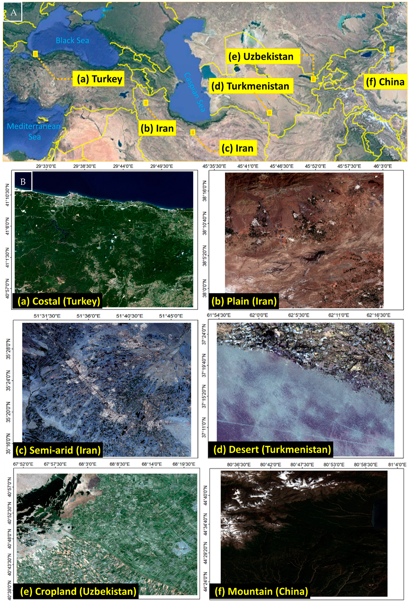
2.1. Overview of the Experiment Sites
2.2. Image and Reference Data
3. Methods
3.1. Methodology
3.2. Spectral and Textural Features
3.3. Feature Selection
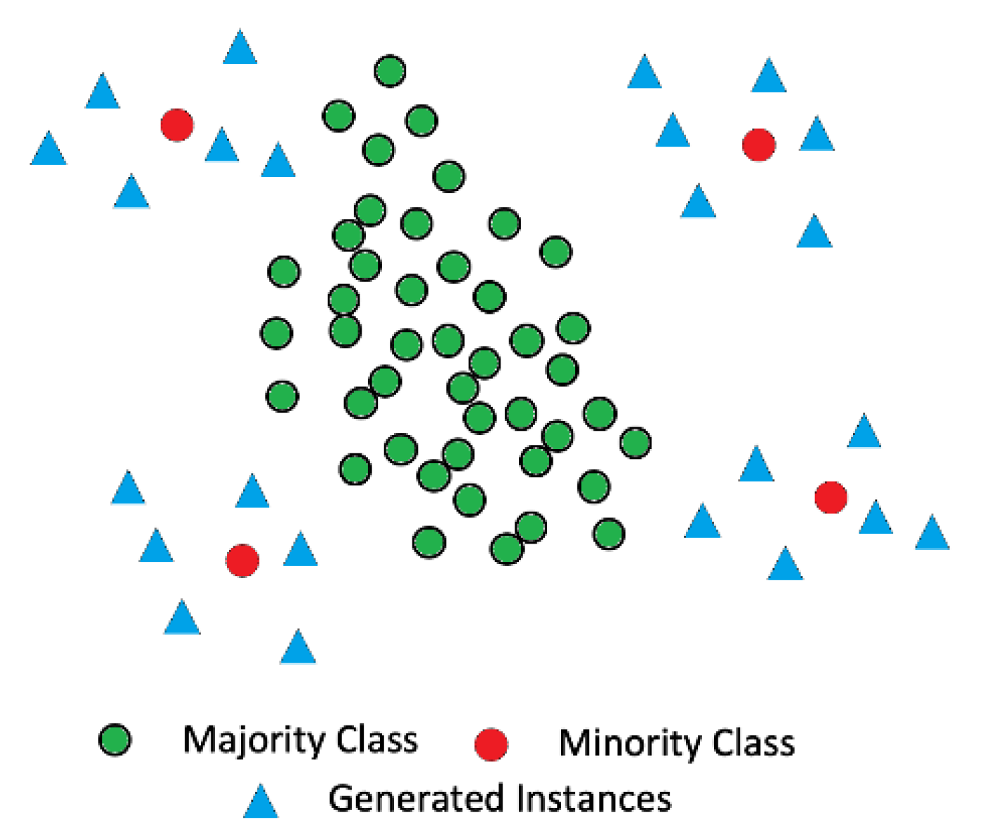
3.4. G-SMOTE
3.5. ML Classifiers and Accuracy Assessment
4. Results

| Methods | SVM | RF | ELM | |||||||
|---|---|---|---|---|---|---|---|---|---|---|
| Sites | Class | UA | PA | OA | UA | PA | OA | UA | PA | OA |
| Coastal | Barren | 0.84 | 0.67 | 0.91 | 0.55 | 0.83 | 0.92 | 0.55 | 0.83 | 0.89 |
| Built-up | 0.85 | 0.75 | 0.93 | 0.65 | 0.83 | 0.75 | ||||
| Cropland | 0.7 | 0.5 | 0.43 | 0.8 | 0.5 | 0.17 | ||||
| Forest | 0.94 | 0.96 | 0.96 | 0.86 | 0.91 | 0.96 | ||||
| Water | 1 | 0.97 | 1 | 1 | 1 | 1 | ||||
| Cropland | Barren | 0.68 | 0.55 | 0.84 | 0.52 | 0.59 | 0.85 | 0.55 | 0.43 | 0.84 |
| Built-up | 0.97 | 0.92 | 0.89 | 0.87 | 0.97 | 0.82 | ||||
| Cropland | 0.87 | 0.96 | 0.83 | 0.9 | 0.82 | 0.92 | ||||
| Pasture | 0.73 | 0.76 | 0.76 | 0.76 | 0.67 | 0.77 | ||||
| Water | 1 | 1 | 1 | 1 | 1 | 1 | ||||
| Desert | Barren | 1 | 1 | 0.94 | 1 | 1 | 0.93 | 1 | 1 | 0.92 |
| Built-up | 0.74 | 0.61 | 0.8 | 0.58 | 0.78 | 0.58 | ||||
| Cropland | 0.9 | 0.99 | 0.8 | 1 | 0.89 | 0.98 | ||||
| Water | 1 | 1 | 1 | 1 | 0.89 | 1 | ||||
| Mountain | Barren | 0.89 | 0.96 | 0.90 | 0.83 | 0.92 | 0.91 | 0.87 | 0.74 | 0.84 |
| Cropland | 0.62 | 0.73 | 0.75 | 0.5 | 0.57 | 0.65 | ||||
| Pasture | 0.96 | 0.84 | 0.91 | 0.87 | 0.81 | 0.91 | ||||
| Snow | 0.9 | 0.9 | 0.81 | 0.81 | 0.73 | 1 | ||||
| Water | 1 | 1 | 1 | 1 | 1 | 1 | ||||
| Plain | Barren | 0.92 | 1 | 0.89 | 0.89 | 0.93 | 0.90 | 0.88 | 1 | 0.89 |
| Built-up | 0.95 | 0.92 | 0.92 | 1 | 0.92 | 0.96 | ||||
| Cropland | 0.88 | 0.91 | 0.89 | 0.91 | 0.88 | 0.91 | ||||
| Pasture | 0.73 | 0.65 | 0.74 | 0.74 | 0.78 | 0.56 | ||||
| Semi-Arid | Barren | 0.82 | 0.91 | 0.84 | 0.86 | 0.89 | 0.85 | 0.82 | 0.85 | 0.84 |
| Built-up | 0.87 | 0.85 | 0.87 | 0.85 | 0.83 | 0.8 | ||||
| Cropland | 0.84 | 0.84 | 0.83 | 0.87 | 0.79 | 0.86 | ||||
| Pasture | 0.57 | 0.53 | 0.55 | 0.57 | 0.53 | 0.56 | ||||
| Methods | SVM | RF | ELM | |||||||
|---|---|---|---|---|---|---|---|---|---|---|
| Sites | Class | UA | PA | OA | UA | PA | OA | UA | PA | OA |
| Coastal | Barren | 0.85 | 0.88 | 0.91 | 0.87 | 0.83 | 0.92 | 0.85 | 0.85 | 0.88 |
| Built-up | 0.88 | 0.76 | 0.84 | 0.80 | 0.84 | 0.75 | ||||
| Cropland | 0.91 | 0.85 | 0.80 | 0.81 | 0.77 | 0.83 | ||||
| Forest | 0.93 | 0.9 | 0.90 | 0.89 | 0.90 | 0.94 | ||||
| Water | 1 | 1 | 1 | 1 | 1 | 1 | ||||
| Cropland | Barren | 0.80 | 0.77 | 0.84 | 0.75 | 0.79 | 0.85 | 0.72 | 0.77 | 0.85 |
| Built-up | 0.93 | 0.90 | 0.87 | 0.85 | 0.89 | 0.80 | ||||
| Cropland | 0.88 | 0.91 | 0.84 | 0.86 | 0.83 | 0.84 | ||||
| Pasture | 0.85 | 0.87 | 0.80 | 0.82 | 0.77 | 0.79 | ||||
| Water | 1 | 1 | 1 | 1 | 1 | 1 | ||||
| Desert | Barren | 1 | 1 | 0.93 | 1 | 0.98 | 0.93.5 | 0.97 | 1 | 0.91 |
| Built-up | 0.88 | 0.78 | 0.89 | 0.79 | 0.79 | 0.87 | ||||
| Cropland | 0.92 | 0.93 | 0.9 | 0.94 | 0.92 | 0.82 | ||||
| Water | 1 | 1 | 1 | 1 | 1 | 1 | ||||
| Mountain | Barren | 0.9 | 0.96 | 0.91 | 0.83 | 0.95 | 0.90 | 0.85 | 0.81 | 0.84 |
| Cropland | 0.85 | 0.82 | 0.85 | 0.88 | 0.80 | 0.78 | ||||
| Pasture | 0.96 | 0.9 | 0.86 | 0.94 | 0.84 | 0.94 | ||||
| Snow | 0.92 | 1 | 0.78 | 0.80 | 0.90 | 0.89 | ||||
| Water | 1 | 1 | 1 | 1 | 1 | 1 | ||||
| Plain | Barren | 0.91 | 0.98 | 0.90 | 0.89 | 0.93 | 0.89 | 0.93 | 0.95 | 0.88 |
| Built-up | 0.92 | 0.92 | 0.93 | 0.95 | 0.92 | 0.92 | ||||
| Cropland | 0.89 | 0.91 | 0.89 | 0.90 | 0.93 | 0.93 | ||||
| Pasture | 0.80 | 0.75 | 0.81 | 0.78 | 0.82 | 0.78 | ||||
| Semi-Arid | Barren | 0.86 | 0.81 | 0.83 | 0.83 | 0.87 | 0.85 | 0.80 | 0.83 | 0.845 |
| Built-up | 0.86 | 0.85 | 0.89 | 0.85 | 0.82 | 0.82 | ||||
| Cropland | 0.82 | 0.83 | 0.80 | 0.85 | 0.80 | 0.83 | ||||
| Pasture | 0.79 | 0.74 | 0.75 | 0.77 | 0.77 | 0.75 | ||||
5. Discussion
5.1. Most Informative Feature
5.2. Comparison of ML Classifiers
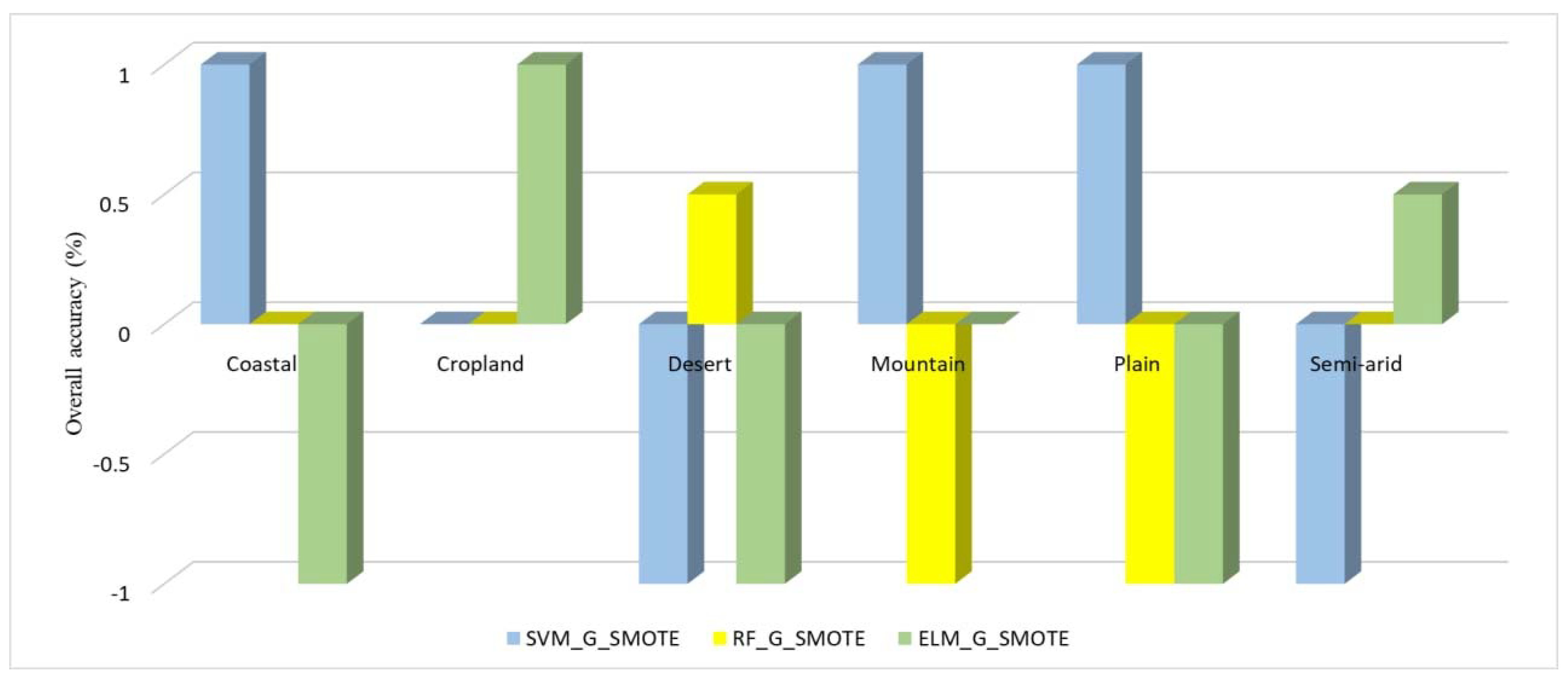
5.3. Effect of G-SMOTE on LC Classification Accuracy
6. Conclusions
Author Contributions
Funding
Institutional Review Board Statement
Informed Consent Statement
Data Availability Statement
Acknowledgments
Conflicts of Interest
References
- Etter, A.; McAlpine, C.; Pullar, D.; Possingham, H. Modelling the conversion of colombian lowland ecosystems since 1940: Drivers, patterns and rates. J. Environ. Manag. 2006, 79, 74–87. [Google Scholar] [CrossRef]
- Moharrami, M.; Naboureh, A.; Gudiyangada Nachappa, T.; Ghorbanzadeh, O.; Guan, X.; Blaschke, T. National-scale landslide susceptibility mapping in austria using fuzzy best-worst multi-criteria decision-making. ISPRS Int. J. Geo-Inf. 2020, 9, 393. [Google Scholar] [CrossRef]
- Ghorbanzadeh, O.; Valizadeh Kamran, K.; Blaschke, T.; Aryal, J.; Naboureh, A.; Einali, J.; Bian, J. Spatial prediction of wildfire susceptibility using field survey gps data and machine learning approaches. Fire 2019, 2, 43. [Google Scholar] [CrossRef] [Green Version]
- Houghton, R.A.; House, J.I.; Pongratz, J.; Van Der Werf, G.R.; DeFries, R.S.; Hansen, M.C.; Quéré, C.L.; Ramankutty, N. Carbon emissions from land use and land-cover change. Biogeosciences 2012, 9, 5125–5142. [Google Scholar] [CrossRef] [Green Version]
- Naboureh, A.; Bian, J.; Lei, G.; Li, A. A review of land use/land cover change mapping in the china-central asia-west asia economic corridor countries. Big Earth Data 2020, 5, 237–257. [Google Scholar] [CrossRef]
- Abdi, A.M. Land cover and land use classification performance of machine learning algorithms in a boreal landscape using sentinel-2 data. GISci. Remote Sens. 2020, 57, 1–20. [Google Scholar] [CrossRef] [Green Version]
- Clerici, N.; Calderón, C.A.V.; Posada, J.M. Fusion of sentinel-1a and sentinel-2a data for land cover mapping: A case study in the lower magdalena region, colombia. J. Maps 2017, 13, 718–726. [Google Scholar] [CrossRef] [Green Version]
- Ienco, D.; Gaetano, R.; Interdonato, R.; Ose, K.; Minh, D.H.T. Combining sentinel-1 and sentinel-2 time series via rnn for object-based land cover classification. In Proceedings of the IGARSS 2019-2019 IEEE International Geoscience and Remote Sensing Symposium, Yokohama, Japan, 28 July–2 August 2019. [Google Scholar]
- Mercier, A.; Betbeder, J.; Rumiano, F.; Baudry, J.; Gond, V.; Blanc, L.; Bourgoin, C.; Cornu, G.; Marchamalo, M.; Poccard-Chapuis, R. Evaluation of sentinel-1 and 2 time series for land cover classification of forest–agriculture mosaics in temperate and tropical landscapes. Remote Sens. 2019, 11, 979. [Google Scholar] [CrossRef] [Green Version]
- Joshi, N.; Baumann, M.; Ehammer, A.; Fensholt, R.; Grogan, K.; Hostert, P.; Jepsen, M.R.; Kuemmerle, T.; Meyfroidt, P.; Mitchard, E.T. A review of the application of optical and radar remote sensing data fusion to land use mapping and monitoring. Remote Sens. 2016, 8, 70. [Google Scholar] [CrossRef] [Green Version]
- Rakwatin, P.; Longépé, N.; Isoguchi, O.; Shimada, M.; Uryu, Y.; Takeuchi, W. Using multiscale texture information from alos palsar to map tropical forest. Int. J. Remote Sens. 2012, 33, 7727–7746. [Google Scholar] [CrossRef]
- Feizizadeh, B. A novel approach of fuzzy dempster–shafer theory for spatial uncertainty analysis and accuracy assessment of object-based image classification. IEEE Geosci. Remote Sens. Lett. 2018, 15, 18–22. [Google Scholar] [CrossRef]
- Al-Fares, W. Historical Land Use/Land Cover Classification Using Remote Sensing; Springer: Amsterdam, The Netherlands, 2013. [Google Scholar]
- Gómez, C.; White, J.C.; Wulder, M.A. Optical remotely sensed time series data for land cover classification: A review. ISPRS J. Photogramm. Remote Sens. 2016, 116, 55–72. [Google Scholar] [CrossRef] [Green Version]
- Naboureh, A.; Moghaddam, M.H.R.; Feizizadeh, B.; Blaschke, T. An integrated object-based image analysis and ca-markov model approach for modeling land use/land cover trends in the sarab plain. Arab. J. Geosci. 2017, 10, 259. [Google Scholar] [CrossRef]
- Ebrahimy, H.; Azadbakht, M. Downscaling modis land surface temperature over a heterogeneous area: An investigation of machine learning techniques, feature selection, and impacts of mixed pixels. Comput. Geosci. 2019, 124, 93–102. [Google Scholar] [CrossRef]
- Tao, Z.; Xin, H.; Wen, D.; Li, J. Urban building density estimation from high-resolution imagery using multiple features and support vector regression. IEEE J. Sel. Top. Appl. Earth Obs. Remote Sens. 2017, 10, 3265–3280. [Google Scholar]
- Mellor, A.; Boukir, S.; Haywood, A.; Jones, S. Exploring issues of training data imbalance and mislabelling on random forest performance for large area land cover classification using the ensemble margin. ISPRS J. Photogramm. Remote Sens. 2015, 105, 155–168. [Google Scholar] [CrossRef]
- Azadbakht, M.; Fraser, C.S.; Khoshelham, K. Synergy of sampling techniques and ensemble classifiers for classification of urban environments using full-waveform lidar data. Int. J. Appl. Earth Obs. Geoinf. 2018, 73, 277–291. [Google Scholar] [CrossRef]
- Naboureh, A.; Li, A.; Bian, J.; Lei, G.; Amani, M. A hybrid data balancing method for classification of imbalanced training data within google earth engine: Case studies from mountainous regions. Remote Sens. 2020, 12, 3301. [Google Scholar] [CrossRef]
- Waldner, F.; Chen, Y.; Lawes, R.; Hochman, Z. Needle in a haystack: Mapping rare and infrequent crops using satellite imagery and data balancing methods. Remote Sens. Environ. 2019, 233, 111375. [Google Scholar] [CrossRef]
- Douzas, G.; Bacao, F. Geometric smote a geometrically enhanced drop-in replacement for smote. Inf. Sci. 2019, 501, 118–135. [Google Scholar] [CrossRef]
- Zha, Y.; Gao, J.; Ni, S. Use of normalized difference built-up index in automatically mapping urban areas from tm imagery. Int. J. Remote Sens. 2003, 24, 583–594. [Google Scholar] [CrossRef]
- Guyon, I.; Weston, J.; Barnhill, S.; Vapnik, V. Gene selection for cancer classification using support vector machines. Mach. Learn. 2002, 46, 389–422. [Google Scholar] [CrossRef]
- Douzas, G.; Bacao, F.; Fonseca, J.; Khudinyan, M. Imbalanced learning in land cover classification: Improving minority classes’ prediction accuracy using the geometric smote algorithm. Remote Sens. 2019, 11, 3040. [Google Scholar] [CrossRef] [Green Version]
- Mountrakis, G.; Im, J.; Ogole, C. Support vector machines in remote sensing: A review. ISPRS J. Photogramm. Remote Sens. 2011, 66, 247–259. [Google Scholar] [CrossRef]
- Tax, D.M.; Duin, R.P. Support vector data description. Mach. Learn. 2004, 54, 45–66. [Google Scholar] [CrossRef] [Green Version]
- Belgiu, M.; Drăguţ, L. Random forest in remote sensing: A review of applications and future directions. ISPRS J. Photogramm. Remote Sens. 2016, 114, 24–31. [Google Scholar] [CrossRef]
- Huang, G.-B.; Zhu, Q.-Y.; Siew, C.-K. Extreme learning machine: Theory and applications. Neurocomputing 2006, 70, 489–501. [Google Scholar] [CrossRef]
- Ghorbanzadeh, O.; Blaschke, T.; Gholamnia, K.; Meena, S.R.; Tiede, D.; Aryal, J. Evaluation of different machine learning methods and deep-learning convolutional neural networks for landslide detection. Remote Sens. 2019, 11, 196. [Google Scholar] [CrossRef] [Green Version]
- Tavakkoli Piralilou, S.; Shahabi, H.; Jarihani, B.; Ghorbanzadeh, O.; Blaschke, T.; Gholamnia, K.; Meena, S.R.; Aryal, J. Landslide detection using multi-scale image segmentation and different machine learning models in the higher himalayas. Remote Sens. 2019, 11, 2575. [Google Scholar] [CrossRef] [Green Version]
- Memarian, H.; Balasundram, S.K.; Talib, J.B.; Sung, C.T.B.; Sood, A.M.; Abbaspour, K. Validation of ca-markov for simulation of land use and cover change in the langat basin, malaysia. J. Geogr. Inf. Syst. 2012, 4, 542–554. [Google Scholar] [CrossRef] [Green Version]
- Pontius, R.G., Jr.; Millones, M. Death to kappa: Birth of quantity disagreement and allocation disagreement for accuracy assessment. Int. J. Remote Sens. 2011, 32, 4407–4429. [Google Scholar] [CrossRef]
- Dong, J.; Xiao, X.; Sheldon, S.; Biradar, C.; Duong, N.D.; Hazarika, M. A comparison of forest cover maps in mainland southeast asia from multiple sources: Palsar, meris, modis and fra. Remote Sens. Environ. 2012, 127, 60–73. [Google Scholar] [CrossRef]
- Tavares, P.A.; Beltrão, N.E.S.; Guimarães, U.S.; Teodoro, A.C. Integration of sentinel-1 and sentinel-2 for classification and lulc mapping in the urban area of belém, eastern brazilian amazon. Sensors 2019, 19, 1140. [Google Scholar] [CrossRef] [PubMed] [Green Version]
- Adam, E.; Mutanga, O.; Odindi, J.; Abdel-Rahman, E.M. Land-use/cover classification in a heterogeneous coastal landscape using RapidEye imagery: Evaluating the performance of random forest and support vector machines classifiers. Int. J. Remote Sens. 2014, 35, 3440–3458. [Google Scholar] [CrossRef]
| Sites | Number of Scenes | |
|---|---|---|
| Sentinel-1 | Sentinel-2 | |
| Coastal | 208 | 146 |
| Cropland | 89 | 145 |
| Desert | 92 | 102 |
| Mountain | 118 | 91 |
| Plain | 118 | 140 |
| Semi-Arid | 117 | 76 |
| Site | Barren | Built-Up | Cropland | Forest | Pasture | Snow | Water |
|---|---|---|---|---|---|---|---|
| Coastal | 196 | 158 | 103 | 218 | - | - | 165 |
| Cropland | 90 | 182 | 249 | - | 93 | - | 89 |
| Desert | 346 | 100 | 264 | - | - | - | 108 |
| Mountain | 355 | - | 97 | - | 321 | 203 | 101 |
| Plain | 234 | 182 | 227 | - | 116 | - | - |
| Semi-Arid | 265 | 234 | 268 | - | 79 | - | - |
| Spectral Index | Formula |
|---|---|
| NDBI | (B11 − B8)/(B11 + B8) |
| NDVI | (B8 − B4)/(B8 + B4) |
| NDWI | (B8 − B3)/(B8 + B3) |
| Sites | Selected Features by SVM-RFE |
|---|---|
| Coastal | VH, VV, B3, B5, B8A, B12, NDVI, NDWI, NDBI |
| Cropland | VH, VV, B2, B4, B7, B8A, B11, NDVI, variance |
| Desert | VV, B8A, B11, B12, NDVI, mean |
| Mountain | VH, VV, B2, B4, B8A, B12, NDVI, variance |
| Plain | VV, B3, B4, B5, B12, NDVI, NDBI, homogeneity, variance |
| Semi-Arid | VV, B2, B4, B5, B12, NDVI, NDBI, mean |
Publisher’s Note: MDPI stays neutral with regard to jurisdictional claims in published maps and institutional affiliations. |
© 2021 by the authors. Licensee MDPI, Basel, Switzerland. This article is an open access article distributed under the terms and conditions of the Creative Commons Attribution (CC BY) license (https://creativecommons.org/licenses/by/4.0/).
Share and Cite
Ebrahimy, H.; Naboureh, A.; Feizizadeh, B.; Aryal, J.; Ghorbanzadeh, O. Integration of Sentinel-1 and Sentinel-2 Data with the G-SMOTE Technique for Boosting Land Cover Classification Accuracy. Appl. Sci. 2021, 11, 10309. https://doi.org/10.3390/app112110309
Ebrahimy H, Naboureh A, Feizizadeh B, Aryal J, Ghorbanzadeh O. Integration of Sentinel-1 and Sentinel-2 Data with the G-SMOTE Technique for Boosting Land Cover Classification Accuracy. Applied Sciences. 2021; 11(21):10309. https://doi.org/10.3390/app112110309
Chicago/Turabian StyleEbrahimy, Hamid, Amin Naboureh, Bakhtiar Feizizadeh, Jagannath Aryal, and Omid Ghorbanzadeh. 2021. "Integration of Sentinel-1 and Sentinel-2 Data with the G-SMOTE Technique for Boosting Land Cover Classification Accuracy" Applied Sciences 11, no. 21: 10309. https://doi.org/10.3390/app112110309
APA StyleEbrahimy, H., Naboureh, A., Feizizadeh, B., Aryal, J., & Ghorbanzadeh, O. (2021). Integration of Sentinel-1 and Sentinel-2 Data with the G-SMOTE Technique for Boosting Land Cover Classification Accuracy. Applied Sciences, 11(21), 10309. https://doi.org/10.3390/app112110309