Abstract
The intelligent recognition of formed elements in microscopic images is a research hotspot. Whether the microscopic image is clear or blurred is the key factor affecting the recognition accuracy. Microscopic images of human feces contain numerous items, such as undigested food, epithelium, bacteria and other formed elements, leading to a complex image composition. Consequently, traditional image quality assessment (IQA) methods cannot accurately assess the quality of fecal microscopic images or even identify the clearest image in the autofocus process. In response to this difficulty, we propose a blind IQA method based on a deep convolutional neural network (CNN), namely GMANet. The gradient information of the microscopic image is introduced into a low-level convolutional layer of the CNN as a mask attention mechanism to force high-level features to pay more attention to sharp regions. Experimental results show that the proposed network has good consistency with human visual properties and can accurately identify the clearest microscopic image in the autofocus process. Our proposed model, trained on fecal microscopic images, can be directly applied to the autofocus process of leucorrhea and blood samples without additional transfer learning. Our study is valuable for the autofocus task of microscopic images with complex compositions.
1. Introduction
Routine stool evaluation is an important means of pathological screening in hospitals. Doctors diagnose whether there is inflammation in the digestive system of a patient by analyzing the compositions of their stool samples via microscopy. With the rapid development of hardware technology and deep learning, the intelligent recognition of formed elements in microscopic images has gradually become a research hotspot [1,2,3]. However, the quality of the microscopic image seriously affects the recognition accuracy. Blurred images can cause inaccurate cell counts. Therefore, this work mainly focuses on human fecal microscopic image quality assessment, and the ultimate goal is to select the clearest image from a group of microscopic images captured in the autofocus process. Furthermore, we hope that the proposed image quality assessment (IQA) method has good consistency with human visual properties and can be applied not only to human fecal microscopic images, but also to human leucorrhea and blood microscopic images.
IQA methods are mainly categorized as full-reference (FR) IQA methods, reduced-reference (RR) IQA methods, and no-reference (NR) IQA methods. FR-IQA methods such as SSIM [4], FSIM [5], and VIF [6] need to utilize pristine images when evaluating the quality of distorted images. Although the image quality scores predicted by these methods are generally consistent with the human visual system (HVS), pristine images are not available in most practical applications, especially for microscopic images. Moreover, NR-IQA methods without reference images are widely used and studied. Traditional NR-IQA methods normally use image information such as gradient [7], entropy [8], edge [9], and phase [10] as a measure. A single category of information is only applicable to a specific degeneration and scene; consequently, some researchers have designed feature extractors that contain multiple types of image information and use machine learning methods to train regression models [11]. With the continuous advancement of deep learning, convolutional neural networks (CNNs) have been applied successfully in the IQA task [12]. The features extracted by a CNN have stronger image representation ability than handcrafted features; therefore, a CNN is more sensitive to image degradation.
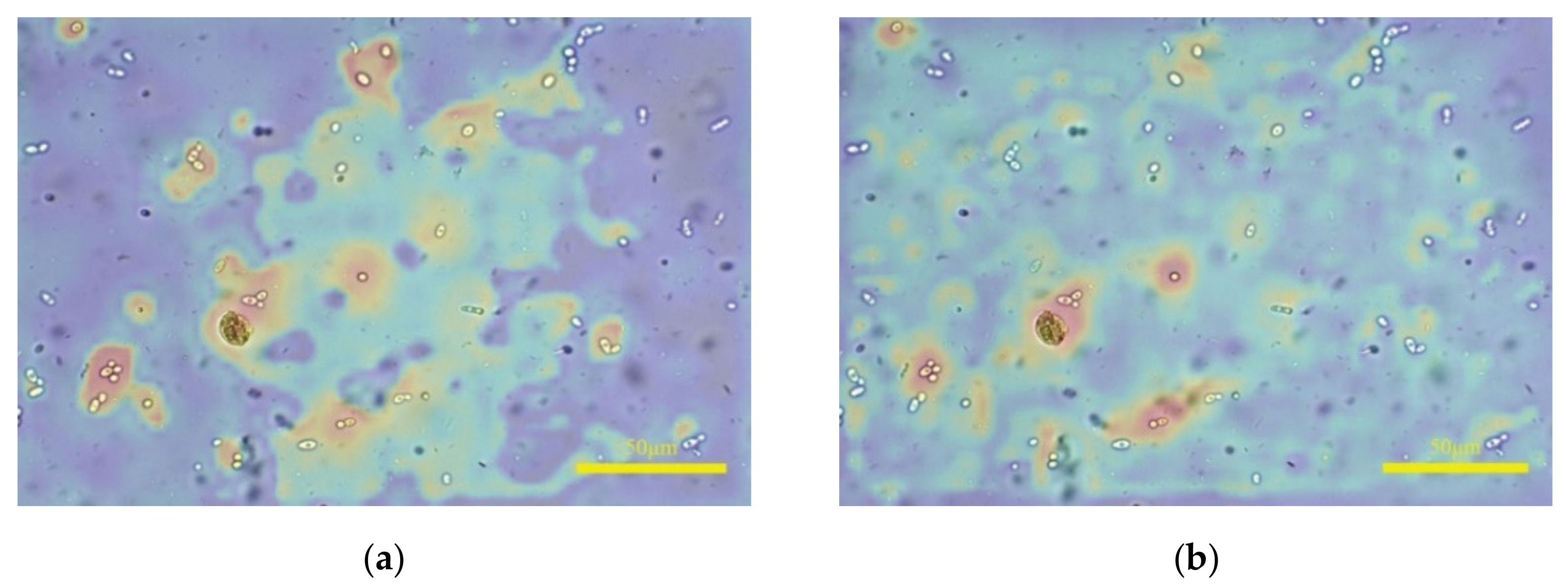
Existing IQA research mainly focuses on how to make algorithm response values more relevant to HVS. The Spearman rank-order correlation coefficient (SROCC) is the most commonly used indicator to evaluate the performance of IQA methods. To verify the effectiveness of a proposed algorithm, many researchers conduct experiments on public databases such as LIVE [13] and TID2013 [14]. The distorted images in these databases are synthetically generated and the degree of degradation is the same everywhere in each distorted image. Compared with public databases, the situations in fecal microscopic images are more complex. On the one hand, the change in fog level is more continuous, and the clarity rating needs to be more refined. On the other hand, human feces contain numerous items, such as undigested food residues, epithelium, and bacteria, and the concentration of substances in different sample solutions is various. Shown in Figure 1a,b are clear microscopic images from a sample solution with low and high concentrations, respectively. Only a small amount of fungal spores is shown in (a), but (b) contains a large amount of particulate matter.
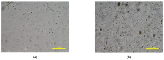
Figure 1.
Complex image composition of fecal microscopic images. (a,b) are clear microscopic images from different feces sample solutions with low and high concentrations, respectively.
A complex image composition leads to clear and blurred areas existing simultaneously in the same fecal microscopic image. During the autofocus process, the response values of captured images rise or fall in oscillation for most traditional IQA methods, yielding multiple extreme points in the response curve. Consequently, it is difficult to assess the quality of a fecal microscopic image or even to identify the clearest image in the autofocus process. In response to the above problems, we proposed a blind IQA method based on a CNN, namely GMANet. Considering that the gradient value of the clear region is greater than that of the blurred region, we introduced the gradient information of the microscopic image into a low-level convolutional layer of the CNN as a mask attention (MA) mechanism to force the high-level features to pay more attention to sharp regions. Our contributions can be summarized as follows:
- We designed a CNN architecture, namely GMANet, which uses gradient information extracted by the local maximum gradient method as an MA mechanism.
- We adopted a feature aggregation module to fuse two low-level feature maps with a high-level feature map and used them to predict quality scores. In the training process, two auxiliary outputs and losses were introduced, which reduces over-fitting and enhances model generality.
- Experimental results show that the GMANet has good consistency with human visual properties and the model trained on fecal microscopic images can be directly applied to the autofocus process of leucorrhea and blood samples without additional transfer learning.
The structure of this paper is as follows: Section 2 introduces some state-of-the-art NR-IQA methods related to this work. The details of the proposed CNN architecture are described in Section 3. Section 4 introduces the materials that we used and the experimental results. Section 5 presents the discussion. Conclusions are provided in Section 6.
2. Related Works
In recent years, deep learning has gradually become a research hotspot among NR-IQA methods. Kang et al. [12] first used a CNN to solve the quality assessment task. In order to meet the need for a large number of training samples for a CNN, they used non-overlapping 32 × 32 patches taken from large images as input and assigned each patch a quality score the same as its source image. The image slicing method has inspired follow-up researchers.
Low-level image information such as gradient is commonly used in traditional IQA methods and can reflect the degree of image distortion. Thus, introducing traditional image information into a CNN can make the predicted score more consistent with HVS. Yan et al. [15] proposed a two-stream convolutional network whose original image and gradient image are input into the network from two branches, respectively. In order to further imitate the operation mode of HVS, some researchers introduced a saliency map into the CNN [16]. Considering that HVS mainly focuses on textured regions rather than flat regions, some researchers studied screening methods for image patches [17,18].
The performance of FR-IQA methods for evaluating image quality is better when comparing the difference between a degraded image and a pristine image. However, pristine images are not available in most practical applications. Thus, some researchers pay attention to how to restore a distorted image to a pristine image by using a generative adversarial network (GAN) [19,20]. Although slicing an image into patches increases the number of training samples, it is easy for a CNN to over-fit on the training dataset due to the small number of pristine images. Therefore, some researchers focus on how to extend the training dataset without additional human labeling work. Liu et al. [21] proposed a Rank-IQA approach that learns from rankings. They used two large public image databases, Waterloo [22] and Places2 [23], and generated synthetic distorted images that were ranked according to their image quality. A pre-trained network was obtained by learning the rank relationship between images in ranked datasets, and then it was fine-tuned on a public IQA database. Guan et al. [24] also used the Waterloo database, and the synthetic distorted images were generated by adding particular levels of distortion to salient and non-salient regions.
For fecal microscopic images, the hypothesis that the quality score of each image patch is the same as its source image is not tenable, as there are both blurred and clear areas in the same image. Considering this, we used a large image patch as the network input and utilized gradient information as the MA mechanism to guide the CNN to pay more attention to clear regions, which is different from other CNN-based IQA methods. In addition, there is no pristine image for a fecal microscopic image; thus, GAN-based IQA methods cannot be used. As the task of this research was to find the clearest image from a group of fecal microscopic images, the theory of learning from rankings used in the Rank-IQA [21] method was adopted in our study.
The goal of existing research is to accurately assess the image quality, but the goal of our paper was to find the clearest image from a group of microscopic images captured in the autofocus process.
3. Method
In this section, we describe the proposed GMANet. The details of the local maximum gradient method is used to extract gradient information are introduced in Section 3.1. The network structure is presented in Section 3.2. Section 3.3 presents the loss function that we used. The training and inference details are provided in Section 3.4.
3.1. Local Maximum Gradient
Xu et al. [25] proposed a deep CNN with an MA mechanism for the classification of COVID-19 from chest X-ray images. They used a segmentation model to predict lung region masks, which were used as a spatial attention map to adjust the features of the classification model. This attention mechanism can suppress the feature value of the background region and improve the classification accuracy. Inspired by this method, we decided to use gradient information as a spatial attention map to suppress the influence of blurred areas. Different from [25], the gradient image was extracted by local maximum gradient method, described below, instead of the segmentation result of a deep CNN.
As low-level image information, gradient is often used in IQA methods, which can effectively reflect whether the region is blurred or sharp. Inspired by local total variation research [26], we proposed a local maximum gradient method to measure image quality. The specific algorithm is as follows.
Firstly, we define a image patch as and calculate the average gradient value of the upper left and lower right pixels in , as shown in Equations (1)–(5):
where is the gray value; and represent pixel coordinates in the horizontal and vertical directions, respectively; and are the horizontal and vertical gradient of the upper left pixel in ; and are the horizontal and vertical gradient of the lower right pixel in .
Then, we define the image patch as Block . As shown in Figure 2c, the Block is divided into overlapping with the stride size 1 in the horizontal and vertical directions. is computed for each in Block . Let denote the maximum value of all in Block , and it can be given by Equation (6). We consider as the local maximum gradient of Block .
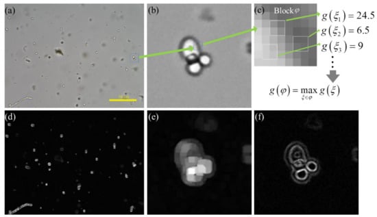
Figure 2.
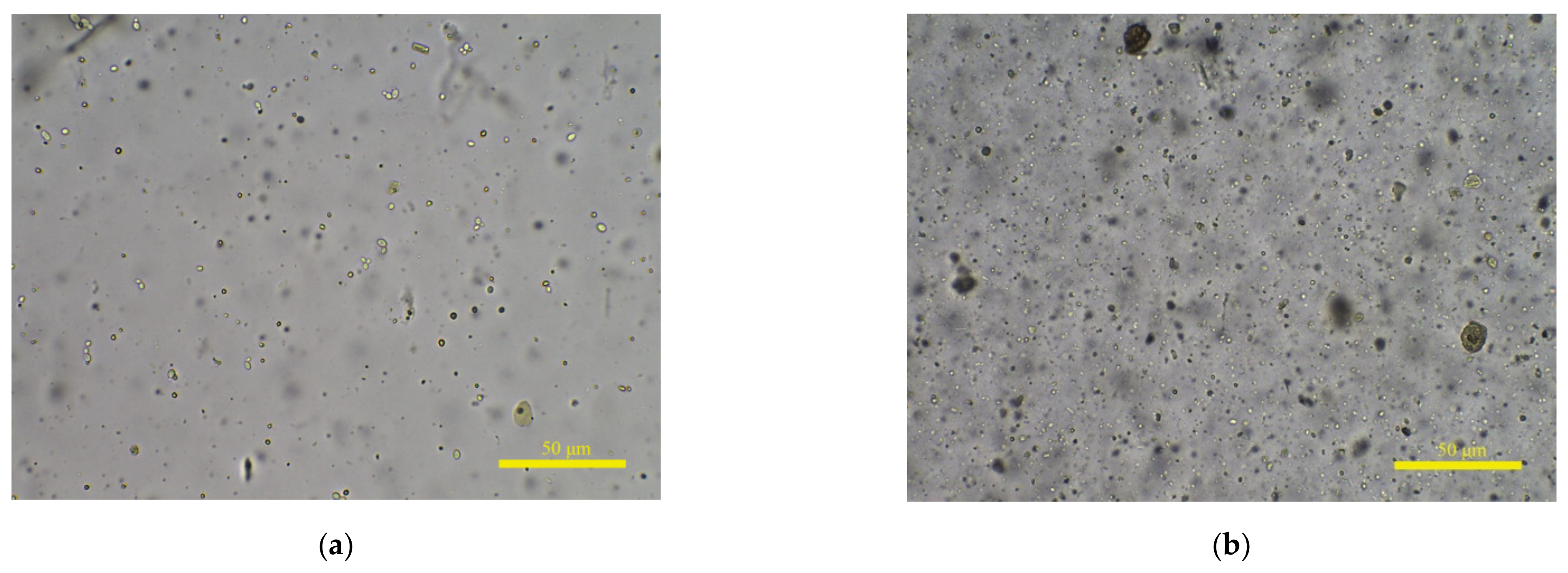
The calculation process of local maximum gradient method. (a) is a fecal microscopic image with fungal spores. (b) is a local enlargement image of a fungal spore in (a). (c) is a 8 × 8 image patch, which is defined as block . (d,e) is the feature image of (a,b) calculated by local maximum gradient method with and equal to 1. (f) is the feature map of (b) calculated by Tenengrad method. (d–f) are visual images after normalizing image pixel value to 0–255.
Finally, the image is divided into overlapping with stride of and in the horizontal and vertical directions. By calculating of each Block , the feature map of the local maximum gradient is obtained. Shown in Figure 2a is a fecal microscopic image with fungal spores, and (b) is a local enlargement image of a fungal spore in (a). The local maximum gradient image of (a) and (b) is shown in (d) and (e), respectively. (f) is the gradient map of (b) calculated by the Tenengrad method [7]. The internal region of a sharp fungal spore is a flat area with high brightness, and it has a high gradient value in the local maximum gradient image. However, its gradient value is low in the Tenengrad gradient image and is close to the background response. Comparing (e) and (f), the Tenengrad method focuses on sharp edges but the local maximum gradient method focuses on sharp objects. Using Figure 2e as the gradient attention mechanism can force the CNN to focus on clear objects.
In the Supplementary Materials, we demonstrate the prediction accuracy of the local maximum gradient method used as a gradient-based IQA method on finding the clearest human fecal microscopic image in the autofocus process.
3.2. Network Architecture
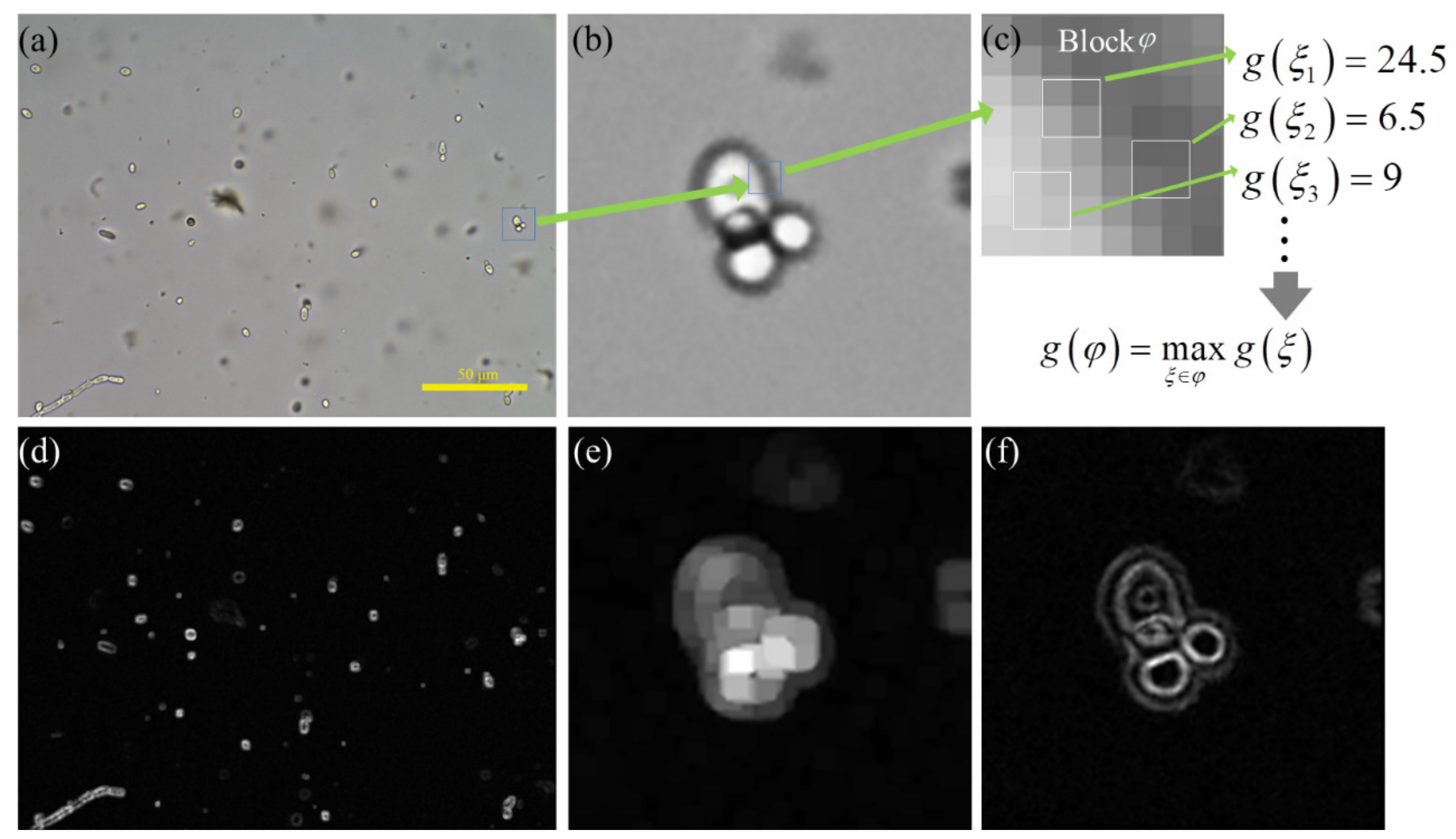
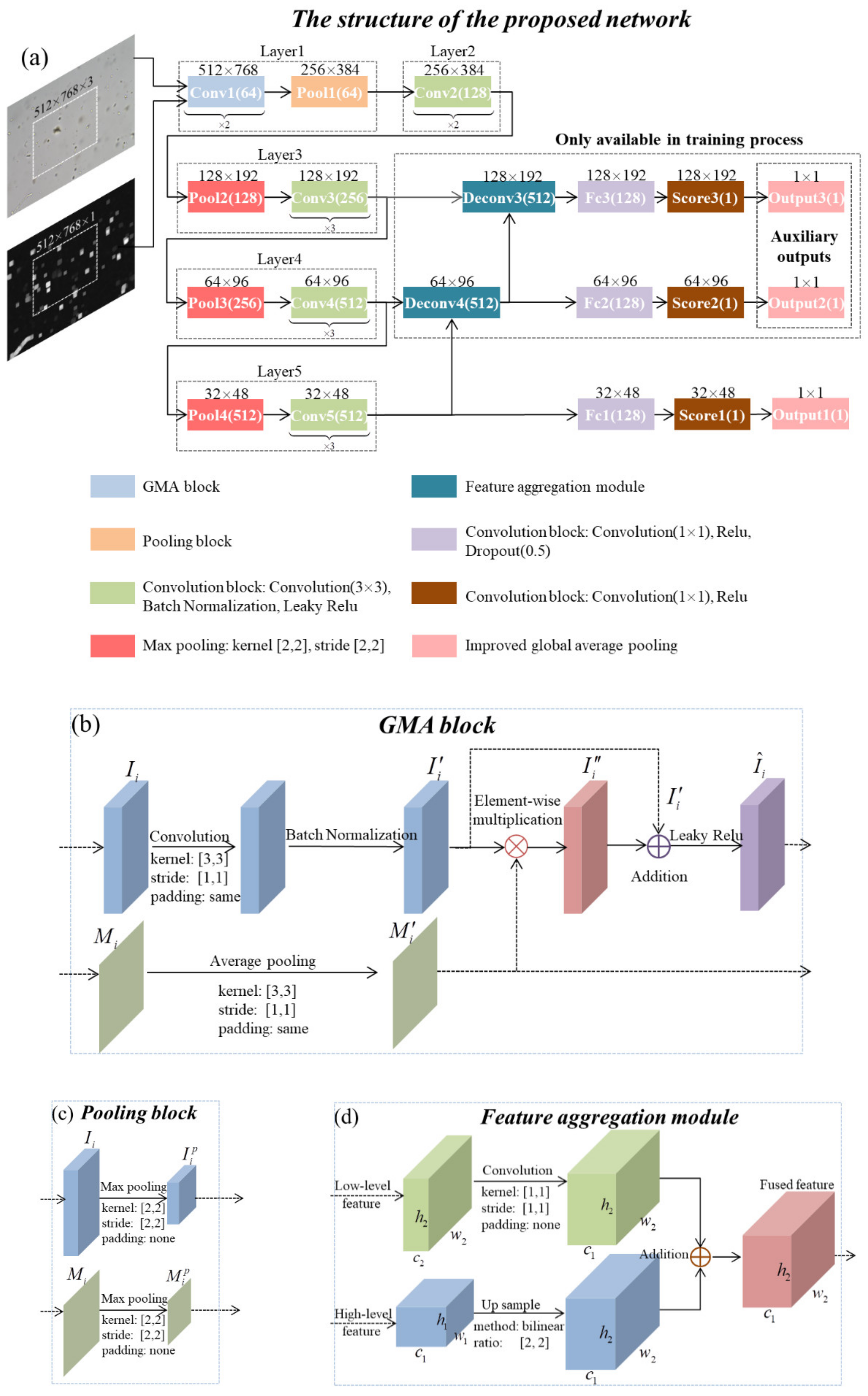
The structure of the proposed GMANet is shown in Figure 3a and the framework is based on the VGG16 [27] architecture. Through comparative experiments, we found that the performance of VGG16 is similar to that of other backbones, such as resnet50. Considering the simplification of the model, VGG16 was used as the backbone. The gradient image extracted by the local maximum gradient method was introduced into the CNN as an attention map, and Figure 3b shows the specific structure of the convolution block with MA, namely the GMA block.
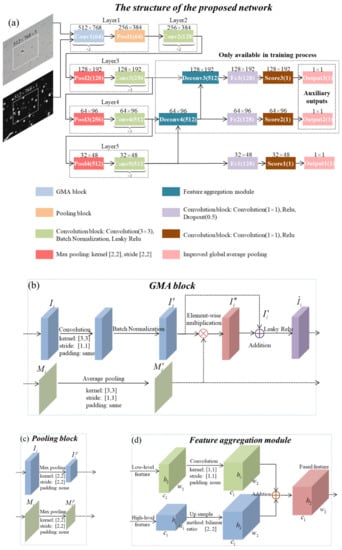
Figure 3.
(a) The structure of the proposed GMANet. (b) The structure of the GMA block. (c) The structure of the pooling block. (d) The structure of the feature aggregation module.
The input of the GMA block is a 3-D input feature map and its corresponding 2-D spatial attention map , where i represents the i-th convolution block. Firstly, the operation of convolution and batch normalization is performed on input to obtain ; secondly, the operation of average pooling (the pooling parameter is same as the convolution on ) is performed on input to obtain ; thirdly, the features of are adjusted by attention map through element-wise multiplication, obtaining adjusted feature map . Finally, and are added together and the operation of Leaky Relu is performed on the addition result, obtaining feature map . and are the input of the next GMA block. The MA mechanism does not change the network structure or increase the training parameters, but it enhances the feature values in high-gradient regions. The calculation process can be summarized as:
The specific structure of the pooling block is shown in Figure 3c. When the feature matrix performs the max pooling operation, the corresponding spatial attention map performs the same operation. The feature aggregation module is shown in Figure 3d. Two low-level feature maps named Deconv3 and Deconv4 are obtained by feature aggregation, and the size of them are 128 × 192 × 512 and 64 × 96 × 512.
Most deep-learning-based IQA methods use a small patch as network input, and connect fully connected layers at the end of the feature extraction layer to predict the score of the current patch. These patch-based IQA methods only consider the local information while ignoring the global information. Furthermore, the local quality of a small image patch is not equal to the real score of the whole image. In order to solve the above problem, a large image patch with a fixed size of 512 × 768 × 3 was used. At the end of the feature extraction layer (Layer5, size: 32 × 48 × 512), every feature vector with a size of 1 × 1 × 512 is regarded as an independent patch sample feature. After connecting them with two convolutional layers, the predicted score map is obtained with a size of 32 × 48 × 1. The final prediction score, Output1, is calculated by the improved global average pooling, which computes the average of non-zero values in the predicted score map. To speed up training and reduce over-fitting, we used low-level feature maps Deconv3 and Deconv4 to generate auxiliary outputs (Output2 and Output3). The loss weights of Output1 to Output3 were 1.0, 0.8, and 0.6. Output2 and Output3 were used to assist network training, and only Output1 was calculated in the inference phase.
In order to eliminate the influence of image brightness and contrast, the gray microscopic image is normalized by z-score normalization before calculating the gradient. We only introduced MA in Layer1, and the ablation experiments of introducing MA into Layer2 are discussed in Section 4. In the Supplementary Materials, we analyze the interference effect of blurred regions on finding the clearest fecal microscopic images by traditional IQA methods, which proves the effectiveness of the gradient mask attention mechanism in this regard.
3.3. Loss
The loss function that we used includes two types of losses:
where is the total loss of one iteration; is the score loss between the predicted score and annotated score; is the rank loss between the clearest image and distorted images. is a Boolean value to control .
The score loss makes the predicted score closer to the annotated score, which is defined as:
where M is the batch size used in the training process; is the smooth loss; is the predicted score, and s is the annotated score.
The Rank-IQA [21] method has proven that the ranking information between distorted images is useful to make a CNN model more consistent with HVS. We decided to use an improved rank loss [28] and it is defined as:
where and represent the predicted and annotated score of the clearest image in one group of microscopic images; and represent the predicted and annotated score of the distorted image in the same group of microscopic images. The improved rank loss contains the information of score loss. When the rank order is correct in one iteration (), score loss is calculated twice, which is not conducive to model training. Therefore, we used a Boolean value to control the total loss , and it is defined as:
3.4. Training and Inference
The specific parameters and settings during training were as follows: batch size was 7 and Adam [29] was selected as the optimizer. Learning rate was set to 10−5 and decay rate was 5 × 10⁻⁵. When the training process reached the 32nd epoch, the learning rate decayed to approximately 1/2 of the original. We set to 32 × 32 to calculate the local maximum gradient. The size of formed elements such as fungal spores, red blood cells, and white blood cells in fecal microscopic images is approximately 30 × 30 to 90 × 90. Taking the maximum gradient in a 32 × 32 region as the response value can ensure that the region of a clear object in the gradient map has a high gradient value. The size of fecal microscopic images was rescaled to 1024 × 1536 with bilinear interpolation (the origin image size was 1200 × 1600). The color and gray image were normalized by z-score normalization, and then the gradient image of the local maximum gradient was computed. Regions of a fixed size of 512 × 768 were randomly cropped in the color and gradient image. This large image patch can ensure that the GMANet fully learns the global information of the image. In addition, when the patch is large enough, we can assume that its annotated score is equal to that of the whole image. We divided the training process into two stages. Firstly, we trained the network without MA for 70 epochs, and the optimal model L0 with minimum on the validation set was selected. Then, the MA was introduced into Layer1. L0 was used as a pre-trained model for transfer learning. After training 40 epochs, the optimal model L1 with minimum on the validation set was the final score model. For model L0, the backbone VGG16 of GMANet used the pre-training parameters trained on ImageNet and other network parameters were initialized by the Xavier method. For model L1, all the network parameters were initialized by the optimal model L0.
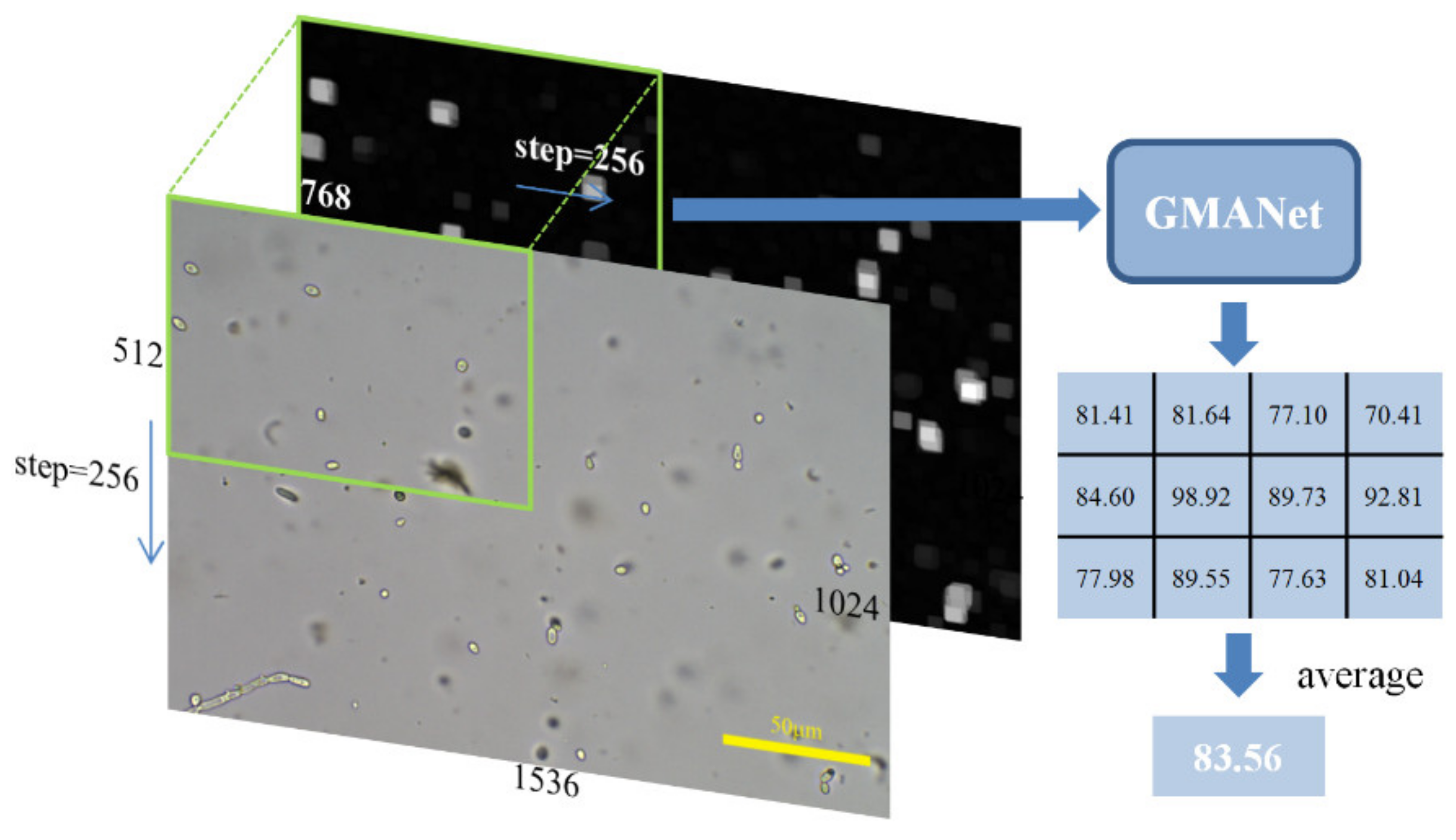
The inference process is shown in Figure 4. By scaling and normalization the same as introduced in the training process, the color image with a size of 1024 × 1536 × 3 and the gradient image with a size of 1024 × 1536 × 1 could be obtained. A patch of fixed size of 512 × 768 was cropped in the color and gradient image with a step of 256 in the horizontal and vertical direction. The cropping step enables the object at the patch boundary to be located around the central area in the next patch, ensuring that GMANet can evaluate all objects in the image. The predicted quality of the whole image can be obtained by calculating the average of the predicted scores of all large patches.

Figure 4.
The inference process of proposed network.
4. Experimental Results and Dataset
4.1. Dataset
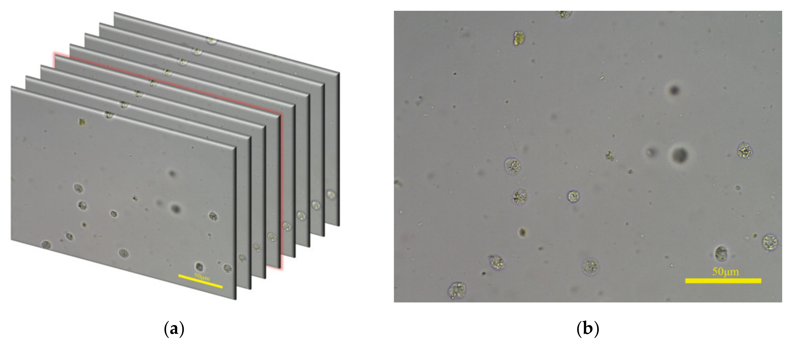
The feces dataset used in this paper contains 1036 groups of fecal microscopic images, with a total of 15,645 images. Each image group is captured in the autofocus process. For each field of view, the microscope platform is continuously moved along the z-axis and a microscope camera takes pictures simultaneously. The start position of microscope platform in the z-axis is the defocusing position and the end position is the defocusing position at the other end; thus, the image composition changes from blurred to clear and then to blurred. For example, one group of images is shown in Figure 5a. The image with red highlights on the edges is the clearest image in this group and it is shown in Figure 5b.
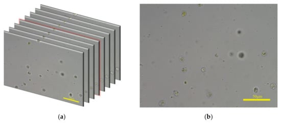
Figure 5.
(a) One group of fecal microscopic images captured in autofocus process; some images are omitted for ease of interpretation. (b) The clearest image of the image group in (a).
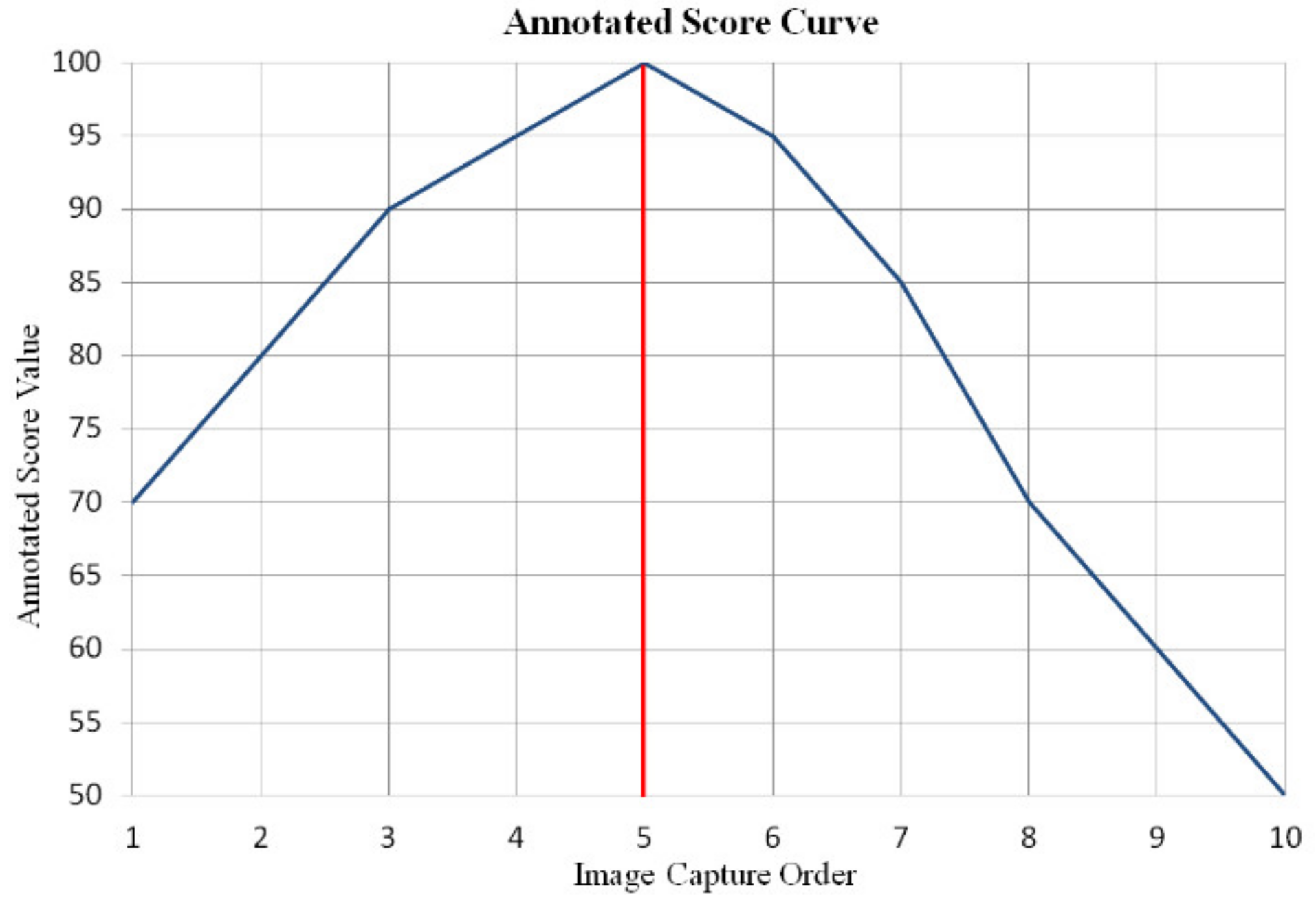
We annotated the feces dataset with the help of specialists in laboratory medicine, and each image was marked with a score based on human perception. Comparing the clarity between two images captured from different autofocus processes is difficult; thus, the annotated score was a relative value in each image group. The specific scoring rules in each image group were as follows: (1) the score of clearest image was 100, and remaining clear images were assigned from 95 to 99; (2) with regard to blurred images, the scores were assigned from 94 to 0 according to the degree of blur relative to the clearest image. Figure 6 shows the annotated score curve of the image group in Figure 5a. The image size of the fecal microscopic image is 1200 × 1600 × 3.
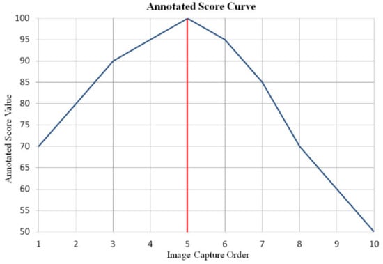
Figure 6.
Annotated score curve of the image group displayed in Figure 5a. The abscissa is the image capture order in the autofocus process, and the 5th image is the clearest image. The ordinate is the annotated score value.
For the training phase, we randomly divided the feces dataset into a training, validation, and test set according to the ratio of 0.6:0.2:0.2. Because of the use of rank loss, the dataset was divided according to image groups instead of randomly shuffling all images, obtaining 621 image groups in the training set, 207 image groups in the validation set, and 208 image groups in the test set. In each iteration, one image group was selected from the training set, and then the clearest image was picked and batch-1 images were randomly chosen.
In order to assess the generality of the proposed method, GMANet trained on the feces dataset was verified on additional leucorrhea and blood datasets without transfer learning. The process of image acquisition of these two datasets was the same as that of the feces dataset. The leucorrhea dataset contained 699 groups of leucorrhea microscopic images, with a total of 23,319 images. The blood dataset contained 130 groups of blood microscopic images, with a total of 6116 images. Due to the heavy workload of scoring each image in the two datasets, we only annotated the image capture order of the clearest image in each group. The image sizes of the leucorrhea and blood microscopic images were 1200 × 1920 × 3 and 1200 × 1600 × 3, respectively.
We used a Motic B1Digital microscope with a 40× objective lens (Numerical Aperture (NA): 0.65, Material Distance: 0.6 mm) to capture fecal and blood microscopic images. The leucorrhea microscopic images were captured by a Motic CX31 biological microscope with a 40× objective lens (NA: 0.65, Material Distance: 0.6 mm) and a Motic EXCCD01400KMA CCD camera. The study was conducted according to the guidelines of the Declaration of Helsinki, and approved by the Institutional Review Board of the University of Electronic Science and Technology of China (protocol code: 106142021030903).
4.2. Performance Metric
In order to evaluate the performance of the IQA methods, two performance metrics were adopted: SROCC and prediction accuracy.
4.2.1. Spearman Rank-Order Correlation Coefficient
SROCC is a commonly used metric that has the ability to measure the correlation between predicted scores and annotated scores. A value close to 1 indicates high performance of the IQA method. It can be computed as follows:
where is the difference between the i-th image ranks in annotated scores and predicted scores; n is the number of images in the evaluation dataset. As the annotated score was a relative value in each group of images, we calculated the SROCC value of each evaluation image group and finally calculated the average value of them.
4.2.2. Prediction Accuracy
The goal of our research was to identify the clearest image in a group of images, so the accuracy of judging the clearest image was an important evaluation indicator. In each image group, we defined the capture order of each image in the autofocus process as , where n is the number of images in this group. Furthermore, we defined the capture order of the image with the maximum predicted score as , and the capture order of the image with the maximum annotated score as . When is equal to , the prediction of the IQA method is consistent with HVS in this image group, and we defined the corresponding group as type “top-0”. When is not equal to but the absolute difference between them is 1, the prediction of the IQA method is slightly different from HVS, and we defined the corresponding image group as type “top-1”. In [3], we proposed a super depth of field (SDoF) network to detect cells by an SDoF feature aggregation module. The inputs of SDoF-Net are three microscopic images (the clearest image and its preceding and succeeding image), which are captured in one autofocus process. Therefore, image groups with type “top-0” and “top-1” are acceptable for our research. We defined and to represent the number of image groups with type “top-0” and “top-1”, respectively. Furthermore, we defined “acc” to represent the proportion of the sum of and in the number of evaluation image groups.
4.3. Experimental Results
In order to eliminate the performance bias of the proposed method, we repeated the whole training process five times, and the corresponding results on the test set, leucorrhea dataset, and blood dataset are shown in Table 1. “srocc” represents the average SROCC value in the evaluation image group. The selection of optimal models on the validation set is described in Section 3.4. To prevent under-fitting or over-fitting, the L0 model should also meet the following conditions: “acc” should be higher than 98% and lower than 99%; should be between 120 and 129. The L1 model only needs to meet the requirement that “acc” is higher than 98%. Blood and leucorrhea microscopic images were rescaled to the size of 1024 × 1536 and 768 × 1152. The same normalization method was adopted and the patch cropping step was 256 and 384 in the horizontal and vertical direction for them. The size of was set to 32 × 32 for the blood microscopic image and 8 × 8 for the leucorrhea microscopic image. We used the tensorflow2 framework to build our algorithm and ran it on a RTX 3090 GPU.

Table 1.
The model performance on test set, leucorrhea dataset, and blood dataset.
It can be seen from Table 1 that: L0 can easily over-fit on the validation set, and its prediction accuracy on the test set is unstable; the L0 in Round 5 over-fits on the feces dataset and cannot be used for the leucorrhea dataset; L1 achieves good prediction accuracy on the feces dataset and it is more consistent with HVS ( on test set is higher); L1 can improve the prediction accuracy on the leucorrhea dataset better than L0, especially the L0 in Round 5; for the blood dataset with simple compositions, both L0 and L1 can achieve excellent results.
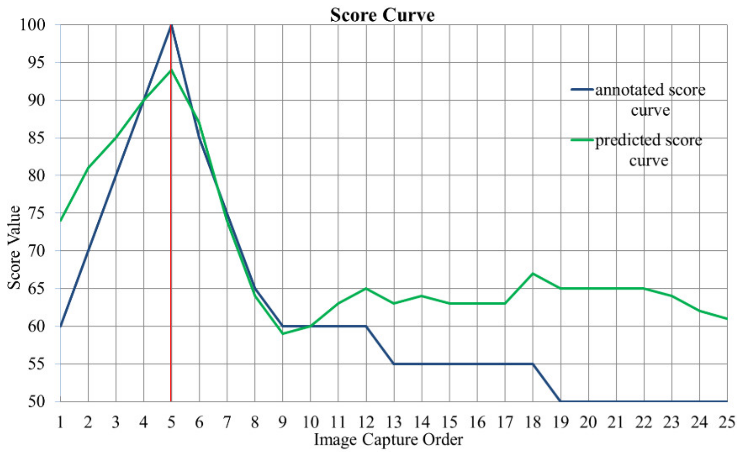
In the training process, we also tried to use the model with the largest average SROCC value as the optimal model, but the model prediction accuracy was unstable. As shown in Figure 7, for one fecal microscopic image group in the test set, the blue and green curve represent the predicted score curve calculated by model L1 (Round 3) and the annotated score curve, respectively. Although the image capture order is equal to in this image group, the predictions of blurred image scores are inaccurate, leading to a low SROCC value, which is 0.5016. Considering that our goal was to find the clearest image, we only regarded the SROCC value as a reference, not as an evaluation metric for model selection.
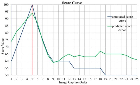
Figure 7.
Score curve of one fecal microscopic image group in test set. The abscissa is the image capture order in the autofocus process, and the 5th image is the clearest image. The ordinate is the score value. The blue and green curve represent annotated and predicted score curve, respectively. The SROCC value of this image group is 0.5016.
Some formed elements in leucorrhea are similar to those in feces, such as white blood cells, fungal spores, and red blood cells, and the cell morphology is comparable. Similarly, blood samples also contain red blood cells and white blood cells. Although the models were trained on the feces dataset, some L0 could achieve acceptable results on the leucorrhea and blood datasets, with poor robustness of model performance. To show the availability of MA, we plotted the attention heat maps visualized by Grad-CAM++ [30]. Figure 8 presents the attentions in the output of Layer5 of L0 and L1. It can be seen that the attentions of model L0 are mainly distributed around the regions of fungal spores and impurities. After applying MA, the attentions in blurred regions or the background are suppressed. This indicates that the introduction of MA causes the network to pay more attention to sharp regions.

Figure 8.
The attention heat maps of fecal microscopic image visualized by Grad-CAM++. (a,b) presents the attentions in the output of Layer5 of L0 and L1, respectively.
The performance of GMANet based on backbone resnet50 is shown in the Supplementary Materials.
5. Discussion
5.1. Ablation Study
5.1.1. The Influence of Introduction Depth of MA
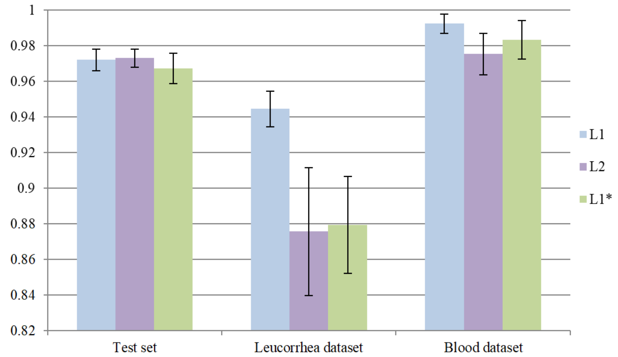
In this part of the experiment, we introduced MA into Layer2 to verify whether the model performance could be promoted. Similarly, L1 was used as a pre-trained model for transfer learning. After training 40 epochs, the optimal model with minimum on the validation set was defined as L2. In addition, we further verified the effect of two-stage training. We directly trained the network with MA into Layer1 and the optimal model with minimum on the validation set was defined as . L2 and need to meet the requirement that “acc” is higher than 98%. Similarly, we repeated the whole training process five times for model L2 and . The comparisons between L1, and L2 are shown in Figure 9. To simplify the process of comparing, we only demonstrated the average “acc” of three models. It can be seen that further introducing MA into Layer2 can slightly improve the performance on the test set but greatly reduces the performance on the leucorrhea dataset. Both L2 and over-fit on the feces dataset. As a result, directly training the network with MA is less effective than two-stage training.
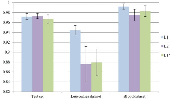
Figure 9.
The effectiveness of introducing MA into the network with different depths.
5.1.2. The Influence of Using Different Gradient Methods to Compute Attention Map
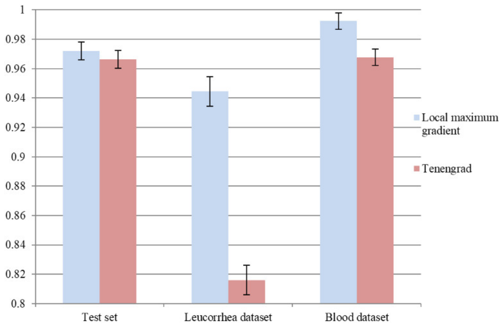
To verify the effectiveness of the local maximum gradient method, we adopted the frequently used Tenengrad [7] method to compute a gradient image as an attention map. We retrained L1 based on the L0 in Section 4.3, and the same training process and optimal model selection criterion were used. The comparison of average “acc” on the test set, leucorrhea dataset, and blood dataset is shown in Figure 10. It can be seen that using Tenengrad to compute the attention map could lead to over-fitting on the feces dataset. The local maximum gradient method, which concentrates on local regions rather than edges, is more suitable for microscopic image quality evaluation.

Figure 10.
The influence on model performance of using Tenengrad method to compute attention map.
5.1.3. The Effectiveness of Using Auxiliary Outputs in Training Process
To prove the availability of using auxiliary outputs in the training process, we only used Output1 to compute the loss and train the network for another five rounds. The network without MA was trained for 100 epochs, and other settings and parameters were unchanged. The corresponding results on the test set, leucorrhea dataset, and blood dataset are shown in Table 2.
Table 2.
The performance of model trained without auxiliary outputs.
It can be seen that in the absence of auxiliary outputs, the average “acc” of L0 on the test set is increased but it easily over-fits on the feces dataset, resulting in poor performance on the leucorrhea dataset. The over-fitting can even lead to a performance degradation in L1, such as the model in Round 5. The performance of L1 in Round 1 to Round 4 further proves the effectiveness of the gradient MA mechanism.
5.2. Comparison with Deep-Learning-Based IQA Methods
In this part of the experiment, we compared the proposed model with two deep-learning-based methods: TwostreamIQA [15] and WaDIQaM-FR [31]. TwostreamIQA uses the gradient image as the features to be learned. WaDIQaM-FR adds a patch weight estimate module at the end of the feature extraction layers, and the predicted score of each image is the weighted sum of all patch scores. WaDIQaM-FR is a kind of FR-IQA method that needs a reference image. We used the assumption in [32]—that is, the clearer the image is, the greater the difference between its Gaussian blurred image and the original image is. A Gaussian blur operation with a kernel size of 21 and sigma value of 3.5 was performed on all datasets, and then the original images and corresponding Gaussian blurred images were used as reference images and distorted images, respectively. We repeated the training process five times and adopted a similar optimal model selection method. The comparison of average “acc” on the test set, leucorrhea dataset, and blood dataset is shown in Figure 11. We also tested the WaDIQaM-NR [31] method, but its prediction accuracy on the validation set was lower than 97%.
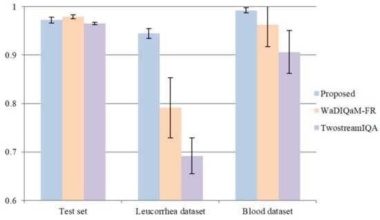
Figure 11.
Comparison with two deep-learning-based NR-IQA methods.
From the results, we can see that the proposed model outperformed the other two deep-learning-based IQA methods. Both the TwostreamIQA and WaDIQaM-FR methods achieved excellent prediction accuracy on the feces dataset, and their average “acc” on the test set was 96.539% and 97.885%, respectively. However, they could not achieve valid results on the leucorrhea dataset. Although we normalized the gradient images in advance so that the gradient features of different images were at the same magnitude, the gradient distribution of images in different datasets was still different. Therefore, the deep model trained on the feces dataset by the TwostreamIQA method was only applicable for the feces dataset. The patch score and weight in WaDIQaM-FR are trainable parameters, which were trained on the feces dataset. As a result, the predicted score and weight in the feces dataset were exact but they were inaccurate in the leucorrhea dataset.
In order to further prove the effectiveness of GMANet, in the Supplementary Materials, we demonstrate the performance of 37 types of traditional IQA methods on finding the clearest human fecal microscopic image in the autofocus process. Furthermore, we analyze the reasons for the poor performance of traditional IQA methods.
5.3. Limitations and Future Work
5.3.1. Limitation on Real-Time Detection
The average calculation time of quality assessment for one fecal microscopic image is shown in Table 3. A fecal microscopic image can be divided into 12 image patches with a fixed size of 512 × 768. These patches can be concatenated along the batch channel and be detected in one single inference. The total average calculation time reaches 248 ms per image. In general, an image group captured in the autofocus process contains 10 to 30 images; that is, it takes 2 to 7 s to find the clearest image. Therefore, the proposed model still has a limitation regarding real-time detection.
Table 3.
The average calculation time of predicting the quality of one fecal microscopic image.
5.3.2. Limitation on Applying to Leucorrhea Dataset
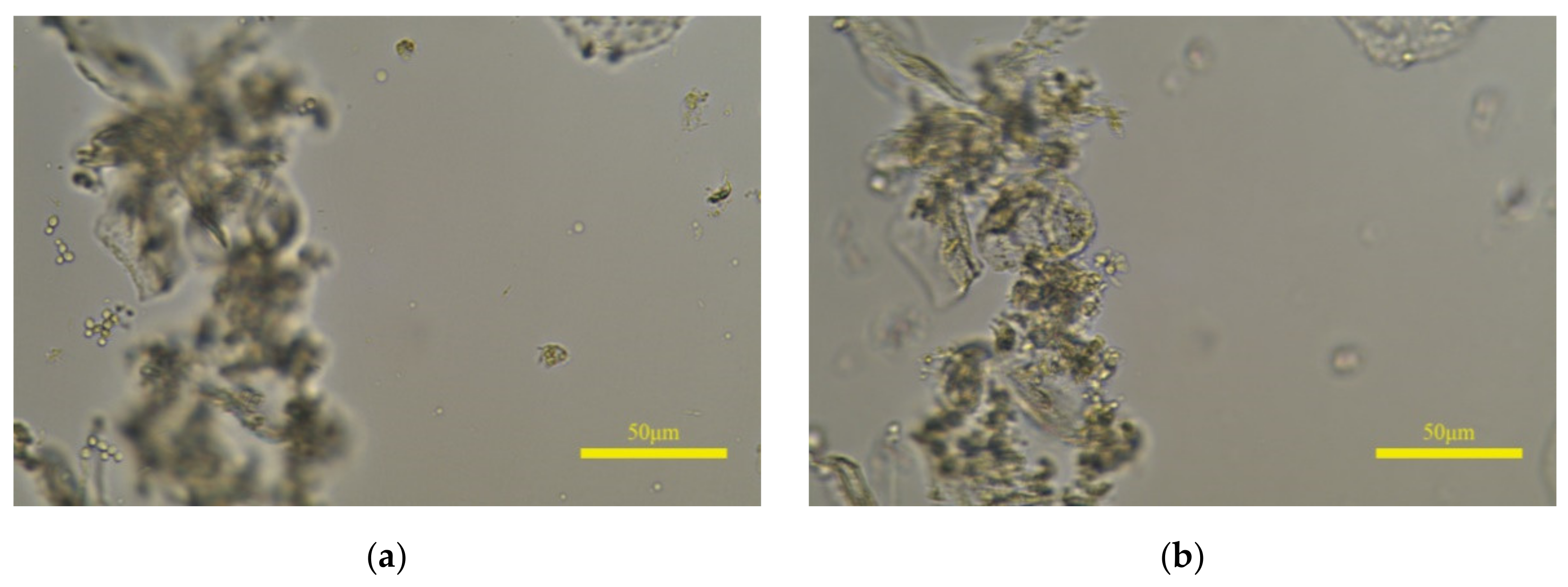
There are still differences between the prediction of the proposed model and the perception of HVS. If leucorrhea microscopic images contain epithelial cells with a large size, the model will predict the clear image of epithelial cells as the clearest. Shown in Figure 12a is the annotated clearest image in one image group, and (b) is the predicted clearest image. The white blood cells and fungal spores in (a) are clear, and the epithelial cells are defocused but still can be recognized; the situation in (b) is the opposite and the white blood cells or fungal spores cannot be identified. If (b) is input into the object detection algorithm, the qualitative judgment result may be inaccurate. Furthermore, the rescaled size of 768 × 1152 and the 8 × 8 size of are the optimal parameters selected after multiple tests. As the sizes of and the image increase, the “acc” value on the leucorrhea dataset gradually decreases. When the image size is 1024 × 1536 and the size of is 32 × 32, the “acc” value drops below 70%.
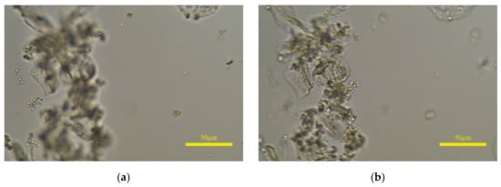
Figure 12.
The influence of epithelial cells with large size on prediction results. (a,b) are the annotated and predicted clearest image in one image group, respectively.
5.3.3. Future Work
The above limitations restrict the efficiency and generality of our proposed GMANet. In future work, we will simplify the network structure to accelerate the computing speed and improve the generality of the deep model. Furthermore, we will verify whether other shallow features, such as edge, phase, and contrast, used in traditional NR-IQA methods, can be introduced as an MA map.
In our previous work, we fused clear image patches in different locations and the corresponding experimental results are described in [33]. In order to verify the performance of GMANet on assessing the clarity of objects, we used the image fusion method to stitch the clearest image patches together. Details are described in the Supplementary Materials. Using a deep learning method to fuse the microscopic images captured in the autofocus process into one clear microscopic image is our next research direction.
6. Conclusions
In this paper, we proposed a blind IQA method based on a deep CNN to solve the difficulty of finding the clearest image in a microscopic image group captured in the autofocus process, namely GMANet. We introduced the gradient information into a low-level convolution block as spatial attention to make the high-level features pay more attention to sharp regions. Experimental results show that the proposed network has good consistency with human visual properties. As gradient images are not features to be learned, the deep model trained on the feces dataset is universal, and can be applied to leucorrhea and blood microscopic image quality assessment without additional transfer learning. Our study has value for addressing the autofocus task for microscopic images with complex composition.
Supplementary Materials
The following are available online at https://www.mdpi.com/article/10.3390/app112110293/s1, Experiment 1: Using traditional IQA methods to find clearest fecal microscopic image, Experiment 2: Using resnet50 as GMANet backbone, Experiment 3: The performance of GMANet on assessing the clarity of objects.
Author Contributions
Project administration, L.L.; investigation, G.N.; resources, G.N.; data curation, X.W.; methodology, X.W.; writing—original draft preparation, X.W.; writing—review and editing, X.D.; funding acquisition, J.Z. and J.L. All authors have read and agreed to the published version of the manuscript.
Funding
This research was funded by the National Natural Science Foundation of China (No. 61905036), the Fundamental Research Funds for the Central Universities (University of Electronic Science and Technology of China) (No. ZYGX2019J053), and the China Postdoctoral Science Foundation (2019M663465).
Institutional Review Board Statement
The study was conducted according to the guidelines of the Declaration of Helsinki and approved by the Institutional Review Board of the University of Electronic Science and Technology of China (protocol code: 106142021030903).
Informed Consent Statement
Written informed consent was obtained from the patients to publish this paper. All samples were anonymized.
Data Availability Statement
The algorithm codes will be released online at www.github.com/wxz92/GMANet, accessed on 1 November 2021.
Acknowledgments
We would like to express our thanks to Yu-Tang Ye and the staff at the MOEMIL laboratory, who collected and counted the samples used in this study.
Conflicts of Interest
The authors declare no conflict of interest.
References
- Khouani, A.; El Habib Daho, M.; Mahmoudi, S.A.; Chikh, M.A.; Benzineb, B. Automated recognition of white blood cells using deep learning. Biomed. Eng. Lett. 2020, 10, 359–367. [Google Scholar] [CrossRef]
- Du, X.H.; Liu, L.; Wang, X.Z.; Ni, G.M.; Zhang, J.; Hao, R.Q.; Liu, J.X.; Liu, Y. Automatic classification of cells in microscopic fecal images using convolutional neural networks. Biosci. Rep. 2019, 39, BSR20182100. [Google Scholar] [CrossRef] [PubMed] [Green Version]
- Du, X.; Wang, X.; Ni, G.; Zhang, J.; Hao, R.; Zhao, J.; Wang, X.; Liu, J.; Liu, L. SDoF-Net: Super Depth of Field Network for Cell Detection in Leucorrhea Micrograph. IEEE J. Biomed. Health Inform. 2021. [Google Scholar] [CrossRef]
- Wang, Z.; Bovik, A.C.; Sheikh, H.R.; Simoncelli, E.P. Image quality assessment: From error visibility to structural similarity. IEEE Trans. Image Process. 2004, 13, 600–612. [Google Scholar] [CrossRef] [Green Version]
- Zhang, L.; Zhang, L.; Mou, X.Q.; Zhang, D. FSIM: A Feature Similarity Index for Image Quality Assessment. IEEE Trans. Image Process. 2011, 20, 2378–2386. [Google Scholar] [CrossRef] [PubMed] [Green Version]
- Sheikh, H.R.; Bovik, A.C. Image information and visual quality. IEEE Trans. Image Process. 2006, 15, 430–444. [Google Scholar] [CrossRef]
- Yeo, T.T.E.; Ong, S.H.; Jayasooriah; Sinniah, R. Autofocusing for Tissue Microscopy. Image Vis. Comput. 1993, 11, 629–639. [Google Scholar] [CrossRef]
- Kristan, M.; Pers, J.; Perse, M.; Kovacic, S. A Bayes-spectral-entropy-based measure of camera focus using a discrete cosine transform. Pattern Recognit. Lett. 2006, 27, 1431–1439. [Google Scholar] [CrossRef] [Green Version]
- Narvekar, N.D.; Karam, L.J. A No-Reference Image Blur Metric Based on the Cumulative Probability of Blur Detection (CPBD). IEEE Trans. Image Process. 2011, 20, 2678–2683. [Google Scholar] [CrossRef]
- Blanchet, G.; Moisan, L. An explicit sharpness index related to global phase coherence. In Proceedings of the 2012 IEEE International Conference on Acoustics, Speech, and Signal Processing, ICASSP 2012, Kyoto, Japan, 25–30 March 2012; pp. 1065–1068. [Google Scholar]
- Oszust, M. No-reference image quality assessment with local features and high-order derivatives. J. Vis. Commun. Image Represent. 2018, 56, 15–26. [Google Scholar] [CrossRef]
- Kang, L.; Ye, P.; Li, Y.; Doermann, D.; IEEE. Convolutional Neural Networks for No-Reference Image Quality Assessment. In Proceedings of the 27th IEEE Conference on Computer Vision and Pattern Recognition (CVPR), Columbus, OH, USA, 23–28 June 2014; pp. 1733–1740. [Google Scholar]
- Sheikh, H.R.; Sabir, M.F.; Bovik, A.C. A statistical evaluation of recent full reference image quality assessment algorithms. IEEE Trans. Image Process. 2006, 15, 3440–3451. [Google Scholar] [CrossRef]
- Ponomarenko, N.; Jin, L.; Ieremeiev, O.; Lukin, V.; Egiazarian, K.; Astola, J.; Vozel, B.; Chehdi, K.; Carli, M.; Battisti, F.; et al. Image database TID2013: Peculiarities, results and perspectives. Signal Process. Image Commun. 2015, 30, 57–77. [Google Scholar] [CrossRef] [Green Version]
- Yan, Q.S.; Gong, D.; Zhang, Y.N. Two-Stream Convolutional Networks for Blind Image Quality Assessment. IEEE Trans. Image Process. 2019, 28, 2200–2211. [Google Scholar] [CrossRef]
- Yang, S.; Jiang, Q.P.; Lin, W.S.; Wang, Y.T. SGDNet: An End-to-End Saliency-Guided Deep Neural Network for No-Reference Image Quality Assessment. In Proceedings of the 27th ACM International Conference on Multimedia (MM), Nice, France, 21–25 October 2019; pp. 1383–1391. [Google Scholar]
- Po, L.M.; Liu, M.Y.; Yuen, W.Y.F.; Li, Y.M.; Xu, X.Y.; Zhou, C.; Wong, P.H.W.; Lau, K.W.; Luk, H.T. A Novel Patch Variance Biased Convolutional Neural Network for No-Reference Image Quality Assessment. IEEE Trans. Circuits Syst. Video Technol. 2019, 29, 1223–1229. [Google Scholar] [CrossRef]
- Chetouani, A.; Li, L.D. On the use of a scanpath predictor and convolutional neural network for blind image quality assessment. Signal Process. Image Commun. 2020, 89, 115963. [Google Scholar] [CrossRef]
- Ren, H.Y.; Chen, D.Q.; Wang, Y.Z. RAN4IQA: Restorative Adversarial Nets for No-Reference Image Quality Assessment. In Proceedings of the 32nd AAAI Conference on Artificial Intelligence/30th Innovative Applications of Artificial Intelligence Conference/8th AAAI Symposium on Educational Advances in Artificial Intelligence, New Orleans, LA, USA, 2–7 February 2018; pp. 7308–7314. [Google Scholar]
- Hu, J.B.; Wang, X.J.; Shao, F.; Jiang, Q.P. TSPR: Deep network-based blind image quality assessment using two-side pseudo reference images. Digit. Signal Process. 2020, 106, 102849. [Google Scholar] [CrossRef]
- Liu, X.L.; de Weijer, J.V.; Bagdanov, A.D.; IEEE. RankIQA: Learning from Rankings for No-reference Image Quality Assessment. In Proceedings of the 16th IEEE International Conference on Computer Vision (ICCV), Venice, Italy, 22–29 October 2017; pp. 1040–1049. [Google Scholar]
- Ma, K.D.; Duanmu, Z.F.; Wu, Q.B.; Wang, Z.; Yong, H.W.; Li, H.L.; Zhang, L. Waterloo Exploration Database: New Challenges for Image Quality Assessment Models. IEEE Trans. Image Process. 2017, 26, 1004–1016. [Google Scholar] [CrossRef]
- Zhou, B.L.; Lapedriza, A.; Xiao, J.X.; Totralba, A.; Oliva, A. Learning Deep Features for Scene Recognition using Places Database. In Proceedings of the 28th Conference on Neural Information Processing Systems (NIPS), Montreal, QC, Canada, 8–13 December 2014. [Google Scholar]
- Guan, X.D.; He, L.J.; Li, M.Y.; Li, F. Entropy Based Data Expansion Method for Blind Image Quality Assessment. Entropy 2020, 22, 60. [Google Scholar] [CrossRef] [PubMed] [Green Version]
- Xu, Y.J.; Lam, H.K.; Jia, G.Y. MANet: A two-stage deep learning method for classification of COVID-19 from Chest X-ray images. Neurocomputing 2021, 443, 96–105. [Google Scholar] [CrossRef]
- Vu, C.T.; Phan, T.D.; Chandler, D.M. S-3: A Spectral and Spatial Measure of Local Perceived Sharpness in Natural Images. IEEE Trans. Image Process. 2012, 21, 934–945. [Google Scholar] [CrossRef]
- Simonyan, K.; Zisserman, A. Very Deep Convolutional Networks for Large-Scale Image Recognition. In Proceedings of the 3rd International Conference on Learning Representations (ICLR), San Diego, CA, USA, 7–9 May 2015. [Google Scholar]
- Jiang, X.H.; Shen, L.Q.; Yu, L.W.; Jiang, M.X.; Feng, G.R. No-reference screen content image quality assessment based on multi-region features. Neurocomputing 2020, 386, 30–41. [Google Scholar] [CrossRef]
- Kingma, D.P.; Ba, J.L. Adam: A method for stochastic optimization. In Proceedings of the 3rd International Conference on Learning Representations (ICLR), San Diego, CA, USA, 7–9 May 2015. [Google Scholar]
- Chattopadhay, A.; Sarkar, A.; Howlader, P.; Balasubramanian, V.N.; IEEE. Grad-CAM plus plus: Generalized Gradient-based Visual Explanations for Deep Convolutional Networks. In Proceedings of the 18th IEEE Winter Conference on Applications of Computer Vision (WACV), Tahoe Lake, NV, USA, 12–15 March 2018; pp. 839–847. [Google Scholar]
- Bosse, S.; Maniry, D.; Muller, K.R.; Wiegand, T.; Samek, W. Deep Neural Networks for No-Reference and Full-Reference Image Quality Assessment. IEEE Trans. Image Process. 2018, 27, 206–219. [Google Scholar] [CrossRef] [PubMed] [Green Version]
- Crete, F.; Dolmiere, T.; Ladret, P.; Nicolas, M. The blur effect: Perception and estimation with a new no-reference perceptual blur metric. In Proceedings of the Conference on Human Vision and Electronic Imaging XII, San Jose, CA, USA, 29 January–1 February 2007. [Google Scholar]
- Liu, L.; Du, X.; Liu, J.; Ni, G.; Ren, H. Autofocus System for Imaging Multiple Cells Across Thick Liquid Layers in Differrent Focal Planes. In Proceedings of the 2020 International Conference on Communications, Information System and Computer Engineering (CISCE), Kuala Lumpur, Malaysia, 3–5 July 2020. [Google Scholar]

Publisher’s Note: MDPI stays neutral with regard to jurisdictional claims in published maps and institutional affiliations. |
© 2021 by the authors. Licensee MDPI, Basel, Switzerland. This article is an open access article distributed under the terms and conditions of the Creative Commons Attribution (CC BY) license (https://creativecommons.org/licenses/by/4.0/).