Assignment of Focus Position with Convolutional Neural Networks in Adaptive Lens Based Axial Scanning for Confocal Microscopy

Abstract

Adaptive lenses offer axial scanning without mechanical translation and thus are promising to replace mechanical-movement-based axial scanning in microscopy. The scan is accomplished by sweeping the applied voltage. However, the relation between the applied voltage and the resulting axial focus position is not unambiguous. Adaptive lenses suffer from hysteresis effects, and their behaviour depends on environmental conditions. This is especially a hurdle when complex adaptive lenses are used that offer additional functionalities and are controlled with more degrees of freedom. In such case, a common approach is to iterate the voltage and monitor the adaptive lens. Here, we introduce an alternative approach which provides a single shot estimation of the current axial focus position by a convolutional neural network. We use the experimental data of our custom confocal microscope for training and validation. This leads to fast scanning without photo bleaching of the sample and opens the door to automatized and aberration-free smart microscopy. Applications in different types of laser-scanning microscopes are possible. However, maybe the training procedure of the neural network must be adapted for some use cases.

1. Introduction

Confocal microscopy (CM) is frequently used in life sciences to investigate biological samples, such as tissues and cells, where high spatial resolution is necessary to obtain information about small structures of the sample. The main advantage of CM is the optical sectioning capability, introduced by a confocally aligned pinhole [1,2]. However, CM is a point-wise measurement technique and thus scans in three dimensions are required to acquire three-dimensional information. To accomplish an axial scan, several methods are known. In stage scanning, the sample is moved through the constant focus by a stage as introduced in [3], though motion artefacts in the scan may occur. Another commercially available possibility for axial scanning is a piezo-driven objective holder [4]. Alternatively, deformable mirrors (DM) may also be used for axial scanning [5] and aberration correction [6,7]. In recent years, another general approach based on adaptive lenses (AL) was introduced [2,8,9,10]. By tuning the voltage applied to the AL, the focus shifts axially without the need for any mechanical movement. DMs are easy to control and very powerful, however, they usually have a smaller upstroke compared with AL and require a folded beam, which leads to a bulky optical setup in general. ALs do not need a folded beam because they are translucent elements, so the setup is more compact. There are various realisations of ALs. The most popular concepts include tunable acoustic gradient (TAG) lenses [11], liquid crystal lenses [12], lenses actuated by electrowetting [13], and deformable lenses with piezo actuators [10,14,15].

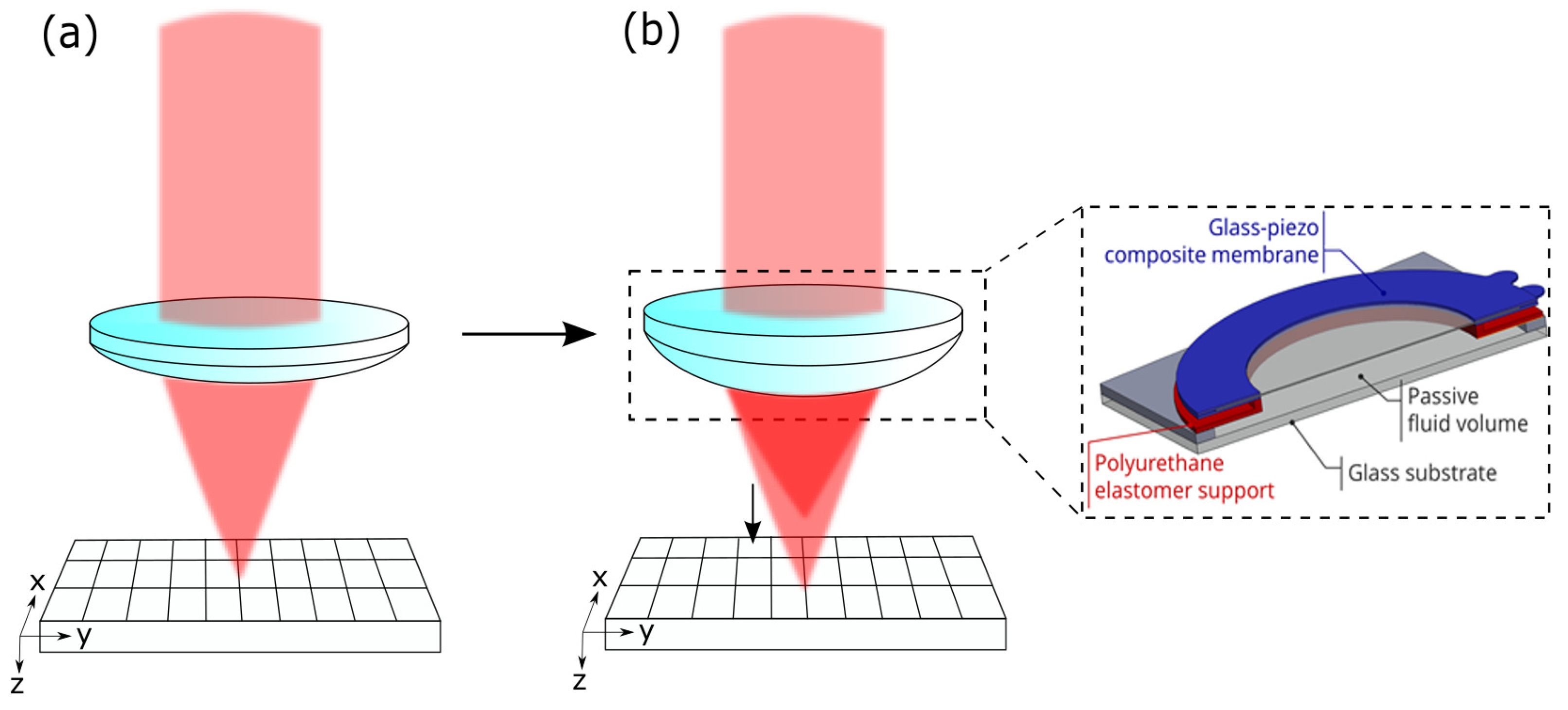
For axial scanning, the focal spot has to be shifted in the axial direction through the sample. To achieve such a shift, the AL induces a difference of the optical path length ($OPL$) when a beam is passing through the lens. Here, the $OPL$ is defined according to Equation (1), where n is the refractive index of the lens material and s is the length of the path through the lens:

$$OPL=n·s$$

(1)

TAG lenses achieve this by using sound energy to change the refractive index of the medium inside the lens [11], while the length s is constant. The alternative to a change of the refractive index is to adjust the local thickness of the lens by the deformation of the AL membrane with piezo actuators [14]. Such lenses enable high-speed axial scanning without the need for mechanical movement of the stage or microscope objective. However, environmental influences have a huge impact on the behavior of the AL. Therefore, it is necessary to monitor the behavior of the lens while scanning and to always be aware of the current position of the focal spot.

The control of AL with higher degrees of freedom, such as the lens with spherical aberration correction capabilities introduced in [14], becomes more challenging as the axial position of the focal plane varies based on unknown or non-linear dependencies. If such an AL is inserted into an optical setup closed-loop control supported by wave, front measurements can be used for control. There, the voltage is iteratively refined until the desired behaviour is reached. However, this is time-consuming, and the sample is exposed to the laser for a significant amount of time, hence, photobleaching might pose a problem.

To overcome these limitations we introduce a computational approach to estimate the current position of the focal plane while scanning and without iterations in the scanning process. The strategy is to monitor the behaviour of the scanning AL with a camera and assign the axial position to the recorded measurement point.

In several use cases, techniques of deep learning were able to solve non-linear problems better than a classical closed loop control [16]. Neural networks as a method of deep learning are able to consider a huge amounts of information with unknown importance [17]. Furthermore, a neural network avoids time-consuming iterations once it is trained, and photobleaching is expected to be strongly reduced.

For focal length estimation, different approaches based on images are implemented in the form of convolutional neural networks (CNN). It is possible to deal with the above-mentioned issue by calibration using specific patterns on a single image [18,19,20] or the usage of an RANSAC-based algorithm [21]. All these approaches have in common that a specific pattern must be visible on the image, so that the focal length is calculated based on the geometric features of this pattern. In addition, some techniques require more than one image to estimate the focal length [18], so no single shot estimation is possible. There are also newer approaches with deep learning in the form of neural networks to estimate the focal length from a single image without specific patterns [22,23,24,25]. However, all the above-mentioned methods were only applied on pictures of subjects such as landscapes, persons, animals, cells, or synthetically generated images. In the case of microscopy, it is beneficial to be independent from the type of sample. To our knowledge, there is currently no neural network to estimate the focal shift introduced by adaptive optics based on images without a subject on it available [22,23,24,25].

2. Experimental Setup

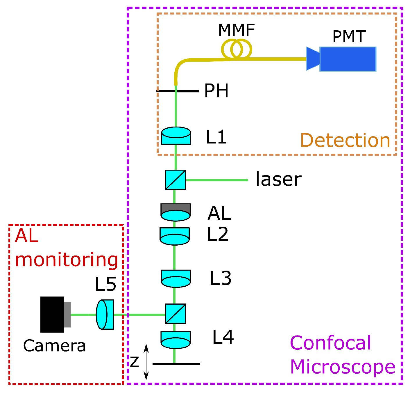
For training the CNN, we use experimental data. Therefore, we use a home-built confocal microscope setup, as shown in Figure 1. The laser source is a Thorlabs CPS532 laser with $4.5$ mW power operating at a wavelength of $\lambda =532$ nm. The beam passing the AL and the lenses L2 and L3 is divided by a beamsplitter into the measurement and the monitoring beams. The monitoring beam is directed onto a camera through lens L5, where the input image for the CNN is captured. L4 (Ashperical Lens 354453, Thorlabs Inc., Bergkirchen, Germany) focuses the measurement beam into the region of interest. Here, an aspherical lens was used as a front lens.

For calibration, a mirror which is located on a movable stage (stage controller XPS-Q8 and motorized actuators LTA-HS, Newport Corporation, Irvine, CA) is used as a sample. This stage is movable in three axes, but for the data acquisition, it has only been moved in the axial z-direction. The lenses L2 and L3 form a 4f-system that images the AL close to L4, which minimizes aberrations of the adaptive lens but still offers a high tuning range as described in [26].

The reflected light goes back, passing the 4f-system, is focused through the pinhole ($d=5$$\mathsf{\mu }$m from Thorlabs Inc.), and is measured with a detector (HCA-S Femto, Berlin, Germany). The light originating from out-of-focus regions is blocked by the pinhole. When the mirror is driven through the focus, the intensity distribution measured on the detector gives both the focus position and the axial resolution. If the voltage applied on the AL is changed, the peak of the intensity is shifted, and the focus position can be determined. The working principle of the AL is shown in Figure 2.

Assuming the lateral resolution in a confocal microscope to be defined as in Equation (2) and the axial resolution as in Equation (3) from [27]:

$$\Delta x,\Delta y=\frac{0.51·\lambda }{N{A}_{AL}}$$

(2)

$$\Delta z=\frac{0.64·\lambda }{n-\sqrt{n^2-N{A}_{AL}^2}}.$$

(3)

With $\lambda =570$ nm as the average wavelength of emission and excitation (defined by Equation (4)), n is the refractive index and $N{A}_{AL}$ is the numerical aperture. $N{A}_{AL}$ can be derived from Equation (5), here, this is the numerical aperture, which changes when a voltage is applied to the AL (induced by a change of the focal length $f_{obj}$) [27]:

$$\lambda =\sqrt{2}·\frac{{\lambda }_{ex}·{\lambda }_{em}}{\sqrt{{\lambda }_{ex}^2+{\lambda }_{em}^2}}$$

(4)

$$N{A}_{AL}=n·sin\left(\alpha \right)=n·sin\left(arctan\left(\frac{f_{obj}}{r}\right)\right)$$

(5)

Here, the refractive index is assumed as $n=1$, r is the half size of the spot in front of L4, and $f_{obj}$ is the focal length behind L4, influenced by the AL ($f_{obj}=4.61$ mm while 0V applied). The spot size of the laser beam is $d=10$ mm, so r is 5 mm; thereby, $NA$ is calculated as $0.68$. So, the lateral resolution becomes $0.4\mathsf{\mu }$m, and the axial resolution is $1.4\mathsf{\mu }$m. The radius of the Airy disk can be calculated according to Equation (6) [27]:

$$r_{Airy}=\frac{0.61·\lambda }{N{A}_{AL}}.$$

(6)

This leads to a radius of the Airy disk of $0.5\mathsf{\mu }$m:

$$r_{PH,proj}=\frac{r_{PH}}{M}.$$

(7)

$$AU=\frac{r_{PH,proj}}{r_{Airy}}.$$

(8)

M is the overall magnification of the setup, which can be stated as $10.7$, $r_{PH}$ is the size of the pinhole. Thereby, $r_{PH,proj}$ and the Airy Unit $AU$ are according to Equations (7) and (8) from [27 $0.46\mathsf{\mu }$m and $0.89\mathsf{\mu }$m.

The standard deviation of the focus position upon repeated application of a voltage on the adaptive lens at changing environmental conditions was found to be in the order of $50\mathsf{\mu }$m. To obtain a ground truth (gt) value for the current axial position of the focal spot, when a certain voltage is applied to the lens, the following procedure was performed. After applying a voltage to the AL, the stage was moved axially, and simultaneously, the intensity at the detector was recorded. The axial position of the focal spot was afterwards calculated as the position of the stage when the maximum intensity was measured at the detector. The axial resolution of the microscope is therefore crucial for the accuracy of the gt value.

3. Training of the Neural Network

Our network uses images captured from the monitoring beam of our CM setup. Hence, the position estimations are independent from the investigated sample. We use only experimental data to build a dataset for the network training, and this leads to an exceptionally small dataset.

Each data element in the dataset consists of an image from the illumination beam and the gt value of the axial focal spot position. To obtain a dataset for training, validation, and testing, for each element, the voltage AL is changed and the capturing procedure is repeated.

We use the AL introduced in [15] and apply voltages between 0 V and 20 V, resulting in an axial scanning range of $230\mathsf{\mu }$m.

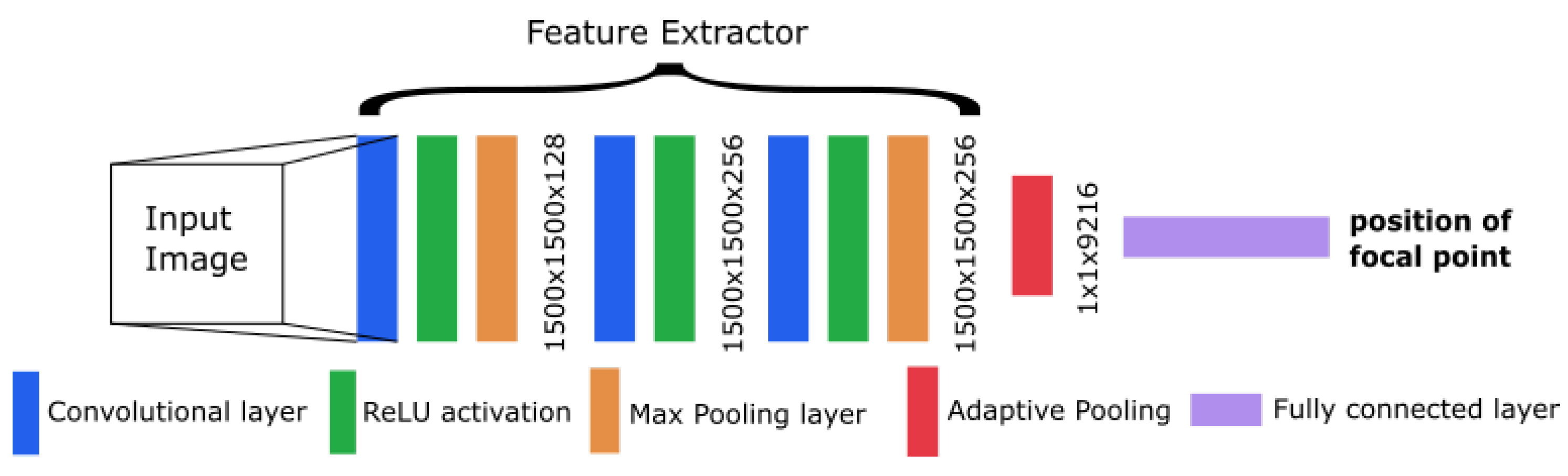
The CNN from Workman et al. [22] showed good performance in focal length estimation by using the feature extractor from AlexNet [28]. We also adapted this extractor into our model with some changes in the architecture. This results in a modified AlexNet with a different concept than the original network. To decrease the number of weights and speed up the training, we dropped some layers (including the dropout layers) from the original extractor. At the end of our architecture, we inserted one linear layer with a single output to obtain the focal length as a single number. An overview of the resulting architecture is shown in Figure 3.

3.1. Implementation Details

Our implementation is written with PyTorch Lightning framework [29]. This framework improved the comprehensibility of our code and simplified the training process. As a loss function, we decided to implement the mean squared error ($MSE$) between the estimated and ground truth focal length. The expression for $MSE$ is given in Equation (9):

$$MSE=\frac{1}{N}\sum _{i=1}^N{(x_{estimated}-x_{gt})}^2$$

(9)

where $x_{estimated}$ is the focal length estimated by the network and $x_{gt}$ is the annotated gt focal length, while N is the number of elements used for the calculation. This loss calculation has the advantage that large deviations of the estimated value from the ground truth value have a larger weight. Small deviations are weighted as less intense but still allow the loss to converge over epochs.

To obtain a better understanding for the difference between the gt and the estimated value as an alternative, the mean absolute error ($MAE$) can be used. The $MAE$ is defined as average difference, see Equation (10):

$$MAE=\frac{1}{N}\sum _{i=1}^N|x_{estimated}-x_{gt}|$$

(10)

To clarify the test loss, we use the $MAE$ in addition to the $MSE$ as a metric. The results on the test-dataset are provided in

Table 1. Results of the trained CNN on the test dataset; TF = transfer learning; $MSE$ = mean square error; $MAE$ = mean average error; $STD$ = standard deviation.

	$\mathit{MSE}$ [$\mathsf{\mu }$m${}^2$]	$\mathit{MAE}$ [$\mathsf{\mu }$m]	$\mathit{STD}$ [$\mathsf{\mu }$m]	Accuracy [%]
1st Dataset	53.61	6.5	3.88	75
2nd Datset before TF	48,486.00	213.36	62.85	0
2nd Dataset after TF	69.59	8.15	2.01	75

.

3.2. Training Procedure

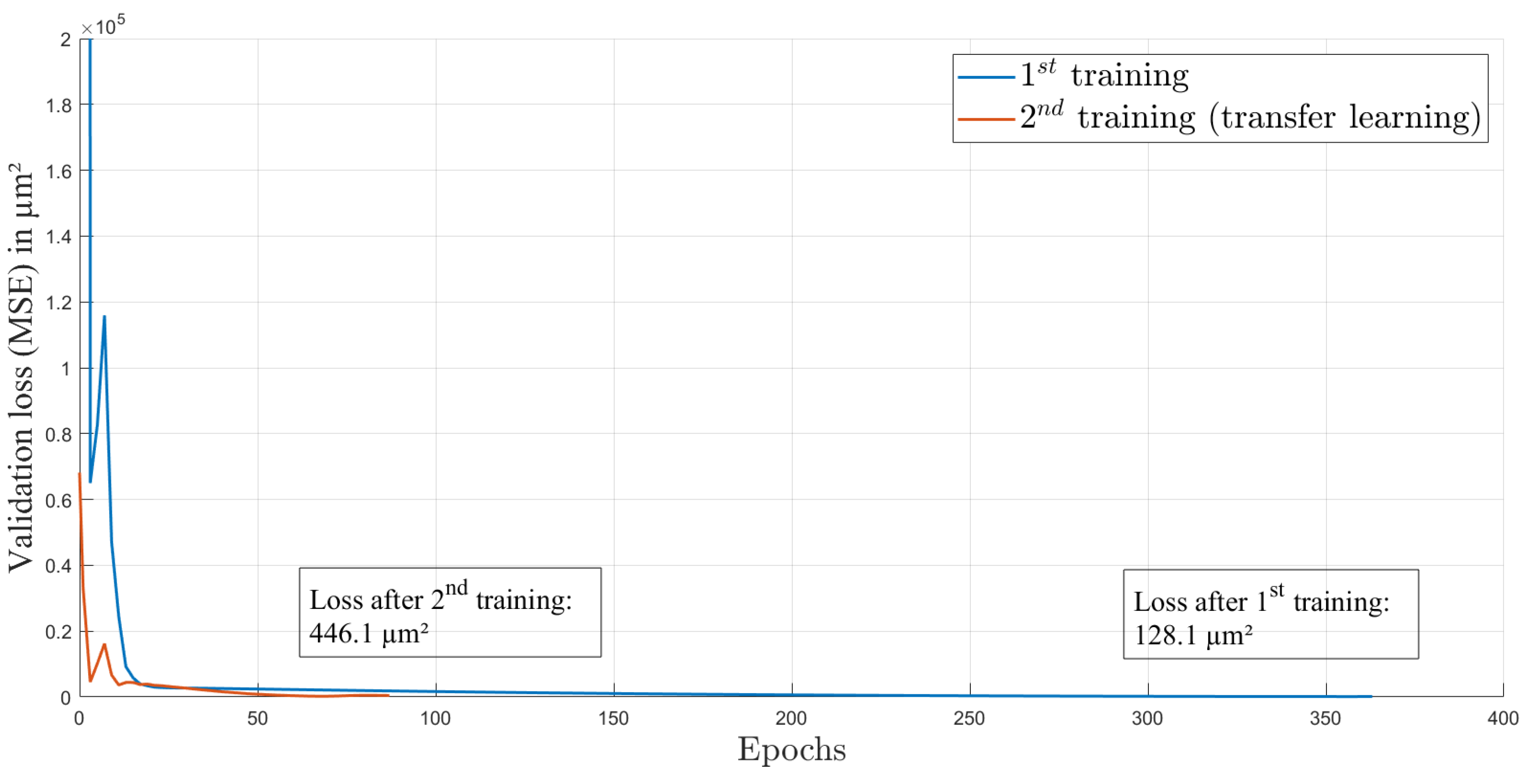
For training, we used an Adam optimizer and an initial learning rate of 1.995 × 10${}^{-4}$. This learning rate was calculated by the learning rate finder from PyTorch Lightning framework [29]. The optimal learning rate is at the point of highest initial descent of training loss and provides an optimal start of the training process. The loss function over the 363 epochs of the first training is shown in Figure 4. The curve is rapidly decreasing in the first epochs and afterwards is decreasing more slowly. This behavior is expected and indicates a successful training process. The split of the dataset into the training and validation datasets is 60:40, with 37 elements in total. Each element contains one image and one ground truth value of the axial focal spot position.

Additionally, we used four elements as test-set; please take note that there was no data augmentation added to the test set, and the elements were completely unknown to the CNN. The dataset is comparably small because all elements in the dataset were annotated by hand. Often, synthetic data are created by simulations to obtain large datasets for training. However, here, we had no model available that could adequately produce synthetic data and take into account experimental and environmental influences. However, as it is shown in Section 4, even on a small dataset a successful training is possible and can achieve satisfying results.

However, increasing the used data may offer slightly better results, but in future steps, it is planned to face highly increased difficulties, as more complex adaptive lenses will be used, with two or more input voltages, e.g., for additional aberration correction. Then, phase measurement has to be included into the setup, which will strongly increase the complexity. Thus, the dimension of the dataset will also be increased to address the extended set of features. These features will also include a high variety of aberrations. Hence, it is fundamental to keep the complexity at this stage as low as possible, thus the used number of data was suitable to reach the targeted estimation quality. An adequate CNN-based solution is the only way to make the adaptive optical component-based microscopy competitive.

4. Experiment and Results

In the last epoch of training (epoch 363), our model estimates the focal length on the validation data as $MSE$ of $128\mathsf{\mu }$m${}^2$ from the corresponding ground truth on the validation data. Furthermore, random noise was added as data augmentation to the validation and training datasets, but for testing, a small dataset without data augmentation was used. For data augmentation, Gaussian noise from [30] was used. Here, noise in the form of counts was added to each pixel per image. The noise was sampled from a normal distribution with a mean of zero counts and a standard deviation of eight counts for the first training process. Thereby, it was possible to enhance the dimension of the training and validation datasets to 13,431 images. On this test dataset, we end up with a test loss of $6.5\mathsf{\mu }$m, calculated as $MAE$. This test loss depends on the overall performance of the network and its hyper-parameter but also on the quality and quantity of the training data. The training was performed on a system consisting of AMD Ryzen 9 3900X 12× 3.80 GHz (CPU) and Corsair DIMM 128 GB DDR4-2666 Quad-Kit (RAM) and GeForce RTX 2080 Ti Blower (GPU). Here, the first training took 69 min.

To prevent our model from overfitting and to achieve a good generalization, we used the following strategies:

• Early stopping after four validation epochs without decreasing validation loss;
• Data augmentation (random noise) [30].

To assess the results of an experimental application of the CNN in combination with the AL, measurement uncertainties should be considered first. As potential sources of uncertainties in the setup, we identified the movement stage and random measurement uncertainties while capturing the gt values and camera parameters.

The motorized stage has an unidirectional repeatability of $0.25\mathsf{\mu }$m and provides minimum incremental motion of $0.1\mathsf{\mu }$m [31]. These tolerances are far below cell size ($10\mathsf{\mu }$m), thus, we neglect these influences. To minimize random measurement uncertainties with unknown origin, we used the average of 10 axial scans to obtain the gt value of the position of the focal plane. The camera parameters have a huge impact on image quality criteria such as the saturation of pixels, etc. The quality of the images for the CNN is an important factor for the learning process. Additional changes in the images through unsuitable camera parameters might make a correct estimation more difficult to achieve. To deal with this problem, we used the automatic mode for camera usage to avoid over saturation and other issues.

For complex specimens, sample-induced aberrations may be an issue that could degrade the performance quality, as the focus position estimations of the CNN are made independent of the sample.

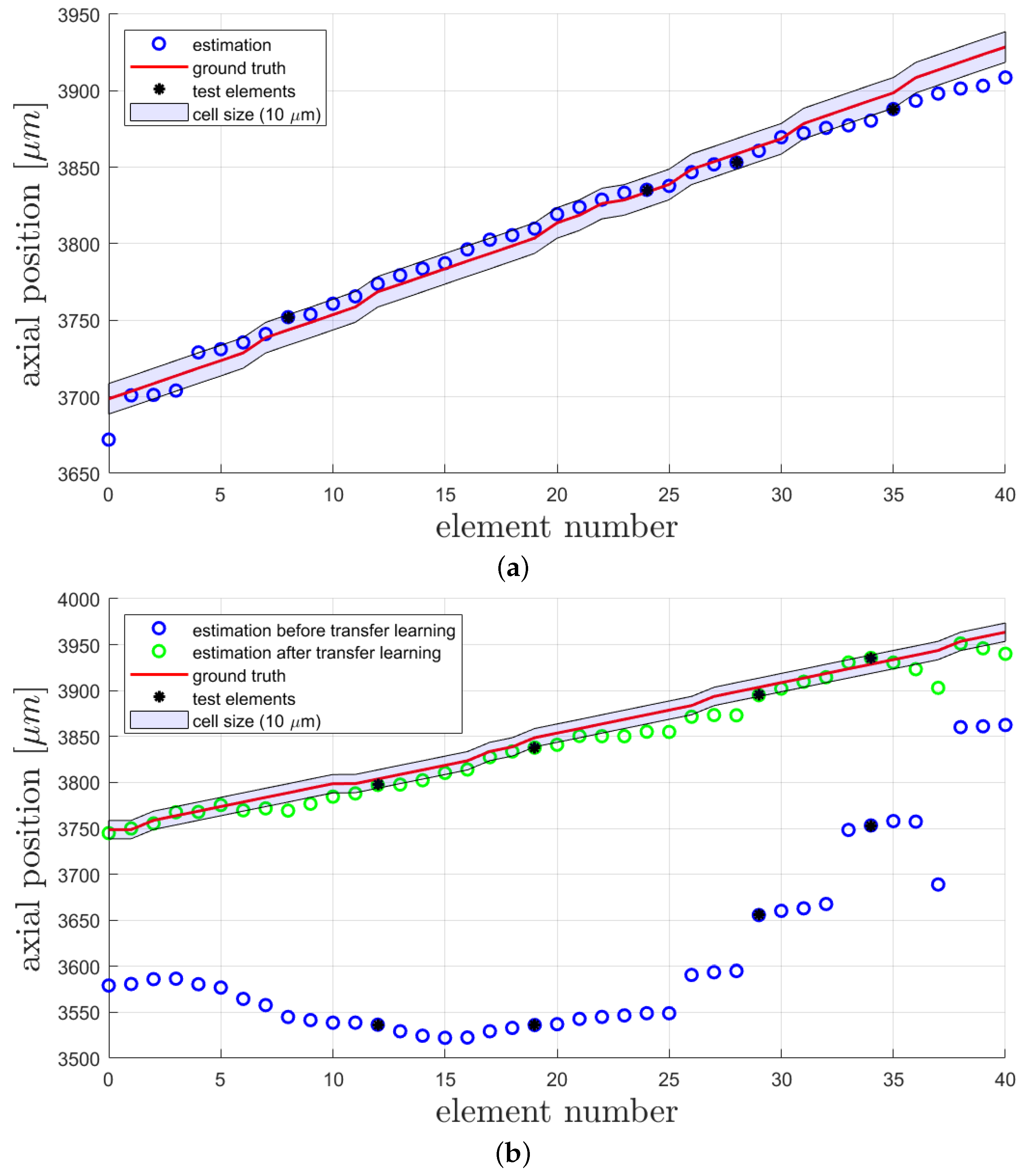
To investigate the quality of the estimations made by the CNN, loss functions and accuracy calculations are a common method of evaluation. In Figure 5a, the gt values and estimated values for each data element in the training, validation, and test sets are shown.Here, the estimations of the trained CNN on all available data elements are shown. Of course, the elements for testing were not included in the training process; there, only training and validation elements were used. The elements from the test set are marked with a black star. Our main goal was to achieve a precision of $10\mathsf{\mu }$m (average size of thyroid cells in zebrafish according to [14]), and to illustrate this, a shade around the gt with this width is added. From this image, one can see that this goal is mainly achieved for the middle elements, while the elements in the beginning and the end are differingly stronger. Elements at the beginning and the end are linked to a very low or very high voltage and so to the clearest distortion in the input image for the CNN. It is possible that learning features in the middle of a range is easier for the CNN, and this might depend on the camera parameters used and the possible occurrence of over saturation at the end of the range. However, due to the test loss of $6.5\mathsf{\mu }$m ($MAE$), our CNN obviously shows a good performance inside the desired range of tolerance. The statistical results on the test datasets are summarized in Table 1. Here, the accuracy of the results on the test dataset consisting of four elements is also reported. Each estimation, which differs less than $10\mathsf{\mu }$m from the ground truth value, is considered as a correct estimation.

After several weeks and some lens adjustment, another dataset from the same setup and also consisting of 41 data elements was recorded to investigate the performance of the network on data after the AL was influenced by environmental circumstances such as changing ambient temperature and pressure. We used four random elements of this dataset for testing with the trained network and reached a test loss of $213.36\mathsf{\mu }$m ($MAE$), see Table 1. As shown in Figure 5b (blue circles), the estimations do not match the corresponding gt values anymore. This is caused by the intentional misalignment of the setup, leading to different gt values compared to the first dataset. Here, the elements from the test dataset are marked in black. The test elements were not included in the training or validation process. We used transfer learning [32] to improve the performance, and again, data augmentation was used to extend the dataset. As in the first training process, Gaussian noise was added to the images, but here, the noise was sampled from a normal distribution with a standard deviation of 10 counts. This enables the extension of the training and validation data to 3219 images. In the method of transfer learning, a trained CNN is again trained with a slightly different dataset on top. This enables the CNN to recognise input elements with small discrepancy compared to the first dataset. After 87 epochs of transfer learning with heavier data augmentation than in the first training, the CNN achieved a test loss of about $8.15\mathsf{\mu }$m ($MAE$). The whole process of transfer learning was conducted with the second dataset, which was recorded several weeks after the first dataset. The validation loss while training is provided in Figure 4. The improvement in correctness of the network estimations can also be seen in Figure 5b, where the estimations after transfer learning are displayed with green circles and the test elements are marked in black. It is obvious that some pattern of estimation distribution from before transfer learning are still visible in the estimations after transfer learning. By comparing the mean difference ($MAE$) of gt and estimation before transfer learning ($213\mathsf{\mu }$m) and after transfer learning ($8\mathsf{\mu }$m), a huge improvement is shown. Furthermore, the standard deviation ($STD$) of the difference also decreased from $62\mathsf{\mu }$m before transfer learning to $2\mathsf{\mu }$m afterwards. The transfer learning process took 16 min on the above-described system.

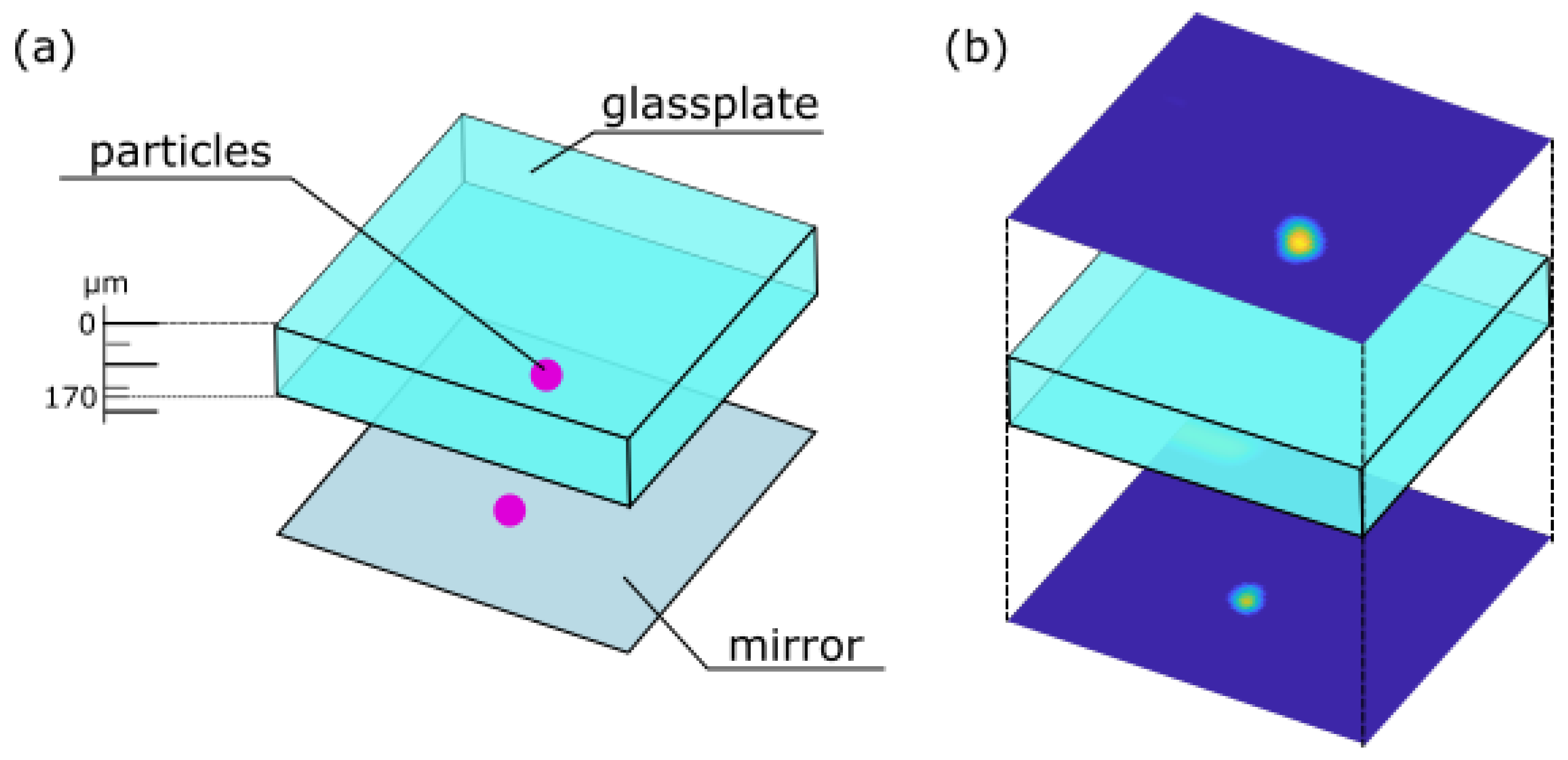
As an exemplary application, a scan through a fluorescent specimen was performed. In Life Sciences, the investigation of fluorescent specimen by using confocal microscopy is a principal task [33]. To prepare a fluorescent sample fluorescent beads were placed onto a mirror, followed by a microscope slide where on top again fluorescent particles were located. A scheme of this sample is shown in Figure 6a.

For measurement of the fluorescent light with the detector, a longpass filter with the cut-on wavelength 550 nm (Thorlabs FEL0550) was placed between lens L1 and the upper beam splitter. Furthermore, a voltage amplifier (Femto DLCPA-200) and another photosensor (Hamatsu H10720-20) were necessary to improve the detection, filter the noise, and detect the fluorescent signal.

The fluorescent beads are detected by performing lateral scans of the above introduced sample, the resulting lateral scans are shown in Figure 6b. The lateral scans were performed using a movable stage actuated by a Newport XPS system (for details see Section 2). Thereby, the y-axis was used as the slow axis, while the x-axis was used as the fast axis. An axial shift in the z-axis was only achieved due to tuning the voltage applied to the AL. The scans originate from different axial positions above and underneath the glass plate. Simultaneously, the lateral scans images from the illumination beam were captured. These images serve as input images for the trained CNN.

The estimations made by the CNN for the in-focus particles are then subtracted to obtain the thickness of the plate in the sample. In this case, the difference of the estimations is $169\mathsf{\mu }$m, and the ground truth optical pathway is $170\pm 5\mathsf{\mu }$m. So, the length through the glass plate with fluorescent particles on top of the mirror and the glass was estimated properly.

5. Conclusions

We presented a modified implementation of the AlexNet architecture for a neural network to estimate the position of the focal plane in an adaptive confocal microscope based on an image of the illumination beam. With this network, it is possible to perform accurate single shot estimation of the focal spot position with an $MAE$ under $10\mathsf{\mu }$m, which is the average size of thyroid cells in zebrafish embryos. In previous studies, zebrafish thyroids have already been investigated by adaptive lens scanning.

As a practical application of the network, we reported a thickness measurement of a sample with fluorescent beads, which was performed by our network and the adaptive lens replacing a movable stage. One of the main advantages here is the independence of samples. This is possible because the neural network takes an image from the illumination beam before surpassing the sample as input. So no information from the sample is included in the image for the CNN. Thus, the type of sample is irrelevant for the CNN and makes it quite versatile. However, the network parameters and architecture might have to be adapted for data from other experimental setups. The challenge here is to find the optimal training parameters and grade of data augmentation. However, several rounds of transfer learning should enhance the robustness and generalization ability of the CNN. So, the fine tuning of the training parameters might become less crucial.

Although we had to challenge a small dataset for training and measurement uncertainties, it was possible to develop and train a CNN for single shot focal point estimation in a confocal setup. With this work, we placed a cornerstone for smart microscopy and made a step forward to fast self calibration for adaptive optics.