Lossless Compression of Sensor Signals Using an Untrained Multi-Channel Recurrent Neural Predictor

Abstract

The use of sensor applications has been steadily increasing, leading to an urgent need for efficient data compression techniques to facilitate the storage, transmission, and processing of digital signals generated by sensors. Unlike other sequential data such as text sequences, sensor signals have more complex statistical characteristics. Specifically, in every signal point, each bit, which corresponds to a specific precision scale, follows its own conditional distribution depending on its history and even other bits. Therefore, applying existing general-purpose data compressors usually leads to a relatively low compression ratio, since these compressors do not fully exploit such internal features. What is worse, partitioning a bit stream into groups with a preset size will sometimes break the integrity of each signal point. In this paper, we present a lossless data compressor dedicated to compressing sensor signals which is built upon a novel recurrent neural architecture named multi-channel recurrent unit (MCRU). Each channel in the proposed MCRU models a specific precision range of each signal point without breaking data integrity. During compressing and decompressing, the mirrored network will be trained on observed data; thus, no pre-training is needed. The superiority of our approach over other compressors is demonstrated experimentally on various types of sensor signals.

1. Introduction

As digitalization advances continuously, sensor technology is undergoing tremendous development and has been widely used in applications such as wearable medical devices [1], climate change tracking [2], and infrastructure monitoring [3]. At the same time, with the improvement of the resolution and sampling rate of analog-to-digital converters (ADCs), the volume of sensor signals increases rapidly, leading to great pressure on data storage. One way to alleviate such pressure is to reduce the redundancy existing in massive data through data compression. Data compression techniques can be categorized into two classes: lossless compression and lossy compression. Lossy compression of sensor signals discards part of the secondary information, and the resulting distortion is limited within an acceptable range. For example, An et al. proposed a data compression method based on two-dimensional discrete cosine transform (DCT), which can effectively reduce the amount of data since most natural signals are concentrated in the low frequency parts of DCT [4]. Zhang et al. proposed a compression method based on wavelet transform and obtained a high signal-to-noise ratio [5]. These methods can produce a high compression ratio at the cost of dropping part of the signal information. However, in many scenarios, such as sensor debugging [6], sensor signals must be stored losslessly. In such cases, lossless data compression is used. For example, Biagetti et al. explained the importance of lossless compression algorithms in electromyography (EMG) sensors and analyzed the energy consumption and performance of existing lossless compressors [7].

Classical general-purpose lossless compression algorithms mainly include entropy coding and dictionary coding. The former is based on Shannon information theory [8], including Huffman coding [9], arithmetic coding [10], and asymmetric numeral systems (ANS) [11]. The later is based on LZ algorithm and its variants, which compress data by replacing repeated data with the earlier position of that data in the uncompressed stream [12,13]. To better utilize the context information underlying sequential data, context-based compression methods were proposed. The general idea of these methods is to combine a context-based predictor and a coding algorithm. Among context-based algorithms, PAQ uses a large number of models conditioned on different contexts (e.g., n-grams, sparse contexts, analog contexts, etc.) to estimate the probability distribution of the next symbol [14]. Deep learning models are naturally context extractors, which can be used as effective probabilistic predictors in context-based compressors. Byron proposed CMIX [15], which uses a large number of context models including a long short-term memory (LSTM) [16]. Goyal et al. proposed DZip [17], which uses a pre-trained neural network as a predictor, which is stored in the compressed file after compression. Different from DZip, tensorflow-compress [18] trains its deep learning predictor during compressing and decompressing; thus, it does not need to store the model parameters and can run with a large batch size to get a substantial speed improvement.

The compressors mentioned above are general-purpose methods which perform data compression by reducing the redundant information between data points. For sensor signals, this inter-point relationship may be the continuity and periodicity. However, sensor signals also have intra-point features. Specifically, each bit in every signal point has its own underlying conditional distribution, depending on the history values of its own and other bits. For example, the values of lower-order bits change more frequently than values of higher-order bits. Therefore, applying general-purpose compressors directly to sensor signals often leads to a relatively low compression ratio, since they do not fully exploit the intra-point characteristics mentioned above. What is more, most of the general-purpose compressors read a fixed number of bits at a time. In this way, a bit stream of a sensor signal will be partitioned into groups before being fed into the compressor, which may break the data integrity of sensor signals. There are also compressors that are specially designed for digital signals. Dai et al. proposed a lossless compression method for periodic signals based on an adaptive dictionary model which can predict the current data value according to the history [19]. Huang et al. proposed a novel ECG signal prediction model that uses an autoregressive integrated moving average (ARIMA) model and discrete wavelet transform (DWT) [20]. Nonetheless, these compressors are all designed for specific signals.

In this paper, we present a novel recurrent neural network (RNN) architecture that is specially designed for modeling sensor signals as the probability predictor of a context-based lossless compressor. The proposed multi-channel recurrent unit (MCRU) reads one signal point at a time, and the internal bits are re-grouped into multiple channels, each of which is assigned with a sub-recurrent unit. In this way, the intra-point features can be extracted without breaking the integrity of each signal point. Furthermore, we adopt a similar strategy as tensorflow-compress to train the network during compressing and decompressing; thus, no pre-training is needed. The effectiveness of the proposed approach is demonstrated experimentally on different types of sensor signals.

2. Context-Based Lossless Compression for Sensor Signals

In this section, we first introduce the basic logic of sequence prediction for digital signals. Then, the general framework of context-based lossless compression algorithms, on which the proposed method of this paper is based, is presented. For mathematical notations, we denote the vectors and matrices by bold lower- and upper-case letters, respectively, e.g., $\mathbf{x}$ and $\mathbf{W}$. Functions are denoted by upper-case letters in calligraphic font, e.g., $\mathcal{F}$.

2.1. Digital Signals and Sequence Predictor

A digital signal $\left\{s_i\right\}$ of length L sampled by an $R_a$-bit ADC is stored as a sequence of bits $\left\{b_j\right\}$ in hardware:

$$\underset{s_1}{\underbrace{b_1^{s_1},\cdots ,b_{R_a}^{s_1}}},\underset{s_2}{\underbrace{b_1^{s_2},\cdots ,b_{R_a}^{s_2}}},\cdots ,\underset{s_L}{\underbrace{b_1^{s_L},\cdots ,b_{R_a}^{s_L}}},$$

(1)

where $R_a$ is the ADC resolution, and $b_j^{s_i}\in \{0,1\}(1\le i\le L,1\le j\le R_a)$ denotes the j-th bit in the i-th sampled value. In this paper, we assume that the order of bits in each sampled value is ascending, i.e., $b_1^{s_i}$ and $b_{R_a}^{s_i}$ represent the lowest- and highest-order bits in $s_i$, respectively.

On the other hand, a sequence predictor $\mathcal{Q}$ predicts future values based on previously observed values by modeling relationships between data points in a data series $\left\{x_t\right\}$. At time step t, $\mathcal{Q}$ regards the value to be predicted as a random variable ${\xi }_t$, and gives a probability distribution over all its possible values $\{v_1,\cdots ,v_N\}$:

$$\mathrm{Pr}({\xi }_t=v_i|x_1,\cdots ,x_{t-1}),i=1,\cdots ,N,$$

(2)

where $x_1,\cdots ,x_{t-1}$ are previous observations. Given a digital signal $\left\{s_i\right\}$, a sequence predictor usually predicts $R_p$ bits at a time by re-grouping the bit sequence in Equation (1) to $\left\{x_t\right\}$. In this way, each $x_t$ has a total of $2^{R_p}$ possible values, i.e., in Equation (2), $N=2^{R_p}$. In the following discussion, we refer to $R_p$ as the predictor resolution.

In this paper, we use bits per character (BPC, [21]) to measure the performance of a sequence predictor. Note that for digital-signal predictors, the BPC on a re-grouped sequence $\left\{x_t\right\}$ of length T is calculated as

$$-\frac{8}{T{R}_p}\sum _{t=1}^T{log}_2\mathrm{Pr}({\xi }_t=x_t|x_1,\cdots ,x_{t-1}).$$

(3)

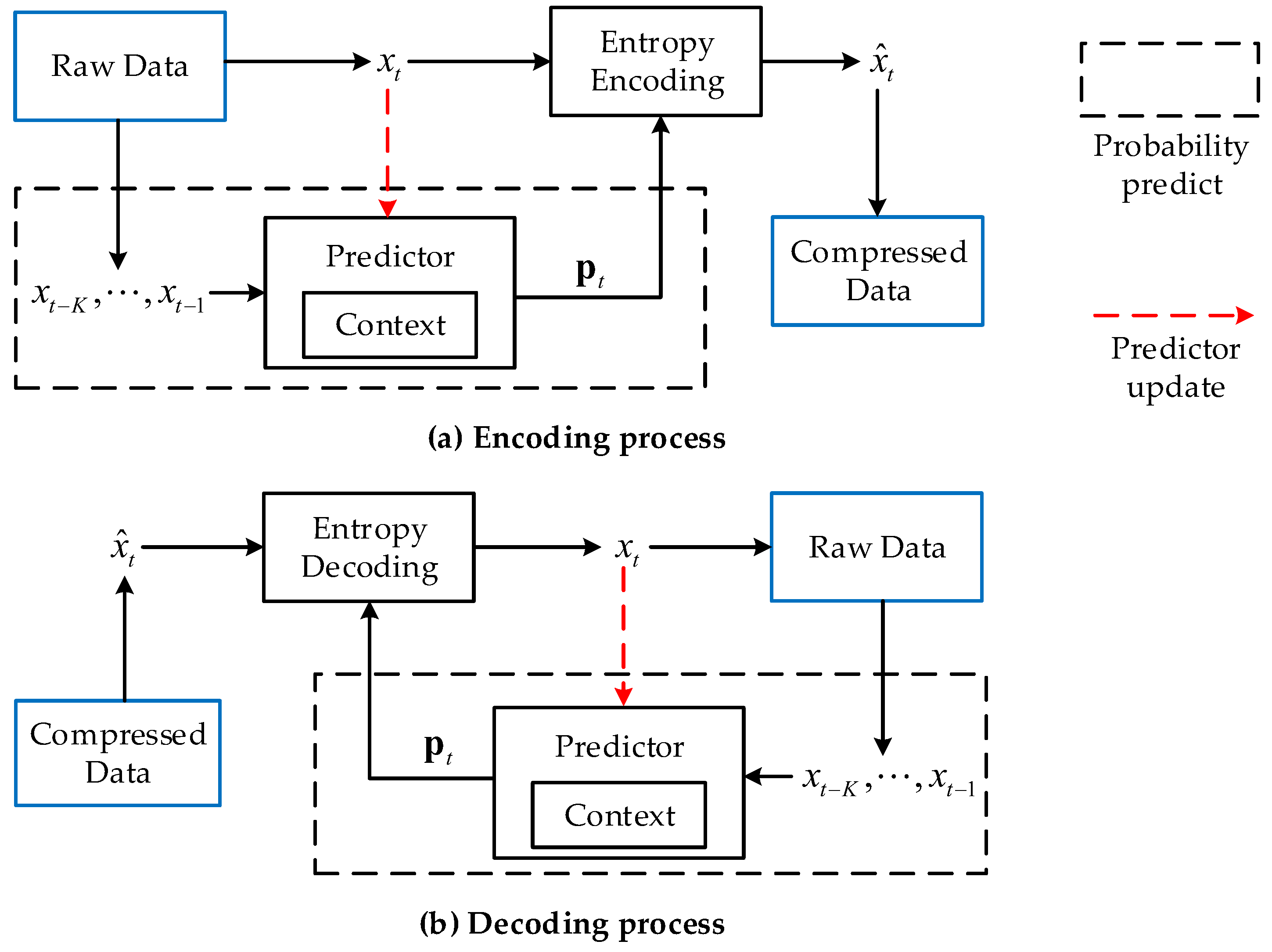
2.2. Context-Based Encoding and Decoding

The proposed approach in this paper is built upon a context-based lossless compression framework which consists of a predictor and a coding module. Specifically, we use entropy coding as the coding module, and a sequence predictor is used to give the probability prediction, as in Equation (2). Here we summarize the general flow of such a context-based encoding and decoding scheme, as shown in Figure 1. At each encoding/decoding step t, the predictor first reads K latest data points $\left\{x_{t-K},\cdots ,x_{t-1}\right\}$ from raw data and gives a prediction ${\mathbf{p}}_t$. This prediction is then sent to the entropy coding module to encode raw data $x_t$, or decode compressed data ${\widehat{x}}_t$. For some context-based compressors, the predictor will be updated based on the true value, i.e., $x_t$, of the prediction made. In this paper, all mentioned context-based compressors, including the proposed approach, use arithmetic coding [10] as the entropy coding module, unless otherwise specified.

Among the context-based approaches, the ones based on the LZ77 algorithm [12], which uses a dictionary to maintain the context of data, are perhaps the most widely used. For example, the famous compression tool Gzip, to which our proposed method is compared in Section 4, is based on LZ77 and Huffman coding [9]. Another popular LZ77-based compressor, namely LZMA, uses arithmetic coding as the entropy coding module. These compressors work without the prior knowledge of the data to be compressed. In addition, they are not able to model the underlying joint distributions of data points, leading to a relatively low compression rate (see

Table 1. The CR results of the tested compressors.

Name	Gzip	BSC	PAQ	CMIX	Ours
BLOND-1	1.644	4.348	4.658	4.869	4.684
BLOND-2	1.627	4.215	4.508	4.753	4.577
BLOND-3	1.594	4.012	4.295	4.655	4.896
BLOND-4	1.600	4.107	4.418	4.651	4.487
BLOND-5	1.491	3.196	3.474	3.662	3.584
ESC-0	1.631	2.309	2.812	3.177	3.344
ESC-1	2.070	2.491	3.108	3.431	3.651
ESC-2	1.437	1.734	2.039	2.206	2.297
ESC-3	1.388	1.743	2.166	2.382	2.501
ESC-4	1.299	1.519	1.854	2.083	2.164
MPACT-DJI	1.357	1.564	2.117	2.342	2.390
MPACT-FlySky	1.367	1.863	2.142	2.457	2.553
MPACT-Futaba	1.399	1.904	2.162	2.472	2.564
MPACT-Graupner	1.382	1.892	2.204	2.477	2.560
MPACT-HobbyK	1.300	1.766	2.102	2.380	2.446
DJI-14bits	1.109	1.272	1.670	1.916	2.090
FlySky-14bits	1.103	1.420	1.777	2.004	2.219
Futaba-14bits	1.117	1.474	1.806	2.026	2.234
Graupner-14bits	1.144	1.407	1.792	2.037	2.230
HobbyK-14bits	1.083	1.303	1.659	1.924	2.156

). To address this issue, CMIX [15] combines a large number of context-based predictors, achieving a state-of-the-art compression ratio on several compression benchmarks [22,23] at the cost of slow compression speed.

Deep learning models, especially recurrent neural networks (RNNs), have been proven to be good at modeling context information hidden in sequential data. Naturally, they can be used as probability predictors in context-based compressors. DZip [17] uses a single deep learning model as the probability predictor. At each time step t, it calculates the conditional probability distribution based on previously observed K symbols. However, DZip requires pre-training the neural network, and the trained model is stored as a part of the compressed data in order to achieve a better compression rate. The aforementioned CMIX compressor also contains a deep learning predictor based on long short-term memory (LSTM, [16]). This sub-module is named lstm-compress, and can only work with a batch size of 1. Another deep learning-based lossless compressor, called tensorflow-compress [18], is a general version of lstm-compress, which can work with different recurrent units and an arbitrary batch size. Compared to the static DZip method, lstm-compress and tensorflow-compress do not require pre-training of their deep learning predictor; thus, they do not need to include the neural networks into the compressed data provided that both the compressor and the decompressor are initialized with the same random predictors. During encoding and decoding, the context information is extracted and stored in network state, and the RNN predictor is updated (indicated by red dashed line in Figure 1) via a standard back-propagation through time (BPTT, [24]) algorithm. In this paper, we refer to this kind of context-based technique as dynamic deep recurrent compressor (dynamic DRC).

Although the aforementioned compression techniques are promising, they can not fully exploit the special characteristics of sensor signals. For example, the predictor resolution $R_p$, defined in Section 2.1, is usually fixed to 8 in these general compressors. In the case that ADC resolution $R_a\ne R_p$, re-grouping the bit sequence will lose the original data property. Even though the predictor resolution can be arbitrary for some RNN-based compressors, setting $R_p$ to $R_a$ will result in formidable model sizes when the signal sequence is generated from a high-resolution ADC. To address these problems, we propose a new dynamic DRC with a novel recurrent predictor that is specially designed for compressing sensor signals. The network detail is presented in the following section.

3. Multi-Channel Recurrent Predictor

In this section, we present the proposed multi-channel recurrent predictor by first introducing the background of RNNs.

3.1. Recurrent Neural Networks

An RNN can encode a sequence of arbitrary length $\left\{{\mathbf{x}}_t\right\}$ into a fixed-sized state vector ${\mathbf{s}}_t$ by reading one data point at a time. In most cases, at each time step t, the state vector ${\mathbf{s}}_t$ will first be updated and then be used to calculate the model output:

$$\begin{array}{ll}\hfill {\mathbf{s}}_t& =\mathcal{T}({\mathbf{x}}_t,{\mathbf{s}}_{t-1}),\hfill \end{array}$$

(4)

$$\begin{array}{ll}\hfill {\mathbf{y}}_t& =\mathcal{G}\left({\mathbf{s}}_t\right),\hfill \end{array}$$

(5)

where $\mathcal{T}$ is the state transition function, $\mathcal{G}$ is the output function, and ${\mathbf{x}}_t$ and ${\mathbf{y}}_t$ represent the input and output vector of the RNN at time step t, respectively. One of the most fundamental building blocks of RNNs is the perceptron operator [25], which is defined as:

$$\begin{array}{cc}\hfill \mathcal{P}({\mathbf{u}}_1,\cdots ,{\mathbf{u}}_M;\varphi )& =\varphi (\mathbf{b}+\sum _{i=1}^M{\mathbf{W}}_i{\mathbf{u}}_i),\hfill \end{array}$$

(6)

where ${\mathbf{W}}_i$ is called the weight matrix relating to input ${\mathbf{u}}_i$, $\mathbf{b}$ is the bias vector, and $\varphi$ represents the non-linear activation function. The most simple RNN architecture simply uses a perceptron operator as the state transition function.

To alleviate the well-known vanishing and exploding gradient issue of RNNs, a gate unit is introduced [16], and the state transition function is constructed as a highway operator [25] $\mathcal{H}$, which can be generally defined as:

$$\begin{array}{cc}\hfill {\mathbf{s}}_t& =\mathcal{H}({\mathbf{x}}_t,{\mathbf{s}}_{t-1})={\mathbf{g}}_t^{\beta }\odot {\mathbf{s}}_{t-1}+{\mathbf{g}}_t^{\alpha }\odot {\widehat{\mathbf{s}}}_t,\hfill \end{array}$$

(7)

where ⊙ represents element-wise multiplication, ${\widehat{\mathbf{s}}}_t$ is a candidate state vector, and ${\mathbf{g}}_t^{\alpha }$ and ${\mathbf{g}}_t^{\beta }$ are gate vectors, in which each value is between 0 and 1. For example, candidate state and gate vectors in the popular gated recurrent unit (GRU, [26]) are calculated as:

$$\begin{array}{ll}{\widehat{\mathbf{s}}}_t\hfill & ={\mathcal{P}}_s({\mathbf{x}}_t,{\mathcal{P}}_r({\mathbf{x}}_t,{\mathbf{s}}_{t-1};\sigma )\odot {\mathbf{s}}_{t-1};tanh),\hfill \end{array}$$

(8)

$$\begin{array}{ll}{\mathbf{g}}_t^{\alpha }\hfill & ={\mathcal{P}}_{\alpha }({\mathbf{x}}_t,{\mathbf{s}}_{t-1};\sigma ),\hfill \end{array}$$

(9)

$$\begin{array}{ll}{\mathbf{g}}_t^{\beta }\hfill & =1-{\mathbf{g}}_t^{\alpha },\hfill \end{array}$$

(10)

where $\sigma$ and tanh represent the sigmoid and hyperbolic activation function, respectively. In this paper, we denote such a highway operator as ${\mathcal{H}}_{\mathrm{GRU}}$.

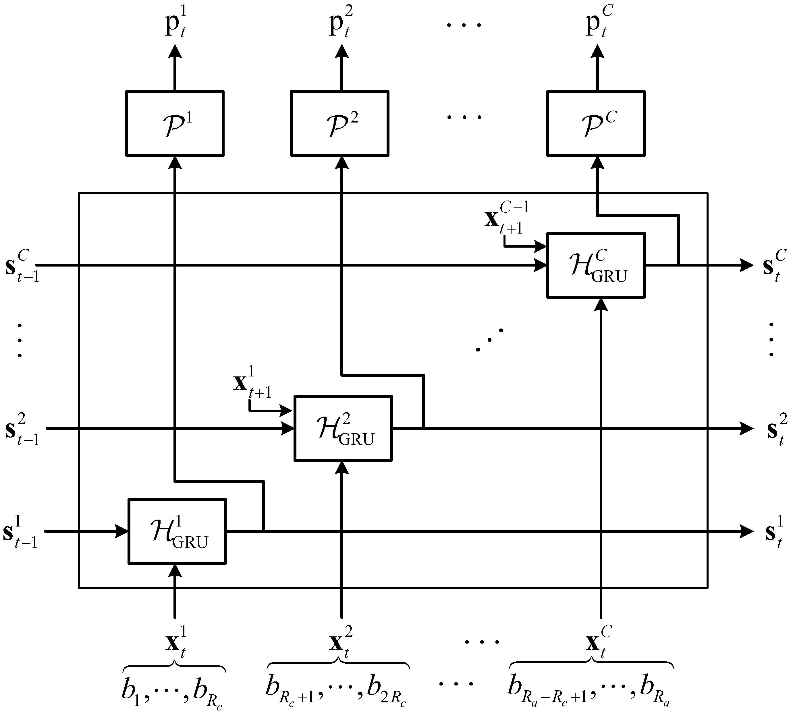
3.2. Multi-Channel Recurrent Unit

In this sub-section, we present a novel multi-channel recurrent unit (MCRU), which is specially designed as a deep-learning predictor for sensor signals. The predictor resolution $R_p$ is set to the ADC resolution $R_a$ in order to keep the integrity of each value sampled by ADC. Specifically, every $R_a$ bit is re-grouped into C channels, each of which corresponds to $R_c=\frac{R_a}{C}$ bits and represents a specific precision scale of the sample value. Each channel is assigned an independent ${\mathcal{H}}_{\mathrm{GRU}}$; thus, the context information of the corresponding precision scale is retained individually.

At each time step t, C predictions, namely, ${\mathbf{p}}_t^1,\cdots ,{\mathbf{p}}_t^C$, are made in order from less-significant-bit (LSB) channels to more-significant-bit (MSB) channels, as is illustrated in Figure 2. Specifically, for the j-th channel, the corresponding state vector is updated first:

$${\mathbf{s}}_t^j=\left\{\begin{array}{cc}{\mathcal{H}}_{\mathrm{GRU}}^1({\mathbf{x}}_t^1,{\mathbf{s}}_{t-1}^1),\hfill & \mathrm{if}j=1,\hfill \\ {\mathcal{H}}_{\mathrm{GRU}}^j({\mathbf{x}}_t^j,{\mathbf{x}}_{t+1}^{j-1},{\mathbf{s}}_{t-1}^j),\hfill & \mathrm{otherwise}.\hfill \end{array}\right.$$

(11)

Here, ${\mathbf{x}}_t^j$ represents the j-th re-grouped input with one-hot encoding. Note that an LSB channel has a lower value of j. After the state vector has been updated, a prediction of ${\mathbf{x}}_{t+1}^j$ is made based on the new state vector ${\mathbf{s}}_t^j$:

$${\mathbf{p}}_t^j={\mathcal{P}}^j({\mathbf{s}}_t^j;\mathrm{softmax}).$$

(12)

Note that the prediction of each channel ${\mathbf{p}}_t^j$ is calculated independently by the corresponding perceptron operator ${\mathcal{P}}^j$. After the prediction has been made, it will be either sent to the encoder with raw data to produce a compressed data point, or sent to the decoder with a compressed data point to retrieve the original data. In whichever case, the true value ${\mathbf{x}}_{t+1}^j$ corresponding to the prediction ${\mathbf{p}}_t^j$ will be sent to the state transition function in the next channel (if has), as in Equation (11).

In this paper, we refer to the context-based compressor that uses the proposed MCRU as a dynamic predictor as a multi-channel deep recurrent compressor (MCDRC), which uses arithmetic coding as the coding module by default.

4. Experiments

In this section we demonstrate the effectiveness of our proposed MCDRC by comparing it with other compressors on different types of sensor data.

4.1. Datasets

We select four public sensor datasets with different signal characteristics:

BLOND [27] provides continuous energy measurements of a typical office environment at high sampling rates. This dataset contains the voltage and current measurements of 16 common electrical appliances in 50 days. In this paper, we use the voltage measurement of the first 5 electrical appliances measured within 2 min starting at 10 a.m. on 30 June 2017.

ESC [28] is a labeled collection of 2000 environmental audio recordings (with 50 semantical classes). The audio recordings are sampled at 44,100 Hz with 16 bits per sample without compression. Since the file size of each audio recording is too small, we merge the audios of each class into one single sensor signal without the file header. We use the first five classes of audio recordings for this experiment.

MPACT [29] contains radio frequency (RF) signals from different brands and models of drone remote controls (RC). The RF signals transmitted by the drone RCs to communicate with the drone are recorded by a passive RF surveillance system. There are 17 drone RCs from eight different manufacturers, and each RF signal contains 5000 k samples (spanning a period of 0.25 ms). We use the raw data of the first RF signal file of drones from five different manufacturers for the experiment.

MPACT-14bits contains the same data as MPACT, except that the lowest 2 bits of each sampled value are removed. Thus, the ADC resolution of this dataset decreases to 14 bits. This dataset is constructed to verify all compressors’ performance on different $R_p$.

The detailed information of these sensor datasets is listed in

Table 2. The detailed information of the sensor datasets used in this paper.

Dataset	Sampling Rate	Resolution	Sampling Time
BLOND	50 KSa/s	16 bits	120 s
ESC	44.1 KSa/s	16 bits	105 s–190 s ${}^1$
MPACT	20 GSa/s	16 bits	0.25 ms
MPACT-14bits	20 GSa/s	14 bits	0.25 ms

¹ The sampling time of each class in the ESC dataset is different, with an average value of 140 and a standard deviation of 37.

.

4.2. Experiment Setup

We benchmarked the performance of the proposed MCDRC on four different datasets of sensor signals and compared it with existing general-purpose compressors, namely, Gzip, BSC [30], PAQ [14], CMIX, and tensorflow-compress with different recurrent units. All compressors were set to give priority to the compression ratio. DZip is not considered for comparison since it requires pre-training and saving model weights.

Table 3. Details of the compared compressors.

Name	Version	Method
Gzip	v1.5	Dictionary coding + Huffman coding
BSC	v3.1	Block-sorting compression
PAQ	8L	Context mixing algorithm
CMIX	v18	Context mixing algorithm + LSTM
tensorflow-compress (TC)	v3	RNN based predictor + arithmetic coding

lists the versions and methods used by these compressors.

In realization of all dynamic DRCs, we carefully avoided the use of non-deterministic operations [31]. This ensures the predictors are deterministic, which means that with a fixed random seed and same input data, the compressors will yield exactly the same results. In this way, the compressed data can be decompressed successfully. Each dynamic DRC was tested repeatedly for 10 times with different random seeds.

All dynamic DRCs including tensorflow-compress and the proposed approach were evaluated on an NVIDIA 2080TI GPU with 12GB GRAM. Other compressors, such as Gzip and CMIX, were evaluated on an Intel I9-10900K CPU (3.70GHz) with 32 GB memory and 20 cores.

4.3. Results of Different Recurrent Units

In this sub-section, the performance of the proposed MCRU as a probability predictor for sensor signals is evaluated and is compared to classic recurrent units, including LSTM and GRU. The two classic recurrent units were implemented based on the open-source code of tensorflow-compress. As a general-purpose compressor, the predictor resolution of tensorflow-compress is fixed to 8, and we stacked 2 recurrent layers for its overall RNN architecture in this experiment. For fair comparison, we set the channel number to 2 in the proposed MCRU. Other hyper-parameter settings can be found in

Table 4. Hyper-parameters used in the predictors of dynamic DRCs.

Hyper-Parameter	LSTM	GRU	MCRU
State size	1024	1024	1024 × 2
Recurrent layers	2	2	1
Step length	16	16	8
Batch size	256	256	256
Channels C	-	-	2
Resolution $R_p$	8	8	$R_a$
Optimizer	Adam	Adam	Adam
Start learning rate	0.0005	0.0005	0.0005
End learning rate	0.0001	0.0001	0.0001
Gradient clipping value	5.0	5.0	5.0
Learnable parameters (≈)	15.2 M	11.5 M	10.0 M/8.1 M ${}^1$

${}^1$ 10.0 M for $R_a=16$ and 8.1 M for $R_a=14$.

. We use BPC, which is defined in Equation (3), as the performance metric. The results are reported in

Table 5. The median BPC over 10 runs for each recurrent unit on each signal.

Signal	LSTM	GRU	MCRU
BLOND-1	1.714	1.717	1.708
BLOND-2	1.754	1.755	1.748
BLOND-3	1.802	1.796	1.634
BLOND-4	1.787	1.791	1.783
BLOND-5	2.230	2.232	2.232
ESC-0	2.689	2.644	2.392
ESC-1	2.490	2.471	2.191
ESC-2	3.804	3.764	3.483
ESC-3	3.572	3.575	3.198
ESC-4	4.036	4.041	3.696
MPACT-DJI	3.554	3.546	3.347
MPACT-FlySky	3.261	3.273	3.134
MPACT-Futaba	3.275	3.271	3.120
MPACT-Graupner	3.241	3.272	3.125
MPACT-HobbyK	3.450	3.432	3.271
DJI-14bits	4.381	4.387	3.827
FlySky-14bits	4.131	4.139	3.606
Futaba-14bits	4.073	4.097	3.581
Graupner-14bits	4.105	4.080	3.587
HobbyK-14bits	4.391	4.370	3.710

. We observed that all three recurrent units have stable performance over all signals. Specifically, the standard deviation over 10 runs with different random seeds for each model-signal pair within $0.005$; thus, only median BPC is reported.

As we can see from Table 5, the proposed MCRU outperforms the other two recurrent units consistently on different signals, except BLOND-5. This advantage is more obvious on signals that are more difficult to predict correctly. For example, compared to LSTM, MCRU has an average BPC advantage of 0.319 and 0.158 on ESC and MPACT signals, respectively. Furthermore, it can be clearly observed from Table 5 that tensorflow-compress suffers from severe performance decline on signals sampled from ADCs with a resolution that is not an integer multiple of 8. In such cases, re-grouping the bit sequence destroys the integrity of each signal point. On the other hand, MCRU is more robust, since its predictor resolution is exactly the same as the ADC resolution.

4.4. Results of Different Compressors

In this sub-section, we compare the proposed MCRU-based dynamic DRC with other compressors with regards to the compression ratio (CR), which is defined as

$$\mathrm{Compression}\mathrm{Ratio}\left(\mathrm{CR}\right)=\frac{\mathrm{uncompressed}\mathrm{data}\mathrm{size}}{\mathrm{compressed}\mathrm{data}\mathrm{size}}.$$

(13)

The hyper-parameters of MCRU are the same as in Table 4. The results are listed in Table 1. Again, for our proposed approach, the median CR over 10 runs is reported.

As we have mentioned in Section 2.2, dictionary-based entropy coding methods, such as Gzip, are not good at removing redundancy in sensor signals, leading to low CRs. The block sorting-based BSC algorithm, on the other hand, has demonstrated great performance improvement (more than 2 times) against Gzip on signals with a relatively simple pattern, such as BLOND signals. However, this gap shrinks dramatically on signals with a more complex pattern, such as ESC and MPACT signals. As for compressors based on mixed-context strategy, namely PAQ and its successor CMIX, they outperform BSC consistently on all types of signals. Comparing these two methods, the major difference is that CMIX additionally utilizes an LSTM to extract context information, yielding a minimum gain on CR of approximately $0.2$ over all signals, which makes CMIX a state-of-the-art general compressor.

The proposed MCDRC does not show advantages over CMIX on BLOND signals which contain a simple pattern. Nonetheless, on other signals which contain more complex features, MCDRC outperforms the state-of-the-art CMIX consistently. Note that the CR-advantage of MCDRC over CMIX nearly doubles on 14-bit signals compared to their 16-bit counterparts, which once again reveals the superiority of the flexible predictor resolution setting of MCDRC.

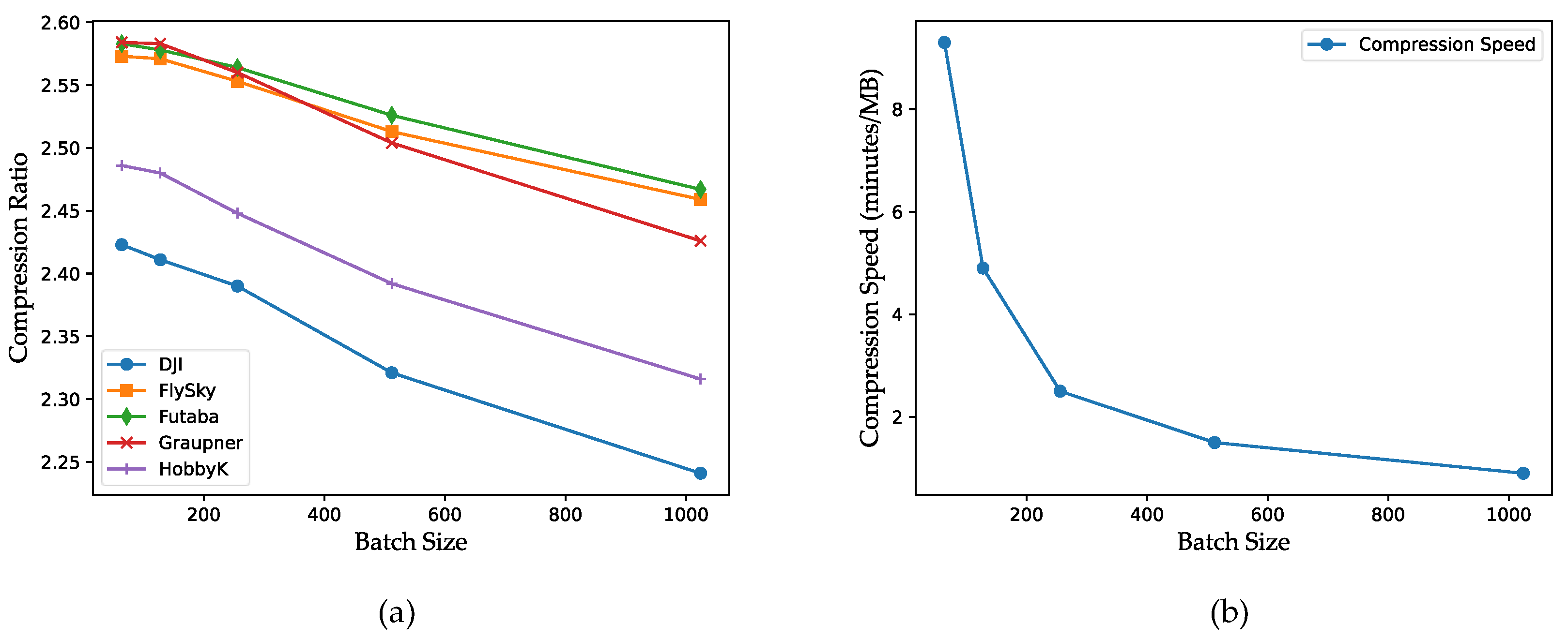
4.5. Compression Speed

In this sub-section, we compare the compression speed of MCDRC to CMIX. In our experiments, CMIX takes $13.6$ min/MB for compression on average, even with its highly optimized implementation. As for MCDRC, the compression speed is related to the batch size. The compression performance of MCDRC on the MPACT signals with different batch sizes (64, 128, 256, 512, and 1024) is reported in Figure 3. For each batch-size configuration, the experiment is repeated 10 times, and the median results are reported. Other hyper-parameters are the same as in Table 4.

As we can see from Figure 3, when the batch size increases, the compression ratio gradually decreases, but less time is needed for compression. Therefore, there is a trade-off between the compression ratio and the compression speed. When we use a batch size of 256, the proposed method consistently outperforms CMIX regarding the compression ratio and is five times faster. Note that this result also holds for decompression, since these two processes are symmetrical.

5. Conclusions

In this work, we present a context-based lossless compression technique using a novel recurrent neural network architecture, namely the MCRU, which is specially designed for compressing sensor signals. Experiments have proven that the BPC performance of the proposed MCRU on sensor datasets with more complex patterns outperforms classic recurrent units. Furthermore, MCRU is more robust to a sensor dataset with different ADC resolutions due to its flexible predictor resolution setting. Based on MCRU, we propose MCDRC, whose compression ratios on several datasets exceed the current state-of-the-art compressor CMIX. Regarding the running time of compression and decompression, although our work gives priority to the compression ratio, MCDRC achieves an obvious speed advantage over CMIX through a large batch size (256). The proposed MCDRC is five times faster than CMIX and can be further improved.

Many further ideas may be explored based on our work. For example, the highway operator $\mathcal{H}$ can be optimized to achieve stronger memory capability for the sensor signals. On the other hand, the channel number of MCRU can be set adaptively according to signal characteristics rather than pre-set to obtain better compression performance.

Although the proposed method has achieved state-of-the-art performance regarding the compression ratio on signal data, it is more suitable for offline compression due to its relatively slow compression speed. Therefore, another direction of future work can be implementing the proposed approach on hardware for real-time compression with low energy consumption.

References

1. Tan, L.; Yu, K.; Bashir, A.K.; Cheng, X.; Ming, F.; Zhao, L.; Zhou, X. Toward real-time and efficient cardiovascular monitoring for COVID-19 patients by 5G-enabled wearable medical devices: A deep learning approach. Neural Comput. Appl. 2021, 1–14. [Google Scholar] [CrossRef]
2. Manogaran, G.; Lopez, D. Disease surveillance system for big climate data processing and dengue transmission. In Climate Change and Environmental Concerns: Breakthroughs in Research and Practice; IGI Global: Hershey, PA, USA, 2018; pp. 427–446. [Google Scholar]
3. Lv, Z.; Hu, B.; Lv, H. Infrastructure monitoring and operation for smart cities based on IoT system. IEEE Trans. Ind. Inform. 2019, 16, 1957–1962. [Google Scholar] [CrossRef]
4. Qing, A.; Hongtao, Z.; Zhikun, H.; Zhiwen, C. A compression approach of power quality monitoring data based on two-dimension dct. In Proceedings of the 2011 Third International Conference on Measuring Technology and Mechatronics Automation, Shanghai, China, 6–7 January 2011; Volume 1, pp. 20–24. [Google Scholar]
5. Rui, Z.; Hong-jiao, Y.; Chuan-guang, Z. Compression method of power quality data based on wavelet transform. In Proceedings of the 2013 2nd International Conference on Measurement, Information and Control, Harbin, China, 16–18 August 2013; Volume 2, pp. 987–990. [Google Scholar]
6. Bruni, G.; Johansson, H.T. DPTC—An FPGA-Based Trace Compression. IEEE Trans. Circuits Syst. I Regul. Pap. 2019, 67, 189–197. [Google Scholar] [CrossRef] [Green Version]
7. Biagetti, G.; Crippa, P.; Falaschetti, L.; Mansour, A.; Turchetti, C. Energy and Performance Analysis of Lossless Compression Algorithms for Wireless EMG Sensors. Sensors 2021, 21, 5160. [Google Scholar] [CrossRef] [PubMed]
8. Shannon, C.E. A mathematical theory of communication. Bell Syst. Tech. J. 1948, 27, 379–423. [Google Scholar] [CrossRef] [Green Version]
9. Huffman, D.A. A method for the construction of minimum-redundancy codes. Proc. IRE 1952, 40, 1098–1101. [Google Scholar] [CrossRef]
10. Pasco, R.C. Source Coding Algorithms for Fast Data Compression. Ph.D. Thesis, Stanford University, Stanford, CA, USA, 1976. [Google Scholar]
11. Duda, J.; Tahboub, K.; Gadgil, N.J.; Delp, E.J. The use of asymmetric numeral systems as an accurate replacement for Huffman coding. In Proceedings of the 2015 Picture Coding Symposium (PCS), Cairns, QLD, Australia, 31 May–3 June 2015; pp. 65–69. [Google Scholar]
12. Ziv, J.; Lempel, A. A universal algorithm for sequential data compression. IEEE Trans. Inf. Theory 1977, 23, 337–343. [Google Scholar] [CrossRef] [Green Version]
13. Ziv, J.; Lempel, A. Compression of individual sequences via variable-rate coding. IEEE Trans. Inf. Theory 1978, 24, 530–536. [Google Scholar] [CrossRef] [Green Version]
14. Mahoney, M.V. Adaptive Weighing of Context Models for Lossless Data Compression; Technical Report; Florida Institute of Technology: Melbourne, FL, USA, 2005. [Google Scholar]
15. Knoll, B.; de Freitas, N. A machine learning perspective on predictive coding with PAQ8. In Proceedings of the 2012 Data Compression Conference, Snowbird, UT, USA, 10–12 April 2012; pp. 377–386. [Google Scholar]
16. Hochreiter, S.; Schmidhuber, J. Long short-term memory. Neural Comput. 1997, 9, 1735–1780. [Google Scholar] [CrossRef] [PubMed]
17. Goyal, M.; Tatwawadi, K.; Chandak, S.; Ochoa, I. DZip: Improved general-purpose loss less compression based on novel neural network modeling. In Proceedings of the 2021 Data Compression Conference (DCC), Snowbird, UT, USA, 23–26 March 2021; pp. 153–162. [Google Scholar]
18. Byron, K. Tensorflow-Compress. 2020. Available online: https://github.com/byronknoll/tensorflow-compress (accessed on June 2021).
19. Dai, S.; Liu, W.; Wang, Z.; Li, K.; Zhu, P.; Wang, P. An Efficient Lossless Compression Method for Periodic Signals Based on Adaptive Dictionary Predictive Coding. Appl. Sci. 2020, 10, 4918. [Google Scholar] [CrossRef]
20. Huang, F.; Qin, T.; Wang, L.; Wan, H.; Ren, J. An ECG signal prediction method based on ARIMA model and DWT. In Proceedings of the 2019 IEEE 4th Advanced Information Technology, Electronic and Automation Control Conference (IAEAC), Chengdu, China, 20–22 December 2019; Volume 1, pp. 1298–1304. [Google Scholar]
21. Graves, A. Generating Sequences with Recurrent Neural Networks. arXiv 2013, arXiv:1308.0850. [Google Scholar]
22. Hutter Prize. 2020. Available online: http://prize.hutter1.net/ (accessed on September 2021).
23. Silesia Open Source Compression Benchmark. 2021. Available online: http://mattmahoney.net/dc/silesia.html (accessed on September 2021).
24. Rumelhart, D.E.; Hinton, G.E.; Williams, R.J. Learning representations by back-propagating errors. Nature 1986, 323, 533–536. [Google Scholar] [CrossRef]
25. Luo, W.; Yu, F. Recurrent Highway Networks With Grouped Auxiliary Memory. IEEE Access 2019, 7, 182037–182049. [Google Scholar] [CrossRef]
26. Cho, K.; van Merrienboer, B.; Gulcehre, C.; Bahdanau, D.; Bougares, F.; Schwenk, H.; Bengio, Y. Learning Phrase Representations using RNN Encoder-Decoder for Statistical Machine Translation. arXiv 2014, arXiv:1406.1078. [Google Scholar]
27. Kriechbaumer, T.; Jacobsen, H.A. BLOND, a building-level office environment dataset of typical electrical appliances. Sci. Data 2018, 5, 180048. [Google Scholar] [CrossRef] [PubMed]
28. Piczak, K.J. ESC: Dataset for environmental sound classification. In Proceedings of the 23rd ACM International Conference on Multimedia, Brisbane, Australia, 26–30 October 2015; pp. 1015–1018. [Google Scholar]
29. Ezuma, M.; Erden, F.; Anjinappa, C.K.; Ozdemir, O.; Guvenc, I. Drone Remote Controller RF Signal Dataset; IEEE Dataport; IEEE: Piscataway, NJ, USA, 2020. [Google Scholar] [CrossRef]
30. Ilya, G. BSC. 2015. Available online: http://libbsc.com/ (accessed on June 2021).
31. NVIDIA. Framework-Determinism. 2019. Available online: https://github.com/NVIDIA/framework-determinism (accessed on June 2021).
Figure 1. Working flow of a context-based lossless compressor with a probability predictor and an entropy-coding module.
Applsci 11 10240 g001
Figure 2. Structure of the proposed multi-channel recurrent unit.
Applsci 11 10240 g002
Figure 3. The relationship between the batch size and (a) the compression ratio; (b) the average compression speed.
Applsci 11 10240 g003