An Enhanced Evolutionary Student Performance Prediction Model Using Whale Optimization Algorithm Boosted with Sine-Cosine Mechanism

Abstract

The students’ performance prediction (SPP) problem is a challenging problem that managers face at any institution. Collecting educational quantitative and qualitative data from many resources such as exam centers, virtual courses, e-learning educational systems, and other resources is not a simple task. Even after collecting data, we might face imbalanced data, missing data, biased data, and different data types such as strings, numbers, and letters. One of the most common challenges in this area is the large number of attributes (features). Determining the highly valuable features is needed to improve the overall students’ performance. This paper proposes an evolutionary-based SPP model utilizing an enhanced form of the Whale Optimization Algorithm (EWOA) as a wrapper feature selection to keep the most informative features and enhance the prediction quality. The proposed EWOA combines the Whale Optimization Algorithm (WOA) with Sine Cosine Algorithm (SCA) and Logistic Chaotic Map (LCM) to improve the overall performance of WOA. The SCA will empower the exploitation process inside WOA and minimize the probability of being stuck in local optima. The main idea is to enhance the worst half of the population in WOA using SCA. Besides, LCM strategy is employed to control the population diversity and improve the exploration process. As such, we handled the imbalanced data using the Adaptive Synthetic (ADASYN) sampling technique and converting WOA to binary variant employing transfer functions (TFs) that belong to different families (S-shaped and V-shaped). Two real educational datasets are used, and five different classifiers are employed: the Decision Trees (DT), k-Nearest Neighbors (k-NN), Naive Bayes (NB), Linear Discriminant Analysis (LDA), and LogitBoost (LB). The obtained results show that the LDA classifier is the most reliable classifier with both datasets. In addition, the proposed EWOA outperforms other methods in the literature as wrapper feature selection with selected transfer functions.

1. Introduction

Students’ performance prediction (SPP) problem is a common challenge for institutions’ lecturers and decision-makers to develop the best educational strategies for students. To perform such a prediction, several educational parameters can be employed to evaluate the performance of students, such as exams grades, Grade Point Average (GPA), lecture absenteeism, number of attempts to pass a course or an exam. Moreover, other demographic features such as gender, family relationship, parent profession, marital status, and personal habits [1,2]. Predicting students’ performance for educational organizations has been conducted by many scientific communities. Examining a vast amount of educational data and extract their impacts on students’ performances is closely related to educational data mining (EDM) and machine learning (ML) algorithms. Generally speaking, EDM is a set of data mining methods that tries to extract hidden and valuable information from educational data to expand our understanding of students’ performance and enhance the learning process [3,4].

EDM applications require two types of data: (i) educational data collected from educational systems such as exams centers, virtual courses, registration offices, and e-learning systems, and (ii) demographic data that presents information about students. Demographic data is usually collected by surveys or personal meetings. Both types of data can be used to build a robust EDM application, which is able to manipulate seemingly meaningless educational data into valuable knowledge that can improve the learning process and avoid negative performance [5]. In EDM, generally speaking, different kinds of data mining methods are needed, including but not limited to classifications [6], clustering [7], association rule mining [8], and web mining [9]. Moreover, due to modern learning technologies such as online classrooms, exams, and seminars, EDM applications can manipulate educational data accurately for a better understanding of the students’ performance, and learning process [10]. Such EDM applications can assist both tutors and decision-makers in executing suitable learning strategies that fit their students.

In reality, there are many advantages of EDM applications, such as revealing the weaknesses of the learning process between the teachers and students, predicting dropout potential, and negative student behaviors [11]. Moreover, it can determine the lapses and weaknesses of teaching strategies. EDM applications assist with reviewing the current learning models and evaluate their effectiveness. It can be used to evaluate the feedback information obtained from students and determine the limitations of the learning processes. EDM can cluster students based on their levels based on different criteria such as personal skills, learning behaviors, social attitudes, and interests [12].

EDM and ML allow us to design a learning model(s) to predict students’ performance as a classification or recognition model(s). However, selecting a robust ML model is a challenging task due to several factors such as data nature, imbalanced data, noisy data, incomplete data, and the number of collected samples. Imbalanced data plays a vital role that affects the overall performance of ML models. For example, the number of passed students is much higher than the number of failed students, and the performance of learning model(s) will be influenced toward passed students. So, the learning process will suffer from overfitting problem. As a result, it is essential to analyze the educational data before building the EDM application. Moreover, the educational data should not have missing data to prevent the unstable behavior of the ML model. Several research papers addressed the imbalanced educational datasets while building ML models [13,14,15]. In general, imbalanced data is manipulated based on data level (e.g., resampling methods) or algorithm level (e.g., cost-sensitive learning). 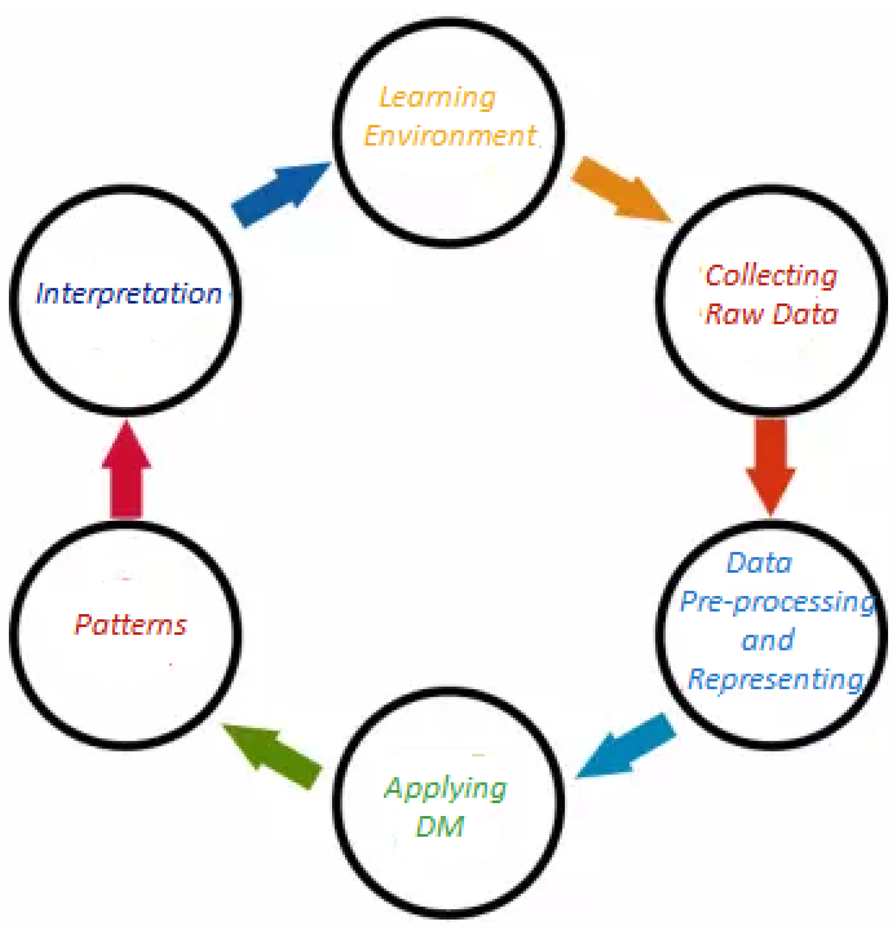Figure 1 depicts the life cycle of EDM process.

In data mining techniques (e.g., classification), data preprocessing has a major impact on both the quality of chosen features and the performance of learning algorithms [16,17]. Feature selection (FS) is a fundamental preprocessing stage that aims to uncover and keep informative patterns (features) and remove noisy, uninformative, and irrelevant ones from the feature space. Detecting high-quality subset of features will boost the accuracy of learning classifiers and lessen the computational cost [18,19]. According to assessment criteria of the selected subset of features, FS techniques follow one of two branches: filters or wrappers [19,20]. Filter FS methods utilize scoring matrices for estimating the excellence of the selected subset of features. In other words, in filter type, features are weighted using a filter technique (e.g., information gain or chi-square), and then the features that possess weights less than a pre-set threshold are excluded from the features set. In the case of wrapper FS, a learning classifier (e.g., Linear Discriminant Analysis or K-Nearest Neighbour) is hired to decide the excellence of subsets of features produced by a search approach [21,22]. In general, in comparison with filter methods, wrapper FS can deliver better performance because it can implicitly discover and employ dependencies between features of a subset, whereas filter FS may miss such an advantage. However, the computational cost of using filter FS is cheaper than wrapper FS [23].

Feature subset generation is identified as a search operation for finding a high-quality subset from a given set of patterns where a search mechanism such as complete/exact, random, or a heuristic is employed [24,25,26]. In a complete search, all potentially obtainable feature subsets in the search space are formed and assessed. In other words, if a dataset includes M features, then $2^M$ subsets will be obtained and examined to identify the most valuable one. Complete search is impractical when dealing with massive datasets because of its high computational cost. Random search is another mechanism for generating subsets of features. In this mechanism, looking for the following feature subset in the feature space is done randomly [27]. In some cases, the random search may lead to generate all potential subsets of features as in the complete search mechanism [18,28]. Compared to complete and random search, heuristic search is a different search mechanism for generating subsets of features. It is defined by Talbi [28] as upper layer general methods that can be employed as guiding mechanisms to design underlying heuristics for resolving particular optimization problems. In contrast to complete/exact methods [29,30], meta-heuristics algorithms such as Particle Swarm Optimization (PSO) and Ant Colony Optimization (ACO) have demonstrated outstanding ability in solving many FS problems [19,31,32,33].

WOA is a modern meta-heuristic algorithm, introduced by Mirjalili and Lewis [34]. It simulates the humpback whales’ intelligent foraging behavior. WOA possesses a simple structure that makes it easy to implement. It also has only two primary parameters that need to be adjusted. In addition, the WOA algorithm depends on just one parameter for smooth shifting from exploration to exploitation. WOA has shown high exploration ability. Unlike other meta-heuristic algorithms, WOA updates the position vector of a whale (solution) in the exploration stage with respect to the position vector of a randomly chosen search agent rather than the optimal search agent discovered so far [17,34,35,36]. Like other meta-heuristic algorithms, WOA has drawbacks like early convergence and the ease of falling into the local optimum. Hence, scholars have made several improvements to the basic version of WOA to overcome its limitation and employed it to solve various optimization problems. For instance, [35] proposed an improved version of WOA based on Natural Selection Operators and applied it as a wrapper feature selection method for software fault prediction. Mafarja and Mirjalili [17] combined WOA with simulated annealing (SA) algorithm to enhance its exploitation ability and applied their enhanced WOA-based approach for feature selection. Also, Ning and Cao [36] proposed an improved variant of WOA and applied it for solving complex constrained optimization problems. A Mixed-Strategy-based WOA was proposed by Ding et al. [37] for optimizing the parameter of a hydraulic turbine governing system (HTGS). Abdel-Basset et al. [38] proposed Levy flight and logical chaos mapping based WOA approach and employed it to tackle virtual machine (VM) placement problem. As presented in [39], WOA has the same problem as many other optimization algorithms and tends to be stuck into local optima. To overcome this problem, two enhancements for the WOA algorithm were proposed. The first improvement involves applying Elite Opposition-Based Learning (EOBL) the initialization stage of WOA, whereas the second one includes the integration of evolutionary operators comprising mutation, crossover, and selection from the Differential Evolution algorithm at the end of every WOA iteration. Since the WOA-based algorithms have been widely and effectively used in various applications, this is the foundation and motivation of this research as well.

This paper proposes an evolutionary-based SPP model that integrates an enhanced variant of WOA (EWOA) with an ML algorithm. The new variant EWOA is used to enhance the FS process and the prediction of students’ performance. The efficiency of the proposed model developed in this research is evaluated on two real, imbalanced, and public educational datasets adopted from the literature. To sum up, the main contributions of this research are as follows:

• The ADASYN sampling technique is applied to handle the problem of imbalanced data.
• Various types of well-known ML algorithms are assessed to select the best-performing one to handle the SPP problem.
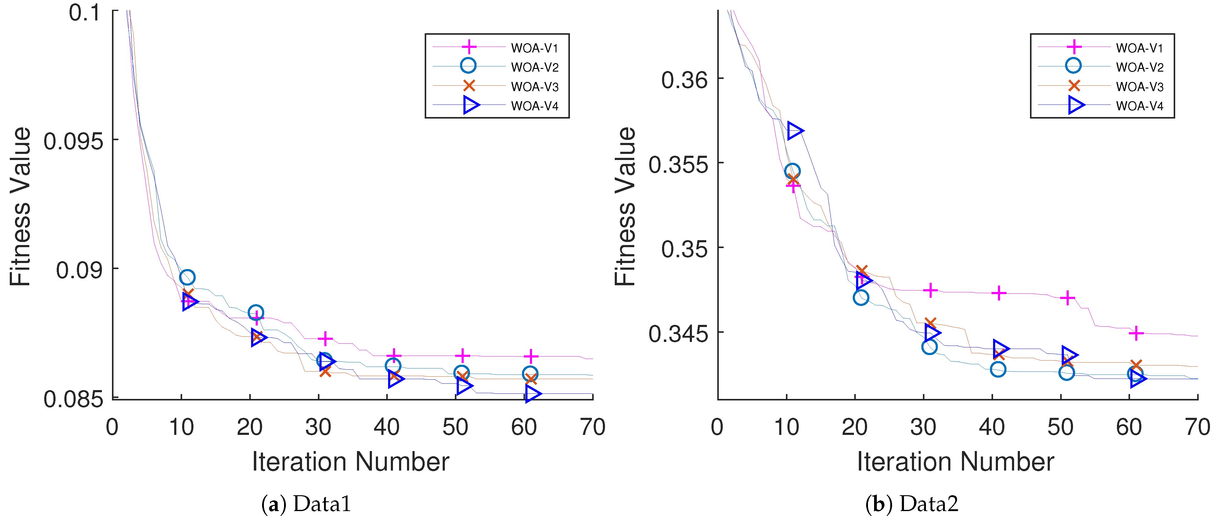
• Eight fuzzy transfer functions from S-shaped and V-shaped families are examined to prepare WOA to match the binary search space of the FS problem.
• An improved form of the WOA algorithm is introduced by combining it with the Sine Cosine Algorithm (SCA) and Logistic Chaotic Map (LCM) mechanism. The main objectives are overcoming the main weak point of WOA (i.e., weakness exploitation process) and keeping an appropriate scale between exploration and exploitation processes.
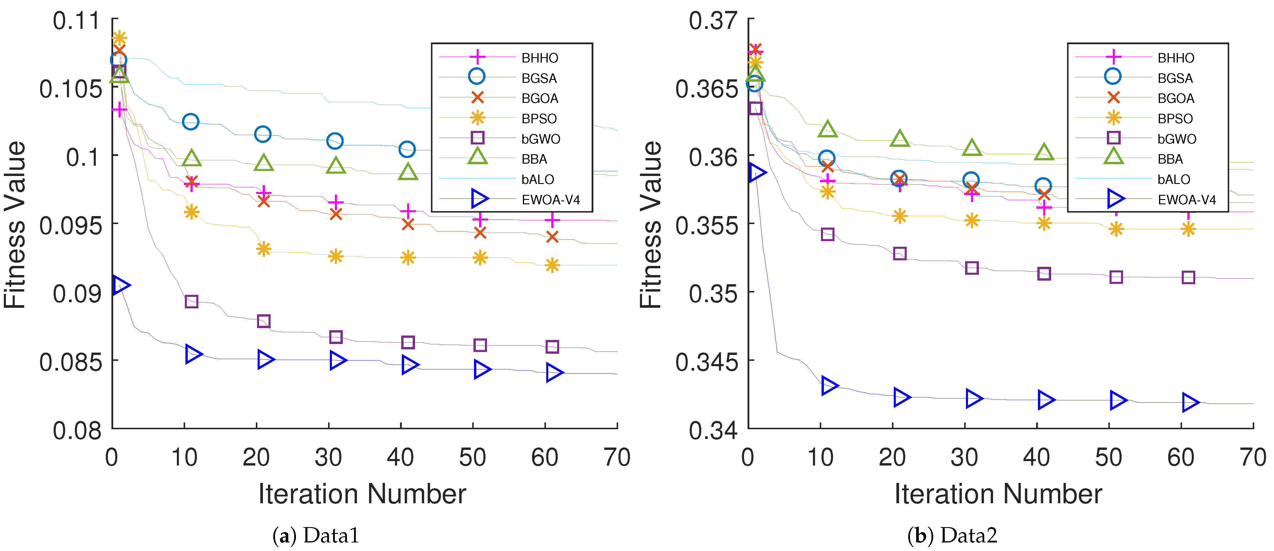
• The performance of the proposed EWOA is evaluated against the state-of-the-art metaheuristic algorithms and shows promising results.

The rest of the paper is organized as follows: Section 2 presents the related works of SPP and related EDM applications. Section 3 explores the proposed methods. Section 4 explores the educational datasets used in this work. Section 5 presents the performance evaluation criteria for the proposed method. The results and analysis are presented in Section 6. Finally, the conclusion and future works are presented in Section 7.

2. Related Work

The principle of EDM has gained the interest of scholars due to its hardness and significance to the educational field. Data mining algorithms have been employed in different manners for addressing the EDM problem depending on the nature of the problem, such as classification, clustering, and sequential pattern analysis [40,41]. In addition to the aforementioned classes, some hybrid approaches that benefit from more than one technique (e.g., classification and clustering) were proposed for improving the prediction of the performance of students [42,43]. Recently, researchers also employed wrapper FS approaches that combine ML classifiers and optimization algorithms to improve the overall performance of SPP models [15,44]. The following subsections explore related works for each category.

2.1. Classification Methods

Classification techniques such as; Decision Trees (DT), Support Vector Machines (SVM), Naive Bayes (NB), and Artificial Neural Networks (ANN) are widely used in the field of education to predict students’ performance. For example, as stated in [45], the DT classifier was applied to predict the final grades of students in a university course under study. Ahmad et al. [46] used eight-year data from 2006 to 2014 of undergraduate students to predict their academic performance in computer science courses. The applied dataset contains information such as gender, hometown, family income, and GPA. In addition, three classification algorithms comprising DT, Rule-Based (RB), and NB were utilized for building SPP models. The experimental results revealed that the RB classifier is the best one compared to the other classifiers by recording the highest accuracy rate of 71.3%. Hamsa et al. [47] proposed an academic performance prediction model using two approaches, including fuzzy genetic algorithm (FGA) and DT. Internal and sessional makes along with admission scores were selected as features. The resultant prediction model can be used to determine the students’ performance for each module. Hence, instructors can identify low-performing students and take early steps to improve their performance.

SVM has been applied in SPP fields. For instance, Asogbon et al. [48] tried to accurately predict students’ performance with the aim of place them into suitable faculty courses where a multi-class SVM (MSVM) classifier was used to build the prediction model. In addition, the educational students’ dataset from the University of Lagos, Nigeria, was applied to examine the proposed model. Findings of the experiments revealed that MSVM based SPP model with 7-fold cross-validation could correctly predict students’ performances and provide the university management with the required information for placing students in various academic programs. In addition, Pratiyush and Manu [49] utilized an SVM classifier for predicting the placement of students. The proposed model was evaluated on an educational dataset of students containing six features: attendance, GPA, reasoning, quantitative, communication skills, and technical skills. The authors stated that prediction results could provide educational institutions a better understanding of how students should be placed. Furthermore, based on the psychological information (features) of students, Burman and Som [50] proposed a classification model using SVM to categorize students into three classes, including high, average, and low, depending on their academic performance. Experimental results showed that SVM with Radial Basis kernel function could provide better accuracy than using Linear Kernel function, which is nearly 90%. Another example of using classification approaches in the field of education for predicting the performance of students can be found in [51]. In this study, two classifiers, NB and SVM, were applied over students’ data such as residence, GPA, and profile data to predict whether their college student will finish their studies in four years or less. Experimental results showed that SVM surpassed NB with $69.15\%$ accuracy.

Using the NB classifier in the field of SPP, Shaziya et al. [52] introduced a model for predicting students’ performance in semester exams. This model is based on NB classifier and is used to predict the end-of-semester results of students. The outcome of the proposed model can help students in improving their academic performance. Makhtar et al. [53] estimated student’s performance using NB classifier. The proposed model is utilized to discover the hidden patterns between subjects that influence the performance of students. In addition, the Best-First approach was applied for feature selection. Results have shown the superiority of the NB algorithm in predicting the performance of students compared to several classifiers such as Random TreeMulti-Classes Classifier, Conjunctive Rule, Nearest Neighbour, and Lazy IB1. The authors concluded that the NB classifier could be utilized for the classification of students’ performance in the early phase of the second semester with 74% accuracy.

Neural network (NN) classifier is also utilized to develop automated SPP models. As presented in [54], for instance, the authors used Back Propagation Neural Network (BP-NN) based on the classification to predict future student performance based on their previous knowledge along with other new students with similar characteristics. Academic data of six subjects for 60 high school students were used for model evaluation. Results show that the model is able to produce precise results. Rana and Garg [55] also applied two machine learning classifiers, including NN and NB, using WEKA machine learning software to predict the performance of students. The authors evaluated the proposed models on a small dataset that includes information of 58 students. The recorded results confirmed that NB is better than the NN classifier.

As stated earlier, FS is a core pre-processing procedure that aims to find and eliminate noisy, uninformative, and irrelevant features from datasets to reduce data dimensionality and boost the efficiency of machine learning classifiers. Wrapper and filter-based FS approaches have been applied for some works in the area of SPP. For example, in [56], a filter FS approach based on information gain (IG) was employed to filter the highly informative students’ behavioral features for building prediction models. A set of ML classifiers including DT, ANN, and NB boosted with ensemble methods such as bagging and boosting were utilized for classification. Results showed that using students’ behavioral features can remarkably enhance the performance of students’ prediction model. In [14], a feed-forward Multi-Layer Perceptron (MLP) technique integrated with stochastic training algorithms was applied as an SPP model. In addition, IG was exploited as an FS approach, and the SMOTE oversampling technique was applied to deal with the problem of imbalanced data. Experimental results confirmed that the proposed MLP based approach efficiently resolves SPP problems compared with several ML classifiers such as DT, KNN, Logistic Regression (LR), Linear Discriminant Analysis (LDA), SVM, and Random Forest (RF), plus a set of state-of-the-art methods.

Wrapper FS approaches that combine optimization algorithms with ML classifiers have also been applied to improve the performance of SPP models. For instance, a wrapper-based FS technique was proposed by Turabieh et al. [44] for resolving the problem of SPP. In this technique, an improved form of the recent Harris Hawks Optimization algorithm (HHO) was applied to explore the search space for discovering the most informative features. In addition, the KNN classifier was used for evaluating the goodness of the produced subsets of features by the HHO algorithm. Several ML classifiers, including KNN, Layered recurrent neural network (LRNN), NB, and ANN, were applied over a real student performance prediction dataset to assess the overall performance of the SPP system. Most Promising accuracy value was achieved when HHO is applied in conjunction with the LRNN classifier, which is equal to 92%. Another wrapper FS approach based on Binary Teaching-Learning Based Optimization (TLBO) was introduced by Alraddadi et al. [15] for improving the performance of student performance prediction. TLBO algorithm was applied as a search strategy while various ML classifiers (i.e., SVM, LDA, LR, RF, and DT) were used for evaluating the quality of subsets of features generated by the TLBO algorithm. Moreover, two real student performance prediction datasets were adopted for evaluation purposes. It was observed that the utilized datasets are highly imbalanced. For this reason, oversampling techniques (i.e., SMOTE) were applied over the datasets to handle the problem of imbalanced data. The experimental results proved the power of the proposed wrapper FS in improving the classification performance of LR and LDA classifiers. TLBO algorithm demonstrated its capability to improve the overall performance of ML classifiers. The AUC results of TLBO with LDA classifier are increased up to 3% and 8% for both examined datasets compared with the results of LDA without applying the feature selection approach (TLBO).

2.2. Clustering Methods

Clustering is known as an unsupervised ML technique where data are classified into clusters of data that have similar characteristics that are different than the characteristics of the data in the other clusters [57]. Various clustering algorithms were applied to educational datasets to cluster students based on their performance in order to give educational organizations better insights in understanding their students and their different learning styles to find the best strategies for their students’ success [58]. For example, in [59] Harwati et al. employed the k-mean clustering method to classify their student performance to improve it. Their study was carried on using data for 306 students from different universities. The collected data consist of demographic features such as gender, origin, GPA, grade of certain courses, and course attendance. They found that these input features formed three different clusters; smart, normal, and low. Park et al. [60] employed the latent class analysis (LCA) method as a clustering method for educational data to extract common features from online behavior data of 612 courses tracked from the Learning management system and database of a South Korean University. Their work identified four different clusters of how Blended Learning is adopted and implemented, which gives the educational organization better visualization of the data and helps in providing strategic plans. These groups are immature which consist of 50% of the courses, collaboration (24.3%), discussion (18%) and sharing (7.2%). Valsamidis et al. [61] proposed a methodology based on two clustering algorithms; Simple K-means and Markov Clustering (MCL) for the purpose of improving the content quality of Learning Management Systems (LMS) by analyzing their log data files. The former algorithm is used to cluster the courses and the latter for clustering the students’ activity, giving the instructors better insights into both students and courses.

2.3. Sequential Pattern Analysis Methods

Sequential pattern analysis methods are used to discover hidden knowledge by finding the unknown interrelationships and data patterns [62]. Many research papers investigated EDM using sequential pattern analysis methods. Simpson et al. [63] investigated eEDM for classrooms using sequential pattern analysis methods to discover severe expressive communication in the environment of general education. Nakamura et al. [64] proposed a sequential pattern analysis method to extract good knowledge from learning histories of programming courses. The authors developed a tool for collecting learning histories. The proposed approach offers an excellent analysis of the relationships between learning situations and learning processes in programming courses.

2.4. Hybrid Methods

Hybrid methods are a branch of data mining that combines multiple existing data mining techniques to enhance the methods’ performance and results. In [42], a hybrid approach was proposed by combining clustering and sequential patterns methods to improve student performance. The authors tested their methods on a real dataset, and the results were promising. Tarus et al. [65] employed a hybrid approach between ontology and sequential pattern mining to discover hidden knowledge for real data obtained from a public university. The proposed method shows excellent results for decision-makers. In [43], students’ information, including various features such as demographic, academic, behavior, and others, were collected and used to construct students’ performance prediction model in which classification and clustering techniques were applied. Four classifiers, including SVM, NB, DT, and NN, were utilized to assess the students’ performance dataset measures. Based on the results of classification, the optimal features that provide best results were identified. Then, K-Means clustering in conjunction with the majority vote method was applied to predict students’ academic performance. The accuracy of the hybrid SPP model that combines clustering and classification is 0.7547% when used with academic, behavior, and other features of the students’ performance dataset. The proposed SPP model confirmed its superiority compared to other existing models.

In addition to the categories mentioned above, fuzzy logic has also been applied to predict students’ performance. For instance, Rojas et al. [66] proposed a fuzzy logic-based model that enables educational institutions and teachers to monitor the process of the academic performance of students continuously. Lee et al. [67] proposed a fuzzy evaluation model for e-learning using importance and satisfaction measures where a performance evaluation matrix was used. A fuzzy evaluation model based on fuzzy linguistic hedges for students’ academic progress was proposed by [68]. The model modifies the grades of questions by integrating factors such as complexity, importance, and difficulty of examination questions to reflect skills and deep learning obtained through the course.

Finally, we can conclude that examining educational data to improve the overall educational process is needed. Since educational data is high dimensional, ML methods are most suitable to analyze and find hidden knowledge. To achieve this, we believe that employing wrapper FS methods will help educational organizations to understand the most valuable factors (i.e., features) that affect the student’s performance. Therefore, in the next section, we propose an enhanced wrapper FS method based on WOA.

3. Proposed Approach

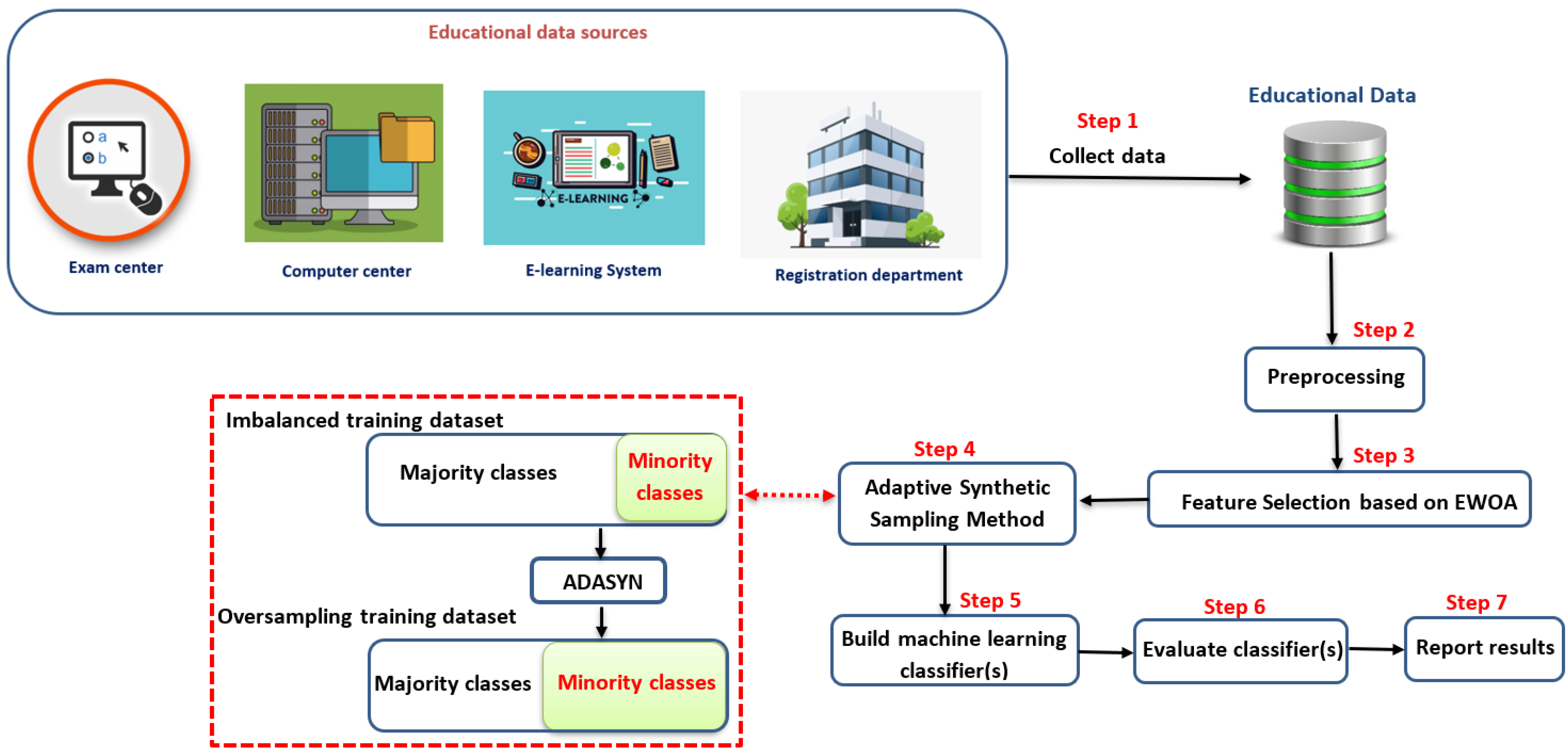
The proposed approach is depicted in Figure 2. The proposed approach has seven steps as follows:

• Collecting data from different educational resources, where this data may have different data types such as numbers (i.e., grades), letters (i.e., gender), strings (i.e., major, address, course names, etc.).
• Preprocessing the collected data in order to be consistent. In this step, we removed all the records that have missing attributes and normalized the data between [0,1].
• Apply EWAO as a feature selection to reduce the search space and remove the weakness attributes that have no impact on the overall performance.
• Apply an ADASYN to overcome the imbalanced data and avoid overfitting problem while learning process.
• Build a machine learning classifier that is able to predict the students’ performance.
• Evaluate the obtained results based on the area under the ROC curve (AUC).
• Finally, the obtained results are reported.

The following subsections explore the main methods employed in the proposed methodology. First, an overview of the ADASYN oversampling technique is presented in Section 3.1. Second, an overview of the basic WOA is presented in Section 3.2. Third, the main components of our enhancement over WOA are presented in Section 3.3 and Section 3.4, respectively. The Logistic Chaotic Map (LCM) is presented in subSection 3.3, where LCM is proposed inside the WOA to control the population diversity. The updating mechanism of the proposed enhancement is performed based on SCA, which is presented in Section 3.4. The proposed EWOA is presented in Section 3.5, which combines WOA, LCM, and SCA as a new FS algorithm. Section 3.6 explains how transfer functions are used to convert the original WOA to match the binary search space for the FS problem. Finally, Section 3.7 presents the formulation of FS as an optimization problem (i.e., fitness function and solution encoding).

3.1. ADASYN for Handling Imbalanced Data

Learning from imbalanced data is a significant challenge that could degrade the prediction quality of ML algorithms. This problem appears in most real classification problems where the target classes are not approximately equally represented [69]. For instance, in binary classification problems, the data samples of one class are normally limited (rare instances) compared to other samples. In such situations, the classification algorithm is trained using highly imbalanced data. Thus, it tends to choose the patterns in the majority classes, which results in imprecise minority class prediction [70].

ADASYN is a promising synthetic sampling approach developed basically over the idea of SMOTE approach, which both have been extensively employed to handle the problem of imbalanced learning [71]. The main concept of ADASYN is to generate minority data samples considering their distributions adaptively. In specific, more synthetic data is produced for the samples of minority class that are difficult to learn in contrast with minority class samples that are simpler to learn. ADASYN facilitates learning from imbalanced data by achieving two objectives; it reduces the learning bias towards the dominant class and adapts the decision boundary to focus on those more challenging to learn samples. The detailed procedure of ADASYN can be found in [71].

3.2. Whale Optimization Algorithm

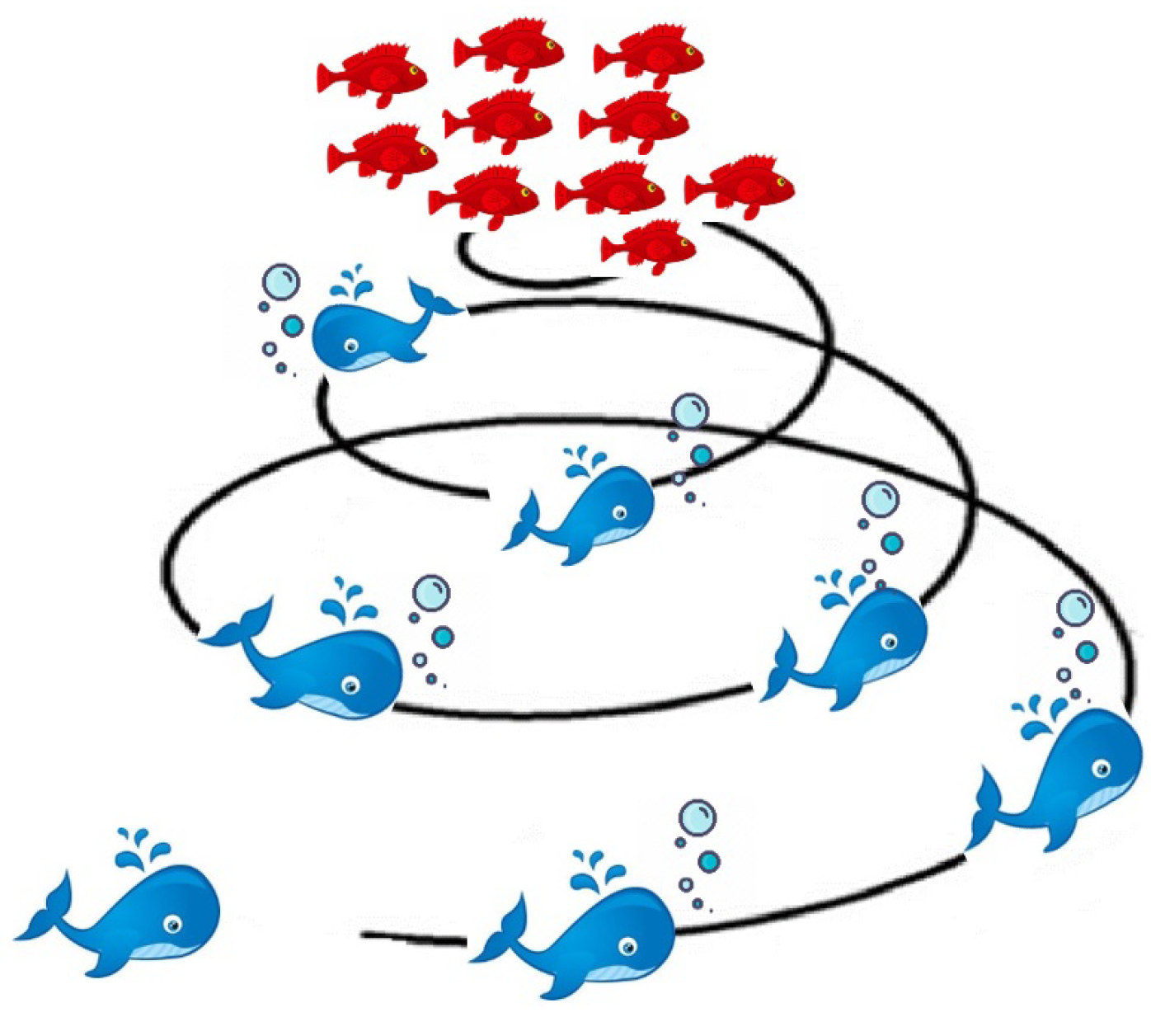
Whales are considered the largest mammals that live in groups. Among the types of whales is the humpback whale [34]. In nature, Humpback whales have a wonderful hunting strategy to find food such as krill and fishes [72]. The search strategy for humpback is named bubble-net feeding, in which humpback creates bubbles in an upward spiral swimming track around the target (i.e., fish, seals, squid, etc.) WOA is a swarm optimization method that simulates the process of the humpback whales while searching for their foods in the oceans based on creating bubble-nets to constrict the prey, and then whales move toward their preys in a spiral shape before the attack. Mirjalili and Lewis [34] proposed WOA in 2016, which mimics the searching process for whales while hunting. The exploration process inside WOA simulates the encircling mechanism of the whales in nature. The authors represent the prey location as the best solution found so far, while the rest solutions represent the candidate whales. Figure 3 demonstrates the spiral movement of the whale while searching for food. Since WOA is a population-based algorithm, the first phase of WOA is to create the initial population (humpback whales), as shown in the following Algorithm 1.

Algorithm 1 First phase of WOA algorithm.

Create initial population of whales(LB, UB, nopop, n) $LB$ = [$L{B}_1$, $L{B}_2$,..., $L{B}_n$] $UB$ = [$U{B}_1$, $U{B}_2$,..., $U{B}_n$] for j=1:nopop do     for m=1:n do         initial population(j,m)=($UB(m)-LB(m)$) × rand + $LB(m)$

where $LB$ presents lower bound of the decision variables, $UB$ presents the upper bound of the decision variables, $nopop$ presents the size of population, and n denotes number of decision variables.

3.2.1. Encircling Prey

The second phase of the WOA is to determine the best solution (whale) based on the fitness function. Each solution is structured as a vector of the decision variables. The rest solutions will update their positions in the search space with respect to the best solution using Equations (1) and (2).

$$\overrightarrow{D}=\mid \overrightarrow{C}·{\overrightarrow{X}}^{*}(k)-{\overrightarrow{X}}^{}(k)\mid$$

(1)

$${\overrightarrow{X}}^{}(k+1)={\overrightarrow{X}}^{*}(k)-{\overrightarrow{A}}^{}·\overrightarrow{D}$$

(2)

where k presents the current iteration, ${\overrightarrow{X}}^{*}$ presents the best solution so far, and $\overrightarrow{A}$ and $\overrightarrow{C}$ denote specific coefficient vectors estimated based on Equations (3) and (4), respectively. $\mid \mid$ denotes the absolute value, and · is a component-by-component multiplication. Note that the dimension of vectors is equal to the number of variables (features) of the problem being solved.

$$\overrightarrow{A}=2\overrightarrow{a}·\overrightarrow{r}-\overrightarrow{a}$$

(3)

$$\overrightarrow{C}=2·\overrightarrow{r}$$

(4)

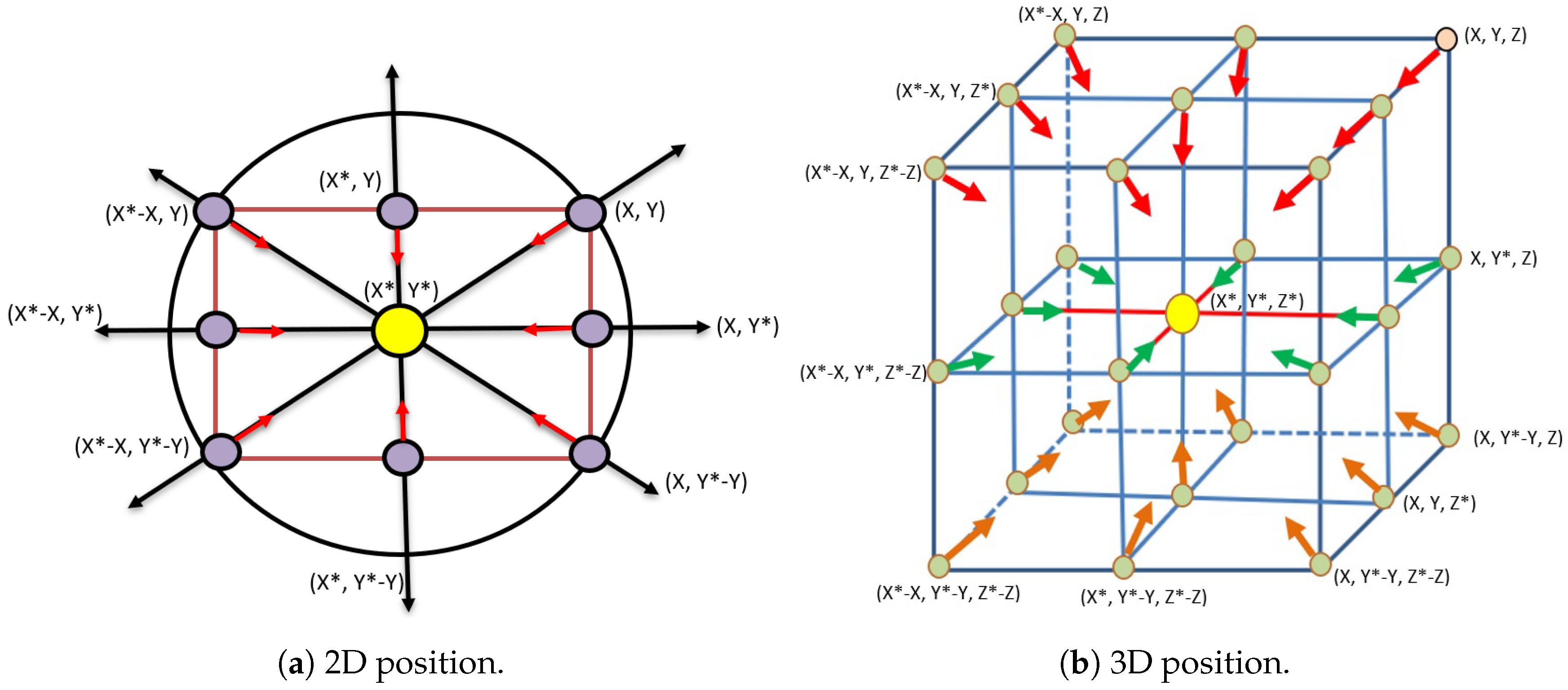
where $\overrightarrow{a}$ presents a variable with initial value equals 2. This variable will linearly decrease toward 0 after a set of iterations as in Equation (5). $\overrightarrow{r}$ is a random vector between 0 and 1, which is produced using a uniform distribution. Equations (1) and (2) give the WOA the ability to search in n-dimensional solution space (i.e., 2D and 3D) in an efficient manner as shown in Figure 4.

$$\overrightarrow{a}=2(1-\frac{k}{K})$$

(5)

where k is the current iteration, while K is the maximum number of iterations.

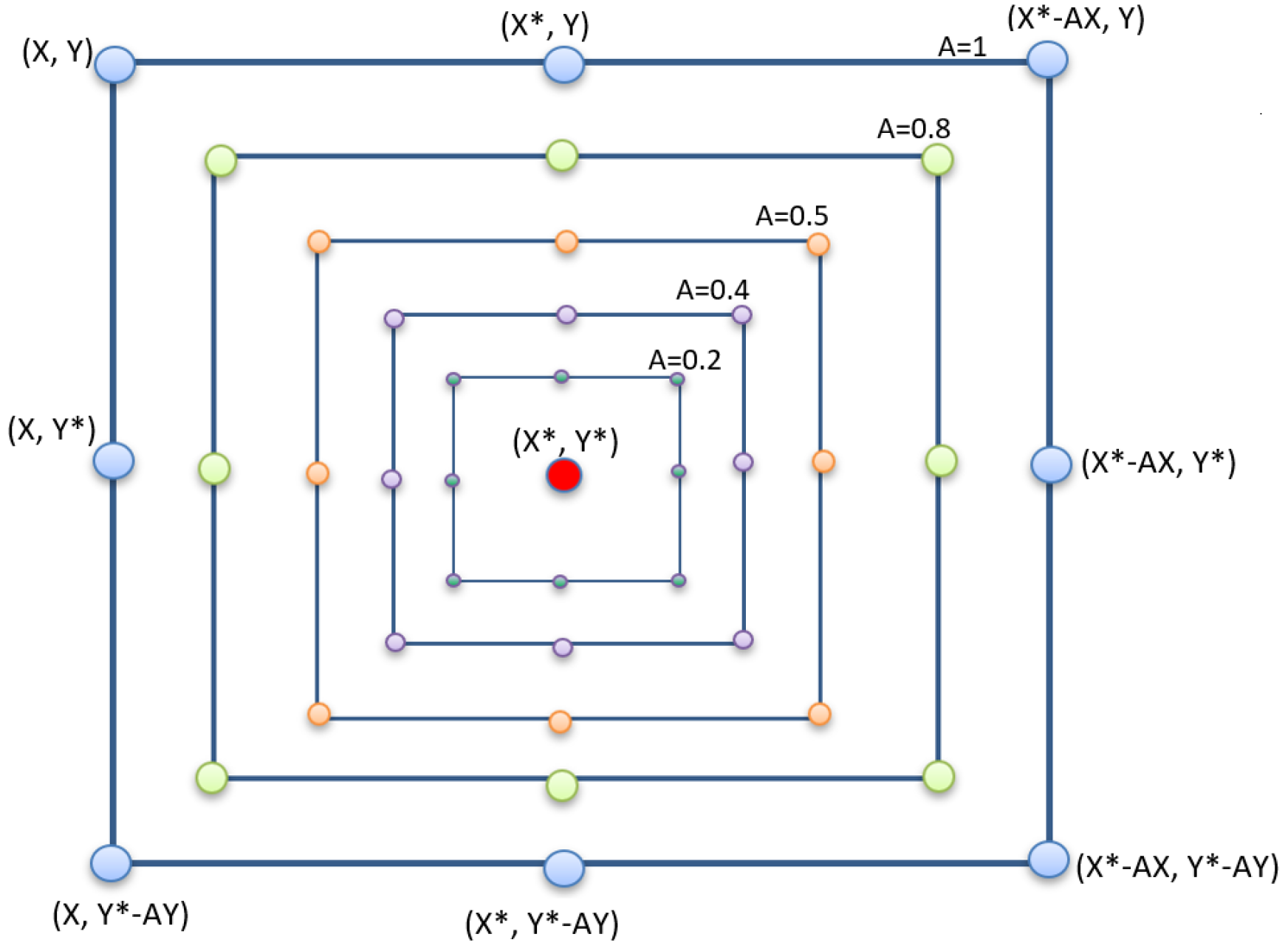
3.2.2. Bubble-Net Attacking

Two mathematical models have been proposed to mimic the whale performance while attacking their prays: The shrinking encircling mechanism and Spiral updating position. To update the whales’ position around the best solution in the search space, the shrinking encircling mechanism mimics this process by reducing the value of variable $\overrightarrow{a}$ over the course of generations in a linear manner. Figure 5 demonstrates the expected positions of whales around the best solution.

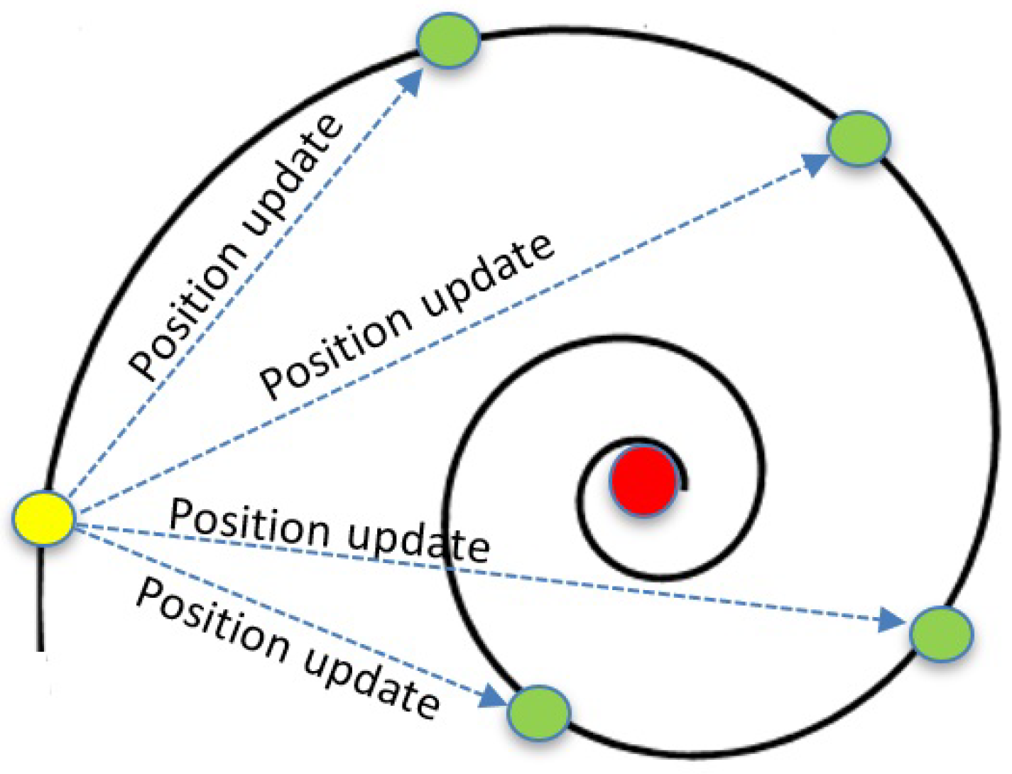
In nature, whales swim in an upward spiral path while hunting their food. To mimic this process, a logarithmic spiral function is used, as shown in Equation (6).

$$\overrightarrow{X}(k+1)={\overrightarrow{D}}^{\prime }·e^{bl}·cos(2\pi I)+{\overrightarrow{X}}^{*}(k)$$

(6)

where ${\overrightarrow{D}}^{\prime }=\mid \overrightarrow{x^{*}}(k)-\overrightarrow{X}(k)\mid$ denotes the distance between the ith solution and the optimal solution found so far, the parameter b creates the shape of the spiral function and I is random number between $-1$ and 1. Figure 6 depicts the spiral swimming process for whales while hunting.

To model the shrinking encircling and spiral swimming behaviors, a probability of $50\%$ is assumed to select between these two behaviors throughout the course of optimization. Each whale selects the operation to be performed randomly based on its location with respect to the optimal solution so far. Equation (7) explores the operation selection based on a random number p.

$$\overrightarrow{X}(k+1)=\left\{\begin{array}{cc}{\overrightarrow{X}}^{*}(k)-\overrightarrow{A}·\overrightarrow{D}\hfill & ,p<0.5\hfill \\ {\overrightarrow{D}}^{\prime }·e^{bt}·cos(2\pi I)+{\overrightarrow{X}}^{*}(k)\hfill & ,p\ge 0.5\hfill \end{array}\right.$$

(7)

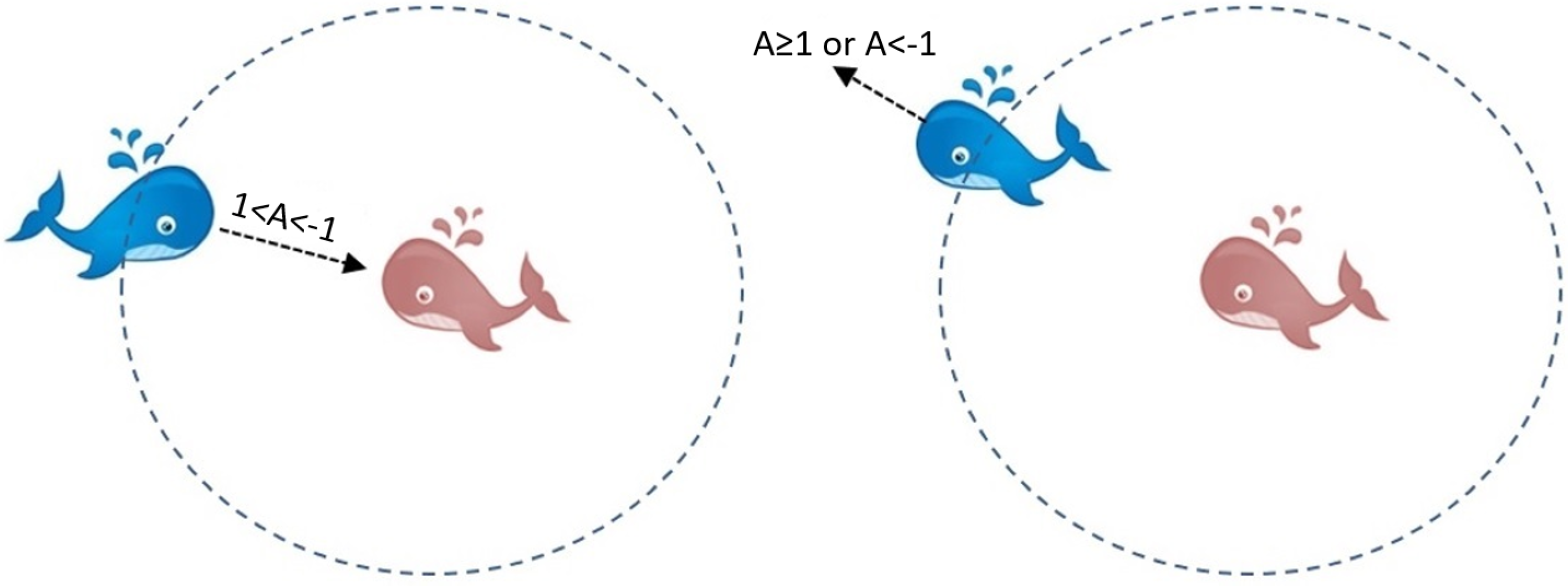
In simple, the exploration phase in WAO occurs once each whale in the population updates its position based on an arbitrarily selected whale. The next position for the whale will be in the area between its current position and the position of a randomly selected. The exploration phase occurs when the variable (A) has a value between −1 and 1 as shown in Figure 7. The exploitation phase occurs when each whale updates its current position based on the position of the best whale so far, where a linear decreeing of the variable (A). In simple, Equations (8) and (9) present the exploration phase of WOA. Finally, the Pseudo-code of WOA is presented in Algorithm 2.

$$\overrightarrow{D}=|\overrightarrow{C}·{\overrightarrow{X}}_{rand}-\overrightarrow{X}(k)|$$

(8)

$$\overrightarrow{X}(k+1)={\overrightarrow{X}}_{rand}(k)-\overrightarrow{A}·\overrightarrow{D}$$

(9)

Algorithm 2 Pseudo-code of WOA.

Initialize a random population of whales Initialize all coefficients Evaluate all solutions using fitness function Determine the optimal solution so far (denoted as $X^{*}$) while (k < maximum number of iterations) do     for each solution (whale) do         Update a, A, C, l, and p coefficients.         if (p < 0.5) then            if $|A|<1$ then                Update the current solution’s position by Eq.(2).            else if $|A|\ge 1$ then                Pick a random solution from the population                Update the position of $X(k)$ using Eq.(9)         else if (p≥ 0.5) then            Update the position of $X(k)$ by Eq.(6)     Estimate the fitness value for each in the population.     Update $X^{*}$     $k=k+1$ return$X^{*}$

3.3. Logistic Chaotic Map (LCM)

To improve the population diversity and increase the exploratory behaviour of WOA, a logistic chaotic map strategy is employed in this work. The chaotic map strategy is an efficient method to adjust parameter values to improve the exploration process and final solution. Moreover, the chaotic map strategy enhances the convergence speed and the search precision [73,74]. A chaotic sequence number is introduced to replace a random number in WAO algorithm (called p in WOA). The Equation (10) generates a logistic chaotic sequence number.

$$C_{t+1}=4·C_t·(1-C_t)$$

(10)

where $C_t$ is a chaotic sequence at iteration t. The initial value for $C_1$ is usually $0.8$, and the value interval is within [0,1]. The chaotic sequence number is employed to balance between two updating mechanisms (i.e., spiral-path and shrinking-circles path) inside the WOA. As a result, a logistic chaotic map will guarantee that $50\%$ of the iterations will go for each updating mechanisms.

Chaotic maps are frequently used to improve the performance of optimization algorithms. They are essentially utilized to enhance the convergence behaviors of meta-heuristic optimization algorithms and avoid being stuck into local optima. Chaotic maps are employed in meta-heuristic algorithms to produce chaotic variables instead of random ones. Chaos is a non-linear approach that has deterministic dynamic manners [74,75]. It is highly sensitive to its initial state where a large number of sequences can be simply produced by adjusting its initial state [74,75]. In addition, chaos has the characteristic of ergodicity and non-repetition. Hence, it can accomplish straightforward and faster searches in contrast with the stochastic searches that basically depend on probability distributions [76]. Chaotic maps have been used to promote the performance of many optimization algorithms such as particle swarm optimization (PSO) [74,77], Artificial bee colony (ABC) [75], Krill Herd optimization algorithm (KH) [76] and Bat Algorithm (BA) [78].

3.4. Sine-Cosine Algorithm

Sine-Cosine algorithm (SCA) is a population-based optimization algorithm that was introduced by Mirjalili in 2016 [79]. The main idea of SCA is that each solution will update its position with respect to the position of the best solution in the search space using Equations (11) and (12).

$$X_i^{k+1}=X_i^k+r_1\times sin(r_2)\times |r_3{P}_i^k-X_i^k|$$

(11)

$$X_i^{k+1}=X_i^k+r_1\times cos(r_2)\times |r_3{P}_i^k-X_i^k|$$

(12)

where $X_i^k$ represents the position of the current solution in the ith dimension at iteration k. $P_i^k$ represents the ith dimension of the best solution so far, $r_1$, $r_2$, and $r_3$ are three random variables, and $\mid \mid$ indicates the absolute value. To simplify Equations (11) and (12), both equations have been combined for final position updating as shown in in Equation (13).

$$X_i^{k+1}=\left\{\begin{array}{cc}{X}_i^k+r_1\times sin(r_2)\times |r_3{P}_i^k-X_i^k|\hfill & ,r_4<0.5\hfill \\ X_i^k+r_1\times cos(r_2)\times |r_3{P}_i^k-X_i^k|\hfill & ,r_4\ge 0.5\hfill \end{array}\right.$$

(13)

where the parameter $r_1$ determines the updating direction, that represents the space between $X_i^k$ solution and $P_i^k$ solution. The parameter $r_2$ determines the updating distance between the current solution and the best solution so far. The parameter $r_3$, however, balances emphasizing or de-emphasizing the influence of desalination in describing the distance by giving random weights for the best solution $P_i^k$. Finally, the parameter $r_4$ is used to switch between the sine and cosine components in Equation (13). 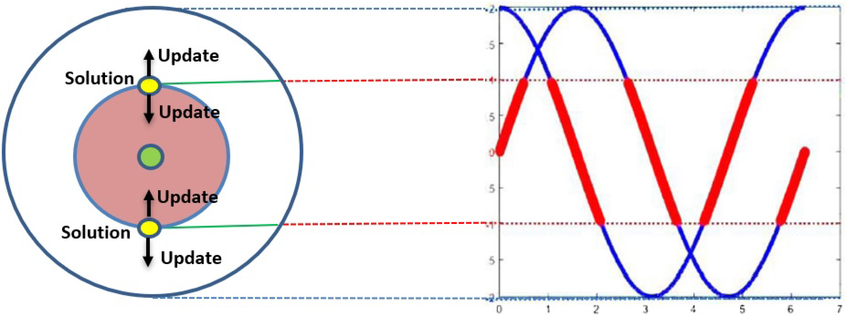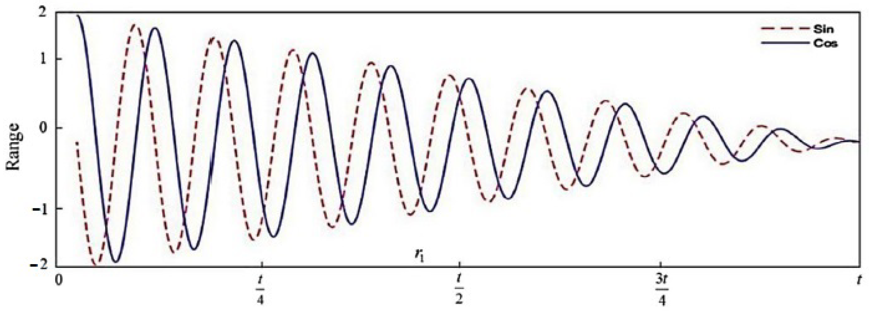Figure 8 demonstrates the switching mechanism between sine and cosine algorithms with the range in [−2, 2]. The exploration process in SCA is guaranteed in this range, since each solution may update its location outside the feasible search space.

Any metaheuristic algorithm should achieve a proper trade-off between exploration and exploitation processes. In SCA, this balance between exploration and exploitation through optimization is obtained by decreasing the range of sine and cosine, as shown in Equation (14).

$$r_1=a-k\frac{a}{K}$$

(14)

where variables k and K represent current, and maximum iterations, respectively. a is a constant.Figure 9 explores the way of decreasing the range of the sine and cosine after a set of iterations at $a=3$. Algorithm 3 presents the pseudo-code of the SCA algorithm.

Algorithm 3 Pseudo-code of SCA.

Initialize a random population of search agents (solutions) (X) Evaluate all solutions by the objective function P= the optimal solution found so far. while ($k<K$) do     Update $r_1$, $r_2$, $r_3$ and $r_4$     for each search agent in the population do         if ($r_4<0.5$) then            $X_i^{k+1}=X_i^k+r_1\times sin(r_2)\times |r_3{P}_i^k-X_i^k|$         else if ($r_4$$\ge 0.5$) then            $X_i^{k+1}=X_i^k+r_1\times cos(r_2)\times |r_3{P}_i^k-X_i^k|$     Estimate the value of objective function for each search agent.     Update P     k=k+1. returnP

3.5. Enhanced Whale Optimization Algorithm

In this subsection, we are using the concepts of the three methods mentioned above (i.e., WOA, SCA, and LCM) to propose a new hybrid algorithm that improves the overall performance of WOA. In the original WOA, the position vector of a whale (solution) is updated in the exploration stage with respect to the position vector of a randomly chosen search agent rather than the optimal search agent discovered so far. As a result, the performance of the exploration process is excellent, while the performance of the exploitation process is weak. This weakness also comes from selecting the updating mechanism (i.e., spiral-path and shrinking-circles path), which is performed randomly. To overcome this weakness, LCM is employed to ensure that $50\%$ of the iterations go for each updating mechanism.

Since SCA benefits from superior exploitation [79] and the exploration occurs once the obtained value from sine or cosine function is larger than 1 and smaller than −1, we adopted the SCA to enhance the worst half of the population in WAO after each iteration. The worst half of the population is considered as an initial population for SCA. This will improve the exploitation of WOA. Algorithm 4 shows the proposed enhanced WOA (EWOA).

Algorithm 4 Pseudo-code of EWOA.

Initialize a random population of whales Initialize all coefficients Evaluate all solutions using fitness function Determine The optimal solution so far (denoted as $X^{*}$) while (k < maximum number of iterations) do     for each solution (whale) do         Update a, A, C, l, and p coefficients.         p= LCM()         if (p < 0.5) then            if $|A|<1$ then                Update the current solution’s position by Eq.(2).            else if $|A|\ge 1$ then                Pick a random solution from the population                Update the position of $X(k)$ using Eq.(9)         else if (p≥ 0.5) then            Update the position of $X(k)$ by Eq.(7)     Estimate the fitness value for each solution (whale) in the population.     Apply SCA on worst half of the population.     Update $X^{*}$     $k=k+1$ return$X^{*}$

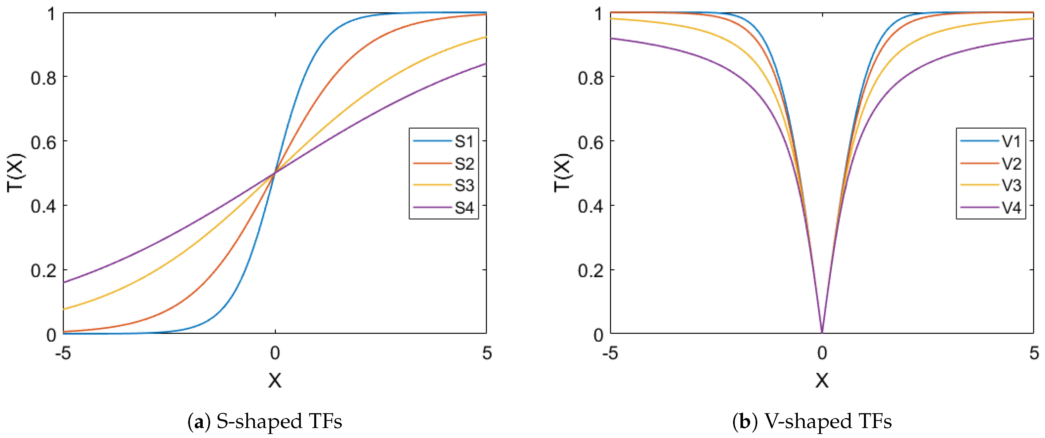
3.6. Transfer Functions to Develop Binary Variant of WOA

WOA is a continuous search algorithm by nature. Therefore, it is not applicable in its original form to deal with FS which is a binary optimization problem. Accordingly, it is imperative to convert WOA to a binary structure by utilizing a binarization scheme. Transfer Function (TF) is deemed as one of the most frequently applied binarization schemes [80,81]. For this purpose, we employed eight different TFs form two well-know groups that are S-shaped and V-shaped [81] (see Figure 10) to develop a binary variant of WOA for the FS problem. In the TF-based binarization scheme, two steps are performed. In the first step, a TF function is employed to convert the real-valued solution $R^n$ into an intermediate normalized solution $I=(I_1,I_2,\cdots ,I_n)$ within [0,1] such that each element in I represent the probability of transforming the corresponding element in $R^n$ into 0 or 1. In the second step, a binarization rule is used to convert the output of TF into binary. In the literature, the most common binarization rules are called standard method given in Equation (15) and complement method given in Equation (18). Broadly, The standard rule is used with S-shaped TFs while the complement rule is used with V-shaped TFs [82].

Considering S2 sigmoid function, the probability of updating the generated real-valued solution of WOA into binary is presented in Equation (15).

$$S(x_i^j(k))=\frac{1}{1+{exp}^{-x_i^j(k)}}$$

(15)

where $X_i^j$ is a variable that represents the jth element of the ith real-valued solution X, k represents the current iteration. The updating process for S-shape group is presented in Equation (16) for the next iteration.

$$x_i^j(k+1)=\left\{\begin{array}{cc}0\hfill & \mathrm{If}rand<S(X_i^j(k))\hfill \\ 1\hfill & \mathrm{If}rand\ge S(X_i^j(k))\hfill \end{array}\right.$$

(16)

where $X_i^j(k+1)$ represents the binary value of the corresponding $X_i^j$, and the $S(X_j^i(k))$ is the probability value that is evaluated based on Equation (15).

The updating process for V-shape for the forthcoming iteration is presented in Equation (18), which is evaluated based on the probability values that is illustrated in Equation (17) [83].

Table 1. S-shaped and V-shaped transfer functions.

S-Shaped Family		V-Shaped Family
Name	Transfer Function	Name	Transfer Function
S1	$S(x)=\frac{1}{1+e^{-2x}}$	V1	$V(x)=|\mathrm{erf}(\frac{\sqrt{\Pi }}{2}x)|=|{\frac{\sqrt{2}}{\Pi }}_0^{(\sqrt{\Pi }/2)x}{e}^{-t^2}dt|$
S2	$S(x)=\frac{1}{1+e^{-x}}$	V2	$V(x)=|tanh(x)|$
S3	$S(x)=\frac{1}{1+e^{(-x/2)}}$	V3	$V(x)=|(x)/\sqrt{1+x^2}|$
S4	$S(x)=\frac{1}{1+e^{(-x/3)}}$	V4	$V(x)=|\frac{2}{\Pi }\mathrm{arc}\tan (\frac{\Pi }{2}x)|$

explores the mathematical models for S-shape and V-shape TFs functions.

$$V(x_i^j(k))=|tanh(x_i^j(k))|$$

(17)

$$x_i^j(k+1)=\left\{\begin{array}{cc}\neg x_i^j(k)\hfill & r<V(x_i^j(k))\hfill \\ x_i^j(k)\hfill & r\ge V(x_i^j(k))\hfill \end{array}\right.$$

(18)

where ∽ is the complement. With the complement binarization rule, the new binary value ($x_i^j(k+1)$ is set considering the current binary solution, that is to say, based on the probability value $V(x_i^j(k))$, the jth element is either kept or flipped.

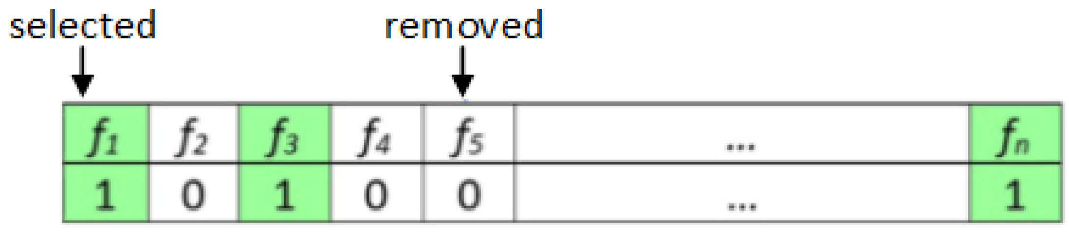
3.7. Whale Optimization Algorithm as a Feature Selection

Adapting metaheuristic algorithms to handle any optimization problem requires identifying two fundamental parts, including solution encoding and evaluation (fitness) function. Employing WOA as a binary feature selection algorithm means that the potential solution (i.e., features subset) is is expressed as a binary vector with length n (see Figure 11), where n presents the number of features in the original dataset. Each cell inside the binary vector has either 1 (i.e., selected feature) or 0 (i.e., not selected).

The main objective of the FS process is to find the smallest features subset that leads to achieving the maximum classification accuracy. Accordingly, FS can be defined as a complex multi-objective optimization problem. Aggregation is deemed one of the most common prior procedures where multiple objectives are combined into a single function. Each objective is assigned a weight to decide its significance [84]. A good ratio between selected features and classification accuracy should be achieved to have a robust FS algorithm. So, the minimization fitness function used in this work is presented in Equation (19) to assess the appropriateness of the selected subset of features.

$$\downarrow Fitness(X)=\alpha C_{ER}+\beta \frac{|S|}{|N|}$$

(19)

where $Fitness(X)$ is the fitness value of the subset X, $C_{ER}$ represents the classification error rate for the employed internal classifier using the subset X. S refers to the number selected features. N refers to the total number of features in the original dataset. $\alpha \in$ [0,1], whereas $\beta =\left(1-\alpha \right)$ are adopted from [82,85,86].

4. Student Performance Datasets

In this paper, we adopted two public datasets for student performance prediction. The first dataset (Data1) proposed by [87] in 2008. The second dataset (Data2) was obtained from Gazi University in Ankara (Turkey) [88]. The following subsections describe both datasets.

4.1. Data1

This dataset was obtained from two Portuguese secondary schools. It contains 33 features (inputs) such as demographic data, grades, social features, etc. The dataset is collected based on school mark reports, and well-structured questionnaires [87]. The dataset contains information about two subjects: Mathematics (mat) and Portuguese language (por). The main objective of this data is to predict the final grade feature, which is called G3 in the dataset. In this work, we convert the final grade into a binary where value 1 for (G3 < 10), while value 0 for (G3 ≥ 10). For more details about this dataset, interested readers can read [87]. In this work, we normalized all input features into [0,1] as a pre-processing step. We used the Portuguese language for training, whereas the Mathematics data for testing our trained models.

4.2. Data2

The second dataset contains 32 input features (i.e., 28 features represent course-specific questions and four additional features) and a single output feature (i.e., a number representing the number of times the course is repeated). All input features are normalized into [0,1], to make sure that all values are in a common scale, without having differences in the ranges of values [89]. Since we are working on a binary classification problem, we converted the output to 0 if the student repeats the course 0 or 1 time and to 1 if the student repeats the course more than 1. Interested readers about this data can explore the dataset’s official website http://archive.ics.uci.edu/ml/datasets/turkiye+student+evaluation, accessed on 8 January 2021.

4.3. Datasets Summary

Table 2. Details of student evaluation datasets.

Dataset	#Features	#Instances	Class
			Target	Binary Values	Minority Class	%Minority
Data1	32	1044	G3	0: pass, 1: fail	1: fail	0.22
Data2	32	5820	repeat	1, 0: > 1	repeat > 1	0.156

explores the details of each dataset. It is clear that both datasets are imbalanced. For example, in Data1, the minority class is 1, while the majority class is 0. The minority class for Data2 is 1 (i.e., repeat > 1), which is 0.156% of the whole dataset. As a result, it is important to handle this problem as a pre-processing step to avoid overfitting problem during the learning process. Appendix A explores the Data1 and Data2 features descriptions.

Figure 12 presents The 2D visualization for the two applied datasets based on Principle Component Analysis (PCA). It can be observed that the imbalance level of the data is high. In addition, liner separation of the data is not possible. Therefore, more sophisticated learning classifiers are needed to obtain better performance.

5. Performance Evaluation

There are several criteria to evaluate binary classification methods, including accuracy, precision, recall, F-measure, and area under ROC curve (AUC). All these criteria are affected by a cut-off value on the predicted probability of the student performance except the AUC criteria. In general, the devalue cut-off value is $0.5$, which may not be a suitable value while examining the performance of a classifier [90]. As a result, the AUC measure is not related to the cut-off value, which makes it a more suitable criterion to evaluate binary classification methods [91,92].

Moreover, ROC curves are not affected by any changes in class distributions. The AUC value is determined based on the relation between True Positive (TP) rate vs. False Positive (FP) rate. A confusion matrix is used to evaluate the final AUC value, as shown in

Table 3. The confusion matrix.

	Predicted Class
Actual Class		Class = Yes	Class = No
	Class = Yes	True Positive (TP)	False Negative (FN)
	Class = No	False Positive (FP)	True Negative (TN)

.

$$Sensitivity=T{P}_{rate}=\frac{TP}{P}$$

(20)

$$Specificity=T{N}_{rate}=\frac{TN}{N}$$

(21)

where P and N are variables present the actual positive and negative samples, respectively. Finally, AUC criteria helps researchers to generalize the obtained results [93].

6. Experimental Results and Simulations

In this section, we have performed extensive experiments to evaluate the performance of the proposed enhanced version of WOA for resolving the problem of students’ performance prediction. We examined the effect of re-sampling and feature selection on the performance of several machine learning classifiers. In addition, the performance of WOA and Enhanced WOA with S-Shaped and V-Shaped TFs is also investigated. We also compared the performance of the best variants of EWOA with other well-regarded algorithms in terms of AUC, selected features, and fitness values.

6.1. Experimental Setup

For both tested datasets, we used a K-fold cross-validation method for training and evaluating the proposed method with k = 5. Compared to the simple hold-out validation, the K-fold cross-validation has the advantage of approximating the generalization error. It allows the users to test all the data by using different folds of training and testing sets. Thus each sample has the chance of being appeared in the training and testing set [21,94].

All the optimizers were investigated using the same common settings (swarm size = 20, maximum iterations = 70, $\alpha$ = 0.99, $\beta$ = 0.01, Number of runs = 10). The internal parameters of the applied algorithms were selected according to trials and errors on small simulations and recommended settings in the literature [82]. For instance, Mirjalili and Lewis [34] recommended the a parameter to be from 2 to 0, while Rashedi et al. [83] recommended the value 10 for the parameter $G_0$ in BGSA. The parameter values for the BBA algorithm were obtained from Mirjalili et al. [95].

Table 4. The detailed parameters settings.

Configuration	Value
Fitness function
$\alpha$	0.99
$\beta$	0.01
common config.
No. runs	10
Population size	20
No. iterations	70
Dimension	#features
K for cross validation	5
specific config.
$G_0$ (for BGSA)	10
a (Convergence constant for bGWO)	from 2 to 0
$Q_{min}$ Minimum frequency (for BBA)	0
$Q_{max}$ Maximum frequency (for BBA)	2
A Loudness (for BBA)	0.5
r Pulse rate (for BBA)	0.5
a (Convergence constant for WOA)	from 2 to 0
E (for HHO)	from 2 to 0
$\omega$ (for PSO)	from 0.9 to 0.2
$c_1$ and $c_2$ (for PSO	2
GA selection	Roulette Wheel Selection
Probability of mutation in GA	0.01
Probability of crossover in GA	0.9
elite size (in GA)	2
c (for BGOA)	from 0.01 to 0.00004 [b]

shows the detailed parameters settings that are used in this paper for each algorithm.

Due to the stochastic nature of meta-heuristic algorithms, each experiment is repeated 10 times, and the results are recorded in terms of average (Avg) and standard deviation (Std). In addition, the non-parametric Wilcoxon statistical test with a 5% degree of significance is also performed to detect the significant difference between the obtained results of different algorithms. The interest in non-parametric statistical analysis has grown recently in the field of computational intelligence [96].

6.2. Preliminary Experiments

The first series of experiments were employed to assess the performance of five different classifiers (i.e., kNN, DT, LDA, LB, and NB) and determine which is the most applicable approach that fits both case studies here in this work. The preliminary experiments were divided into two categories, the first experiments are to classify the datasets without any preprocessing, while the second experiments are to examine the performance of classifiers with the resampling method using different balancing ratios.

Table 5. Evaluation results of classification methods without re-sampling and without FS.

Dataset	Classifier	TPR	TNR	AUC	Accuracy
Data1	KNN	0.9649	0.6824	0.8236	0.9026
	DT	0.9329	0.7276	0.8303	0.8877
	LDA	0.9625	0.6822	0.8223	0.9007
	LB	0.9482	0.7443	0.8463	0.9033
	NB	0.9846	0.4678	0.7262	0.8708
Data2	KNN	0.2380	0.9303	0.5842	0.8220
	DT	0.2812	0.9017	0.5914	0.8046
	LDA	0.0280	0.9930	0.5105	0.8420
	LB	0.2471	0.9493	0.5982	0.8394
	NB	0.0570	0.9824	0.5197	0.8376

explores the performance of the classifiers without resampling and without FS using four measures (i.e., TPR, TNR, AUC, and accuracy), while

Table 6. The AUC results obtained by classification algorithms with different balancing ratios (without FS).

Dataset	Classifier	Ovarsampling Ratio
		0 *	0.2	0.4	0.7	1
Data1	KNN	0.8236	0.8521	0.8600	0.8590	0.8558
	DT	0.8303	0.8384	0.8360	0.8379	0.8407
	LDA	0.8223	0.8672	0.8720	0.8818	0.8794
	LB	0.8463	0.8450	0.8479	0.8499	0.8502
	NB	0.7262	0.8629	0.8503	0.8015	0.7746
Data2	KNN	0.5842	0.6210	0.6307	0.6305	0.6332
	DT	0.5914	0.5968	0.6003	0.6031	0.6045
	LDA	0.5105	0.5378	0.5946	0.6314	0.6352
	LB	0.5982	0.6066	0.6113	0.6168	0.6187
	NB	0.5197	0.5215	0.5344	0.5716	0.5685
Rank (F-Test)		4.9	3.6	2.7	2.1	1.7

* balancing ratio of 0 indicates data without re-sampling.

explores the performance of each classifier with different balancing ratios without FS.

Inspecting AUC values in Table 5, it is evident that the LB classifier outperforms all other classifiers with excellent performance for Data 1 (i.e., AUC = 0.8463) and poor performance for Data2 (i.e., AUC = 0.5982). The reported results in Table 6 after employing a re-sampling process with different oversampling ratios show that the KNN classifier has excellent performance (i.e., AUC = 0.8600) for Data 1 with oversampling ratio equals to $0.4$. In contrast, the LDA classifier shows a good performance (i.e., AUC = 0.6352) for Data2 with oversampling ratio equals to $1.0$.

Table 7. Comparison results of classification methods without oversampling and with oversampling in terms of TPR, TNR, and AUC.

Dataset	Metric	KNN		DT		LDA		LB		NB
		without	with	without	with	without	with	without	with	without	with
Data1	TPR	0.9649	0.7990	0.9329	0.9313	0.9625	0.8347	0.9482	0.9470	0.9846	0.5548
	TNR	0.6824	0.9126	0.7276	0.7500	0.6822	0.9241	0.7443	0.7535	0.4678	0.9943
	AUC	0.8236	0.8558	0.8303	0.8407	0.8223	0.8794	0.8463	0.8502	0.7262	0.7746
Data2	TPR	0.2380	0.5486	0.2812	0.3438	0.0280	0.6395	0.2471	0.3088	0.0570	0.4640
	TNR	0.9303	0.7179	0.9017	0.8652	0.9930	0.6309	0.9493	0.9286	0.9824	0.6730
	AUC	0.5842	0.6332	0.5914	0.6045	0.5105	0.6352	0.5982	0.6187	0.5197	0.5685

compares the performance of all classifiers based on three criteria (i.e., TPR, TNR, and AUC) values with and without oversampling. It is evident that the oversampling method for both cases will improve the performance of all classifiers. The performance of LDA dominates all other classifiers with re-sampling. As a result, we will adopt the LDA as a primary classifier for evaluating the performance of the proposed EWOA.

6.3. Results with Feature Selection

To examine the performance of WOA, we performed a sensitivity analysis on WOA with S2 (WOA-S2) as a transfer function using a different number of agents (whales).

Table 8. Evaluation results of WOA-S2 with different number of search agents for the re-balanced datasets.

Dataset	Metric	No. Search Agents
		5	10	20	30	40	50
Data1	AUC	0.9023	0.9030	0.9053	0.9069	0.9060	0.9048
	Features	16.9	16.5	14.5	14.3	12.3	14.1
	Fitness	0.1020	0.1012	0.0983	0.0966	0.0969	0.0987
Data2	AUC	0.6436	0.6444	0.6454	0.6462	0.6460	0.6458
	Features	20.1	19.8	19.7	19.5	19.1	19.3
	Fitness	0.3592	0.3582	0.3572	0.3563	0.3564	0.3566
Overall Rank		6.00	5.00	3.67	1.67	1.67	3.00

explores the obtained results LDA classifier with different number of agents (i.e., 5, 10, 20, 30, 40, and 50). It is evident that the performance of LDA is not stable with a different number of agents. For example, the best performance is obtained when the number of agents equals 30 for both datasets. Choosing the correct number of agents that fit wither with the problem itself and classifier is important.

6.3.1. Performance of WOA with S-Shaped TFs

In this subsection, we examine the performance of WOA with S-shape and V-shape transfer functions.

Table 9. Evaluation results of WOA using four S-shaped TFs in terms of average and standard deviation of AUC, No. selected features, and fitness values.

Dataset	Metric	WOA-S1		WOA-S2		WOA-S3		WOA-S4
		Avg	Std	Avg	Std	Avg	Std	Avg	Std
Data1	AUC	0.90613	0.00237	0.90695	0.00187	0.90512	0.00120	0.90578	0.00156
	Features	16.00	4.88	14.30	3.20	13.90	2.77	13.30	2.67
	Fitness	0.09793	0.00324	0.09659	0.00209	0.09828	0.00152	0.09743	0.00200
Data2	AUC	0.64690	0.00125	0.64625	0.00155	0.64486	0.00098	0.64438	0.00243
	Features	24.00	2.67	19.50	2.63	19.10	2.28	18.20	2.57
	Fitness	0.35707	0.00148	0.35631	0.00115	0.35756	0.00102	0.35775	0.00260
Overall Rank (F-Test)		2.67		1.83		3.00		2.50

and

Table 10. Evaluation results of WOA using four V-shaped TFs in terms of average and standard deviation of AUC, No. selected features, and fitness values.

Dataset	Metric	WOA-V1		WOA-V2		WOA-V3		WOA-V4
		Avg	Std	Avg	Std	Avg	Std	Avg	Std
Data1	AUC	0.91305	0.00121	0.91370	0.00148	0.91403	0.00163	0.91445	0.00156
	Features	1.30	0.95	1.30	0.67	1.90	1.60	1.40	0.70
	Fitness	0.08649	0.00111	0.08584	0.00138	0.08570	0.00163	0.08513	0.00157
Data2	AUC	0.65304	0.00283	0.65524	0.00054	0.65452	0.00062	0.65526	0.00050
	Features	4.10	3.48	3.00	0.00	3.00	0.00	3.00	0.00
	Fitness	0.34477	0.00387	0.34225	0.00053	0.34296	0.00062	0.34223	0.00050
Overall Rank (F-Test)		3.58		2.25		2.67		1.50

report the obtained results. The average and standard deviation are reported in each table. It is evident that the performance of WOA-S4 outperforms all other S-shape transfer functions concerning the F-Test value. Figure 13 demonstrates the convergence diagrams for Data1 and Data 2. It is clear that the convergence of WOA-S2 is more robust and can discover more areas in the search space. The performance of WOA-V4 outperforms all other V-shape transfer functions with respect to the F-Test value. Figure 14 depicts the convergence diagrams for WOA using V-shape transfer functions. It can be seen that the performance of WOA-V4 for both datasets outperforms other V-shape transfer functions.

6.3.2. Performance of WOA with V-Shaped TFs

In order to perform further analysis on the obtained results,

Table 11. p-values of the Wilcoxon test for the AUC, number of features, and fitness results of the top variant WOA-V4 versus other variants (p≤ 0.05 are presented in bold face, NaN: means Not Applicable).

Dataset	Metric	WOA-V4 VERSUS
		WAO-S1	WOA-S2	WOA-S3	WOA-S4	WAO-V1	WOA-V2	WO-V3	WOA-V4
Data1	AUC	1.81E-04	1.81E-04	1.81E-04	1.81E-04	5.85E-02	3.06E-01	3.84E-01	1
	Features	1.28E-04	1.22E-04	1.25E-04	1.29E-04	3.87E-01	6.90E-01	5.92E-01	1
	Fitness	1.82E-04	1.82E-04	1.82E-04	1.82E-04	6.94E-02	4.05E-01	3.25E-01	1
Data2	AUC	1.83E-04	1.83E-04	1.83E-04	1.83E-04	2.45E-04	9.70E-01	3.60E-03	1
	Features	6.29E-05	6.07E-05	6.16E-05	6.29E-05	3.68E-01	NaN	NaN	1
	Fitness	1.83E-04	1.83E-04	1.83E-04	1.83E-04	2.45E-04	9.70E-01	3.60E-03	1

presents a statistical analysis using the Wilcoxon test with a significance level of $0.05$. We compared all transferred functions with WOA-V4 since WOA-V4 outperforms all S-shape and V-shapes transfer functions to simplify the comparison. It is clear that the performance of WOA-V4 is not similar to all S-shape transfer functions.

6.3.3. Comparison of Top Variants WOA-S2 and WOA-V4

Table 12. Comparison of top variants WOA-S2 and WOA-V4 in terms of AUC, selected features, and fitness rates.

Dataset	Measure	AUC		No. Selected Features		Fitness
		WOA-S2	WOA-V4	WOA-S2	WOA-V4	WOA-S2	WOA-V4
Data1	Avg	0.90695	0.91445	14.30	1.40	0.09659	0.08513
	Std	0.00187	0.00156	3.19722	0.69921	0.00209	0.00157
Wilcoxon (p-value)		1.81E-04		1.22E-04		1.82E-04
Data2	Avg	0.64625	0.65526	19.50	3.00	0.35631	0.34223
	Std	0.00155	0.00050	2.62679	0.00000	0.00115	0.00050
Wilcoxon (p-value)		1.83E-04		6.07E-05		1.83E-04

reports a compression between WOA-S2 and WOA-V4 based on Average and standard deviations for AUC, number of selected features, and fitness value. It is evident that for both datasets, WOA-V4 outperforms the WOA-S2 in all measurements. Moreover, the Wilcoxon test results show that both transfer functions have a p-value less than $0.05$. Thus, from all the previous results, the performance of V-shape version 4 is more reliable with WOA for both datasets.

6.3.4. Comparison of EWOA and WOA

Table 13. Comparison between EWOA and WOA based on best TFs.

Dataset	Measure	WOA-S2		EWOA-S2		WOA-V4		EWOA-V4
		Avg	Std	Avg	Std	Avg	Std	Avg	Std
Data1	AUC	0.90695	0.00187	0.91683	0.00133	0.91445	0.00156	0.91573	0.001046
	Features	14.30	3.20	2.2	0.918937	1.40	0.70	1.70	1.251666
	Fitness	0.09659	0.00209	0.08302	0.001421	0.08513	0.00157	0.08396	0.001289
Data2	AUC	0.64625	0.00155	0.65468	0.002318	0.65526	0.00050	0.65569	0.000556
	Features	19.50	2.63	3.9	2.84605	3.00	0.00	3.00	0.00
	Fitness	0.35631	0.00115	0.34308	0.003179	0.34223	0.00050	0.34180	0.00055
Overall Rank (F-Test)		4.00		2.33		2.08		1.58

explores the obtained results based on AUC, the number of selected features, and fitness value for EWOA and WOA using the best TFs (i.e., S2 and V4). For Data 1, the performance of EWOA-S2 outperforms other methods in terms of avg. AUC (i.e., 0.91683) and fitness value (i.e., 0.8302). While the performance of EWOA-V4 outperforms other methods for Data 2. Figure 15 depicts the convergence for all methods. We employed the F-Test value to determine the best approach. The obtained results show that EWOA-4 outperforms all other methods with F-test value equals $1.58$.

6.3.5. The Most Relevant Features Selected by EWOA-V4

To explore the most relevant features that impact students’ performance, we employed ten independent runs using EWOA-V4 for both datasets.

Table 14. The selected features by EWOA-V4 for Data1 over 10 independent runs.

Selected Features				No. Features	AUC
G2				1	0.91745
G2				1	0.916222
G2				1	0.916553
Travel-time	absences	G1	G2	4	0.914523
G2				1	0.91589
G2				1	0.91589
Travel-time	absence	G1	G2	4	0.914523
G2				1	0.915276
Fjob	G2			2	0.916649
G2				1	0.914331
			average	1.7	0.91573

shows the selected features for each run over Data1. Obviously, second-period grade (G2) appears in all runs, which means that tutors should give more attention to this feature, while traveling-time, absence, and first-period grade (G1) affect the student’s performance. Moreover, the obtained average for selected features shows that at least two features have an effect, and one of them should be a second-period grade (G2).

Table 15. The selected features by EWOA-V4 for Data2 over 10 independent runs.

Selected Features				No. Features	AUC
instr	Attendance	difficulty		3	0.655479
instr	Attendance	difficulty		3	0.656537
instr	Attendance	difficulty		3	0.655423
instr	Attendance	difficulty		3	0.655383
instr	Attendance	difficulty		3	0.655626
instr	Attendance	difficulty		3	0.656277
instr	Attendance	difficulty		3	0.655015
instr	Attendance	difficulty		3	0.656254
instr	Attendance	difficulty		3	0.654896
instr	Attendance	difficulty		3	0.656017
			average	3.0	0.65569

explores the selected features for Data2. From the reported results, three features (i.e., instr, Attendance, and difficulty) are the most relevant features that tutors should pay attention to them to predict students’ performance. Finally,

Table 16. The most relevant features selected by EWOA-V4 based on the total number of selections over 10 independent runs.

Dataset	Sequence #	Feature	Number of Selections	Ratio
Data1	31	G2	10	100%
	13	Travel-time	2	20%
	30	absences	2	20%
	31	G1	2	20%
	10	Fjob	1	10%
Data2	1	instr	10	100%
	3	attendance	10	100%
	4	difficulty	10	100%

summarizes the selected features for each dataset based on the number of selections and ratios. We believe that each educational organization should examine their data carefully to find the most relevant features that affect their students’ performance.

6.4. Comparison of EWOA with Other Well-Known Algorithms

After performing extensive experiments to prove the efficiency of EWOA over the conventional WOA, we validate its performance by comparing it with a set of well-regarded algorithms, namely Binary Harris Hawks Optimization (BHHO) [97], Binary Gravitational Search Algorithm (BGSA) [98], Binary Grasshopper Optimisation Algorithm (BGOA) [99], Binary Particle Swarm Optimization (BPSO) [100], Binary Grey Wolf Optimizer (BGWO) [101], Binary Bat Algorithm (BBA) [102], Binary Ant Lion Optimizer (BALO) [103], and Genetic Algorithm (GA) [104]. We adopted these competitors because they are categorized into different groups of meta-heuristic techniques. For instance, GA is evolutionary-based, GSA is physics-based, while the others are swarm-based. Hence each algorithm has its exploratory and exploitative potentials. Moreover, these algorithms have been successfully applied as wrapper FS approaches in different domains. To make a fair comparison, ADASYN was used with all competing approaches.

Table 17. Comparison of the proposed approaches with other well-regarded algorithms in terms of AUC, selected features, and fitness values.

Dataset	Metric		EWOA-S2	EWOA-V4	BHHO	BGSA	BGOA	BPSO	BGWO	BBA	GA	BALO
Data1	AUC	AVG	0.91683	0.91573	0.89627	0.89053	0.89762	0.90332	0.90508	0.86580	0.89977	0.89124
		STD	0.00133	0.00105	0.00629	0.00760	0.00939	0.00624	0.00483	0.06794	0.00734	0.00486
	Features	AVG	2.2	1.7	13.1	14.5	13.2	10.5	5.5	14.4	10.8	22.5
		STD	0.91894	1.25167	2.51440	2.22361	2.52982	2.27303	1.84089	2.63312	2.82056	5.25463
	Fitness	AVG	0.08302	0.08396	0.09518	0.09882	0.09354	0.09195	0.08562	0.09850	0.09693	0.10179
		STD	0.00142	0.00129	0.00222	0.00291	0.00261	0.00178	0.00217	0.00196	0.00285	0.00137
Data2	AUC	AVG	0.65468	0.65569	0.63839	0.63735	0.63671	0.64021	0.63917	0.61790	0.63980	0.63752
		STD	0.00232	0.00056	0.00355	0.00409	0.00502	0.00315	0.00246	0.02016	0.00240	0.00444
	Features	AVG	3.9	3	19.2	16.8	18.4	15.7	11.8	17	15	26.1
		STD	2.84605	0.00000	3.58391	1.93218	2.59058	2.21359	2.74064	1.33333	1.63299	3.21282
	Fitness	AVG	0.34308	0.34180	0.35585	0.35707	0.35651	0.35460	0.35096	0.35946	0.35853	0.35892
		STD	0.00318	0.00055	0.00124	0.00218	0.00137	0.00128	0.00124	0.00342	0.00111	0.00092
Overall rank (F-Test)			1.67	1.33	6.5	8	6.83	4	3.33	8.83	5.5	9

presents a deep comparison between all approaches in terms of average AUC, number of features, and fitness values with STD values and the F-test ranking. The reported results clarify that the proposed EWOA-S2 and EWOA-V4 exceed the other algorithms in achieving higher ACU rates with fewer features on the utilized datasets. Accordingly, the proposed EWOA efficiently keeps the most informative features that offer better classification performance in dealing with student performance prediction. Based on the overall ranking, the EWOA-V4 outperforms all other methods with the rank of $1.33$. It is ranked as the best performing method in terms of the considered metrics. Moreover, EWOA-S2 comes in second place with a mean rank of $1.67$. In contrast, the performance of BBA is the worst one (rank of $8.83$).

Figure 16 illustrates the convergence curves of the developed EWOA-V4 versus other methods. Obviously, EWOA-V4 achieves a better acceleration trend in dealing with both datasets. The diverse exploratory and exploitative behaviors in the developed EWOA-V4 improve its ability to explore the targeted space and converge faster toward better solutions.

6.5. Comparison with State-of-the-Art Approaches

To further validate the results of the proposed method, it is compared with nine state-of-the-art methods in [89] using the G-mean measure (G-mean is the reported measure in this study). Considering the results in

Table 18. Validation of our proposed method with the proposed methods by [89] in terms of G-mean measure.

Approach	Data1	Data2
our approach	0.9146	0.6548
Method1-Opt1	0.7495	0.7256
Method1-Opt2	0.7486	0.7276
Method2-Opt1	0.7488	0.7267
Method2-Opt2	0.7478	0.7259
Original-RVFL	0.7113	0.6887
Imp-RVFL-KDE	0.7242	0.7068
Imp-RVFL-MCC	0.7257	0.7072
Imb-RVFL-Opt1	0.7198	0.7158
Imb-RVFL-Opt2	0.7217	0.7123

, the superiority and competitiveness of the proposed method is evident again. Furthermore, we compared the proposed method with the best results achieved in the study of Thaher and Jayousi [14] and Alraddadi et al. [15] in terms of AUC measure. As in

Table 19. Comparison of the proposed approach with similar studies in terms of AUC.

Dataset	MLP-Adam [14]	BTLBO-LDA [15]	Our Approach
Data1	0.8201	-	0.9157
Data2	0.6052	0.6323	0.6557

, it can be seen that our proposed approach achieved the best AUC rates compared to results presented in previous studies on the same datasets.

Taken together, the experiments and comparative results demonstrated the merits of the proposed WOA methods. The superiority of the proposed methods are due the several reasons. Firstly, the exploitation of WOA was improved using the SCA algorithm. It has been demonstrated several times in the literature that SCA’s exploitation is its main strength, so the accuracy of results obtained in this work are due to the use of SCA in conjunction with WOA. Despite high exploitative, the algorithm perform well on high-dimensional data sets too, which are very challenging due to the large number of locally optimal solutions. This is due use of chaotic maps and different transfer functions what allow the proposed method to show diverse exploratory behaviours.

7. Conclusions and Future Works

In this work, an enhanced approach as a wrapper feature selection that combines the Whale Optimization Algorithm (WOA) with Sine Cosine Algorithm (SCA) is introduced. The main idea is to enhance the performance of the WOA exploitation process by improving the worst half in the population based on the SCA algorithm at every iteration. In addition, to enhance the population diversity and increase the exploratory behaviour of WOA, chaotic sequence number generated by logistic chaotic map is employed to balance between two updating mechanisms (i.e., spiral-path and shrinking-circles path) inside the WOA.

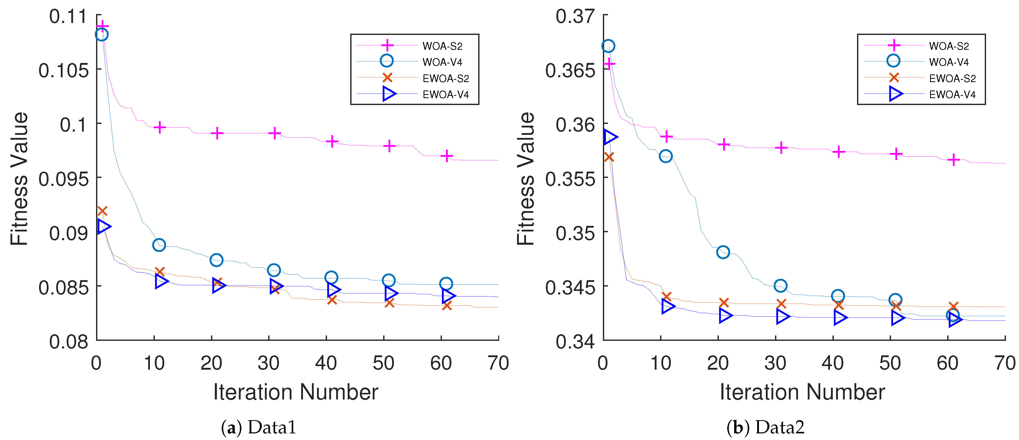
The performance of the proposed algorithm was examined on educational data come from two different schools. Five different classifiers have been examined (i.e., k-NN, DT, LDA, NB, and LB). The performance of LDA outperforms other classifiers with respect to the AUC value. The performance of EWOA with V4 TF (EWOA-V4) shows an outstanding performance compared to other algorithms in the literature.

The limitation of this work is the availability of students’ performance datasets, where few datasets are available for research. Another limitation of this work is that the proposed enhanced WOA has only been tested in the SPP domain. In addition, the parameters of the algorithms were set based on small simulations and common settings in the literature. In future works, we will examine the performance of the proposed approach in multi-objective optimization problems and more complex data such as medical and biological datasets. We will also conduct extensive experiments to determine the most appropriate values of common and internal parameters for the enhanced WOA as well as other utilized algorithms.

References

1. Marwaha, A.; Singla, A. A study of factors to predict at-risk students based on machine learning techniques. In Intelligent Communication, Control and Devices; Choudhury, S., Mishra, R., Mishra, R.G., Kumar, A., Eds.; Springer: Singapore, 2020; pp. 133–141. [Google Scholar]
2. Trstenjak, B.; Đonko, D. Determining the impact of demographic features in predicting student success in croatia. In Proceedings of the 2014 37th International Convention on Information and Communication Technology, Electronics and Microelectronics (MIPRO), Opatija, Croatia, 26–30 May 2014; pp. 1222–1227. [Google Scholar] [CrossRef]
3. Mallikarjun Rao, B.; Ramana Murthy, B.V. Prediction of student’s educational performance using machine learning techniques. In Data Engineering and Communication Technology; Raju, K.S., Senkerik, R., Lanka, S.P., Rajagopal, V., Eds.; Springer: Singapore, 2020; pp. 429–440. [Google Scholar]
4. Crespo-Turrado, C.; Casteleiro-Roca, J.L.; Sánchez-Lasheras, F.; López-Vázquez, J.A.; De Cos Juez, F.J.; Pérez Castelo, F.J.; Calvo-Rolle, J.L.; Corchado, E. Comparative study of imputation algorithms applied to the prediction of student performance. Log. J. IGPL 2019, 28, 58–70. [Google Scholar] [CrossRef]
5. Tomasevic, N.; Gvozdenovic, N.; Vranes, S. An overview and comparison of supervised data mining techniques for student exam performance prediction. Comput. Educ. 2020, 143, 103676. [Google Scholar] [CrossRef]
6. Kaur, P.; Singh, M.; Josan, G.S. Classification and prediction based data mining algorithms to predict slow learners in education sector. Procedia Comput. Sci. 2015, 57, 500–508. [Google Scholar] [CrossRef] [Green Version]
7. Bogarín, A.; Romero, C.; Cerezo, R.; Sánchez-Santillán, M. Clustering for improving educational process mining. In Proceedings of the Fourth International Conference on Learning Analytics And Knowledge, Indianapolis, IN, USA, 24–28 March 2014; ACM: New York, NY, USA, 2014; pp. 11–15. [Google Scholar] [CrossRef]
8. Abdullah, Z.; Herawan, T.; Ahmad, N.; Deris, M.M. Mining significant association rules from educational data using critical relative support approach. Procedia-Soc. Behav. Sci. 2011, 28, 97–101. [Google Scholar] [CrossRef] [Green Version]
9. Romero, C.; Ventura, S.; Zafra, A.; de Bra, P. Applying Web usage mining for personalizing hyperlinks in Web-based adaptive educational systems. Comput. Educ. 2009, 53, 828–840. [Google Scholar] [CrossRef]
10. Polyzou, A.; Karypis, G. Feature extraction for next-term prediction of poor student performance. IEEE Trans. Learn. Technol. 2019, 12, 237–248. [Google Scholar] [CrossRef]
11. Adekitan, A.I.; Salau, O. The impact of engineering students’ performance in the first three years on their graduation result using educational data mining. Heliyon 2019, 5, e01250. [Google Scholar] [CrossRef] [PubMed] [Green Version]
12. Fernandes, E.; Holanda, M.; Victorino, M.; Borges, V.; Carvalho, R.; Erven, G.V. Educational data mining: Predictive analysis of academic performance of public school students in the capital of Brazil. J. Bus. Res. 2019, 94, 335–343. [Google Scholar] [CrossRef]
13. Jääskelä, P.; Heilala, V.; Kärkkäinen, T.; Häkkinen, P. Student agency analytics: Learning analytics as a tool for analysing student agency in higher education. Behav. Inf. Technol. 2020, 40, 790–808. [Google Scholar] [CrossRef]
14. Thaher, T.; Jayousi, R. Prediction of student’s academic performance using feedforward neural network augmented with stochastic trainers. In Proceedings of the 2020 IEEE 14th International Conference on Application of Information and Communication Technologies (AICT), Tashkent, Uzbekistan, 7–9 October 2020; pp. 1–7. [Google Scholar] [CrossRef]
15. Alraddadi, S.; Alseady, S.; Almotiri, S. Prediction of students academic performance utilizing hybrid teaching-learning based feature selection and machine learning models. In Proceedings of the 2021 International Conference of Women in Data Science at Taif University (WiDSTaif ), Taif, Saudi Arabia, 30–31 March 2021; pp. 1–6. [Google Scholar] [CrossRef]
16. Han, J.; Kamber, M.; Pei, J. Data Mining: Concepts and Techniques; Elsevier, Morgan Kaufmann Publishers: Amsterdam, The Netherlands, 2012. [Google Scholar]
17. Mafarja, M.; Mirjalili, S. Hybrid whale optimization algorithm with simulated annealing for feature selection. Neurocomputing 2017, 260, 302–312. [Google Scholar] [CrossRef]
18. Liu, H.; Motoda, H. Feature Selection for Knowledge Discovery and Data Mining; Springer: Berlin/Heidelberg, Germany, 2012; Volume 454. [Google Scholar]
19. Chantar, H.K.; Corne, D.W. Feature subset selection for Arabic document categorization using BPSO-KNN. In Proceedings of the 2011 Third World Congress on Nature and Biologically Inspired Computing, Salamanca, Spain, 19–21 October 2011; pp. 546–551. [Google Scholar]
20. Chantar, H.; Thaher, T.; Turabieh, H.; Mafarja, M.; Sheta, A. BHHO-TVS: A binary harris hawks optimizer with time-varying scheme for solving data classification problems. Appl. Sci. 2021, 11, 6516. [Google Scholar] [CrossRef]
21. Tumar, I.; Hassouneh, Y.; Turabieh, H.; Thaher, T. Enhanced binary moth flame optimization as a feature selection algorithm to predict software fault prediction. IEEE Access 2020, 8, 8041–8055. [Google Scholar] [CrossRef]
22. Wang, A.; An, N.; Chen, G.; Li, L.; Alterovitz, G. Accelerating wrapper-based feature selection with K-nearest-neighbor. Knowl.-Based Syst. 2015, 83, 81–91. [Google Scholar] [CrossRef]
23. Saeys, Y.; Iñaki, I.; Pedro, L.n. A review of feature selection techniques in bioinformatics. Bioinformatics 2007, 23, 2507–2517. [Google Scholar] [CrossRef] [Green Version]
24. Dash, M.; Liu, H. Feature selection for classification. Intell. Data Anal. 1997, 1, 131–156. [Google Scholar] [CrossRef]
25. Siedlecki, W.; Sklansky, J. On automatic feature selection. Int. J. Pattern Recognit. Artif. Intell. 1988, 2, 197–220. [Google Scholar] [CrossRef]
26. Langley, P. Selection of relevant features in machine learning. In Proceedings of the AAAI Fall symposium on Relevance; Association for the Advancement of Artificial Intelligence: Menlo Park, CA, USA, 1994; Volume 184, pp. 245–271. [Google Scholar]
27. Lai, C.; Reinders, M.J.; Wessels, L. Random subspace method for multivariate feature selection. Pattern Recognit. Lett. 2006, 27, 1067–1076. [Google Scholar] [CrossRef]
28. Talbi, E. Metaheuristics From Design to Implementation; John Wiley & Sons: Hoboken, NJ, USA, 2009. [Google Scholar]
29. Guyon, I.; Elisseeff, A. An introduction to variable and feature selection. J. Mach. Learn. Res. 2003, 3, 1157–1182. [Google Scholar]
30. Zorarpacı, E.; Özel, S.A. A hybrid approach of differential evolution and artificial bee colony for feature selection. Expert Syst. Appl. 2016, 62, 91–103. [Google Scholar] [CrossRef]
31. Kennedy, J.; Eberhart, R.C. A discrete binary version of the particle swarm algorithm. In Proceedings of the 1997 IEEE International Conference on Systems, Man, and Cybernetics. Computational Cybernetics and Simulation, Orlando, FL, USA, 12–15 October 1997; Volume 5, pp. 4104–4108. [Google Scholar]
32. Dorigo, M.; Birattari, M.; Stutzle, T. Ant colony optimization. IEEE Comput. Intell. Mag. 2006, 1, 28–39. [Google Scholar] [CrossRef]
33. Deriche, M. Feature selection using ant colony optimization. In Proceedings of the 2009 6th International Multi-Conference on Systems, Signals and Devices, Djerba, Tunisia, 23–26 March 2009; pp. 1–4. [Google Scholar] [CrossRef]
34. Mirjalili, S.; Lewis, A. The whale optimization algorithm. Adv. Eng. Softw. 2016, 95, 51–67. [Google Scholar] [CrossRef]
35. Hassouneh, Y.; Turabieh, H.; Thaher, T.; Tumar, I.; Chantar, H.; Too, J. Boosted whale optimization algorithm with natural selection operators for software fault prediction. IEEE Access 2021, 9, 14239–14258. [Google Scholar] [CrossRef]
36. Gui-Ying, N.; Cao, D.Q. Improved whale optimization algorithm for solving constrained optimization problems. Discret. Dyn. Nat. Soc. 2021, 2021, 1–13. [Google Scholar] [CrossRef]
37. Ding, T.; Chang, L.; Li, C.; Feng, C.; Zhang, N. A mixed-strategy-based whale optimization algorithm for parameter identification of hydraulic turbine governing systems with a delayed water hammer effect. Energies 2018, 11, 2367. [Google Scholar] [CrossRef] [Green Version]
38. Abdel-Basset, M.; Abdle-Fatah, L.; Kumar, A. An improved Lévy based whale optimization algorithm for bandwidth-efficient virtual machine placement in cloud computing environment. Clust. Comput. 2019, 22, 8319–8334. [Google Scholar] [CrossRef]
39. Tubishat, M.; Abushariah, M.A.; Idris, N.; Aljarah, I. Improved whale optimization algorithm for feature selection in arabic sentiment analysis. Appl. Intell. 2019, 49, 1688–1707. [Google Scholar] [CrossRef]
40. Baker, R.S.; Yacef, K. The state of educational data mining in 2009: A review and future visions. J. Educ. Data Min. 2009, 1, 3–17. [Google Scholar]
41. Aldowah, H.; Al-Samarraie, H.; Fauzy, W.M. Educational data mining and learning analytics for 21st century higher education: A review and synthesis. Telemat. Inform. 2019, 37, 13–49. [Google Scholar] [CrossRef]
42. Campagni, R.; Merlini, D.; Sprugnoli, R.; Verri, M.C. Data mining models for student careers. Expert Syst. Appl. 2015, 42, 5508–5521. [Google Scholar] [CrossRef]
43. Francis, B.K.; Babu, S.S. Predicting academic performance of students using a hybrid data mining approach. J. Med. Syst. 2019, 43, 162. [Google Scholar] [CrossRef]
44. Turabieh, H.; Azwari, S.; Rokaya, M.; Alosaimi, W.; Alharbi, A.; Alhakami, W.; Alnefaie, M. Enhanced harris hawks optimization as a feature selection for the prediction of student performance. Computing 2021, 103, 1–22. [Google Scholar] [CrossRef]
45. Al-Radaideh, Q.; Al-Shawakfa, E.; Al-Najjar, M. International Arab Conference on Information Technology (ACIT’2006); Yarmouk University: Irbid, Jordan, 2006. [Google Scholar]
46. Ahmad, F.; Ismail, N.H.; Aziz, A.A. The prediction of students’ academic performance using classification data mining techniques. Appl. Math. Sci. 2015, 9, 6415–6426. [Google Scholar] [CrossRef]
47. Hamsa, H.; Indiradevi, S.; Kizhakkethottam, J. Student academic performance prediction model using decision tree and fuzzy genetic algorithm. Procedia Technol. 2016, 25, 326–332. [Google Scholar] [CrossRef] [Green Version]
48. Asogbon, M.; Samuel, O.; Omisore, O.; Ojokoh, B. A multi-class support vector machine approach for students academic performance prediction. Int. J. Multidiscip. Curr. Res. 2016, 4, 210–215. [Google Scholar]
49. Guleria, P.; Sood, M. Classifying educational data using support vector machines: A supervised data mining technique. Indian J. Sci. Technol. 2016, 9. [Google Scholar] [CrossRef]
50. Burman, I.; Som, S. Predicting students academic performance using support vector machine. In Proceedings of the 2019 Amity International Conference on Artificial Intelligence (AICAI), Dubai, United Arab Emirates, 4–6 February 2019; pp. 756–759. [Google Scholar] [CrossRef]
51. Kesumawati, A.; Utari, D.T. Predicting patterns of student graduation rates using Naïve bayes classifier and support vector machine. AIP Conf. Proc. 2018, 2021, 060005. [Google Scholar]
52. Shaziya, H. Prediction of students performance in semester exams using a naïve bayes classifier. Int. J. Innov. Res. Sci. Eng. Technol. 2018, 4, 9823–9829. [Google Scholar] [CrossRef]
53. Makhtar, M.; Nawang, H.; Shamsuddin, S.N. Analysis on students performance using naÏve Bayes classifier. J. Theor. Appl. Inf. Technol. 2017, 95, 3993–4000. [Google Scholar]
54. Yang, F.; Li, F.W. Study on student performance estimation, student progress analysis, and student potential prediction based on data mining. Comput. Educ. 2018, 123, 97–108. [Google Scholar] [CrossRef] [Green Version]
55. Rana, S.; Garg, R. Student’s performance evaluation of an institute using various classification algorithms. In Information and Communication Technology for Sustainable Development; Mishra, D.K., Nayak, M.K., Joshi, A., Eds.; Springer: Singapore, 2018; pp. 229–238. [Google Scholar]
56. Amrieh, E.; Hamtini, T.; Aljarah, I. Mining educational data to predict student’s academic performance using ensemble methods. Int. J. Database Theory Appl. 2016, 9, 119–136. [Google Scholar] [CrossRef]
57. Jain, A.K.; Dubes, R.C. Algorithms for Clustering Data; Prentice-Hall, Inc.: Hoboken, NJ, USA, 1988. [Google Scholar]
58. Dutt, A.; Aghabozrgi, S.; Ismail, M.A.B.; Mahroeian, H. Clustering algorithms applied in educational data mining. Int. J. Inf. Electron. Eng. 2015, 5, 112. [Google Scholar] [CrossRef] [Green Version]
59. Harwati; Alfiani, A.P.; Wulandari, F.A. Mapping student’s performance based on data mining approach (A Case Study). Agric. Agric. Sci. Procedia 2015, 3, 173–177. [Google Scholar] [CrossRef] [Green Version]
60. Park, Y.; Yu, J.H.; Jo, I.H. Clustering blended learning courses by online behavior data: A case study in a Korean higher education institute. Internet High. Educ. 2016, 29, 1–11. [Google Scholar] [CrossRef]
61. Valsamidis, S.; Kontogiannis, S.; Kazanidis, I.; Theodosiou, T.; Karakos, A. A clustering methodology of web log data for learning management systems. J. Educ. Technol. Soc. 2012, 15, 154–167. [Google Scholar]
62. Baker, R.S.; Inventado, P.S. Educational data mining and learning analytics. In Learning Analytics: From Research to Practice; Larusson, J.A., White, B., Eds.; Springer: New York, NY, USA, 2014; pp. 61–75. [Google Scholar] [CrossRef] [Green Version]
63. Simpson, K.; Beukelman, D.; Sharpe, T. An elementary student with severe expressive communication impairment in a general education classroom: Sequential analysis of interactions. Augment. Altern. Commun. 2000, 16, 107–121. [Google Scholar] [CrossRef]
64. Nakamura, S.; Nozaki, K.; Morimoto, Y.; Miyadera, Y. Sequential pattern mining method for analysis of programming learning history based on the learning process. In Proceedings of the 2014 International Conference on Education Technologies and Computers (ICETC), Lodz, Poland, 22–24 September 2014; pp. 55–60. [Google Scholar] [CrossRef]
65. Tarus, J.K.; Niu, Z.; Yousif, A. A hybrid knowledge-based recommender system for e-learning based on ontology and sequential pattern mining. Future Gener. Comput. Syst. 2017, 72, 37–48. [Google Scholar] [CrossRef]
66. Rojas, J.A.; Espitia, H.E.; Bejarano, L.A. Design and optimization of a fuzzy logic system for academic performance prediction. Symmetry 2021, 13, 133. [Google Scholar] [CrossRef]
67. Lee, T.S.; Wang, C.H.; Yu, C.M. Fuzzy evaluation model for enhancing E-Learning systems. Mathematics 2019, 7, 918. [Google Scholar] [CrossRef] [Green Version]
68. Hameed, I.A. Enhanced fuzzy system for student’s academic evaluation using linguistic hedges. In Proceedings of the 2017 IEEE International Conference on Fuzzy Systems (FUZZ-IEEE), Naples, Italy, 9–12 July 2017; pp. 1–6. [Google Scholar]
69. Thaher, T.; Arman, N. Efficient multi-swarm binary harris hawks optimization as a feature selection approach for software fault prediction. In Proceedings of the 2020 11th International Conference on Information and Communication Systems (ICICS), Irbid, Jordan, 7–9 April 2020; pp. 249–254. [Google Scholar] [CrossRef]
70. He, H.; Garcia, E. Learning from imbalanced data. Knowl. Data Eng. IEEE Trans. 2009, 21, 1263–1284. [Google Scholar] [CrossRef]
71. Haibo, H.; Yang, B.; Garcia, E.A.; Shutao, L. ADASYN: Adaptive synthetic sampling approach for imbalanced learning. In Proceedings of the 2008 IEEE International Joint Conference on Neural Networks (IEEE World Congress on Computational Intelligence), Hong Kong, China, 1–8 June 2008; pp. 1322–1328. [Google Scholar] [CrossRef] [Green Version]
72. Watkins, W.A.; Schevill, W.E. Aerial observation of feeding behavior in four baleen whales: Eubalaena glacialis, Balaenoptera borealis, Megaptera novaeangliae, and Balaenoptera physalus. J. Mammal. 1979, 60, 155–163. [Google Scholar] [CrossRef]
73. Gao, S.; Yu, Y.; Wang, Y.; Wang, J.; Cheng, J.; Zhou, M. Chaotic local search-based differential evolution algorithms for optimization. IEEE Trans. Syst. Man Cybern. Syst. 2019. [Google Scholar] [CrossRef]
74. Chuang, L.Y.; Yang, C.H.; Li, J.C. Chaotic maps based on binary particle swarm optimization for feature selection. Appl. Soft Comput. 2011, 11, 239–248. [Google Scholar] [CrossRef]
75. Alatas, B. Chaotic bee colony algorithms for global numerical optimization. Expert Syst. Appl. 2010, 37, 5682–5687. [Google Scholar] [CrossRef]
76. Wang, G.G.; Guo, L.; Gandomi, A.H.; Hao, G.S.; Wang, H. Chaotic krill herd algorithm. Inf. Sci. 2014, 274, 17–34. [Google Scholar] [CrossRef]
77. Liu, B.; Wang, L.; Jin, Y.H.; Tang, F.; Huang, D.X. Improved particle swarm optimization combined with chaos. Chaos Solitons Fractals 2005, 25, 1261–1271. [Google Scholar] [CrossRef]
78. Gandomi, A.H.; Yang, X.S. Chaotic bat algorithm. J. Comput. Sci. 2014, 5, 224–232. [Google Scholar] [CrossRef]
79. Mirjalili, S. SCA: A Sine Cosine Algorithm for solving optimization problems. Knowl.-Based Syst. 2016, 96, 120–133. [Google Scholar] [CrossRef]
80. Crawford, B.; Soto, R.; Astorga, G.; García, J.; Castro, C.; Paredes, F. Putting continuous metaheuristics to work in binary search spaces. Complexity 2017, 2017. [Google Scholar] [CrossRef] [Green Version]
81. Mirjalili, S.; Lewis, A. S-shaped versus V-shaped transfer functions for binary Particle Swarm Optimization. Swarm Evol. Comput. 2013, 9, 1–14. [Google Scholar] [CrossRef]
82. Thaher, T.; Mafarja, M.; Turabieh, H.; Castillo, P.A.; Faris, H.; Aljarah, I. Teaching learning-based optimization with evolutionary binarization schemes for tackling feature selection problems. IEEE Access 2021, 9, 41082–41103. [Google Scholar] [CrossRef]
83. Rashedi, E.; Nezamabadi-pour, H.; Saryazdi, S. BGSA: Binary gravitational search algorithm. Nat. Comput. 2010, 9, 727–745. [Google Scholar] [CrossRef]
84. Mirjalili, S.; Dong, J. Multi-Objective Optimization Using Artificial Intelligence Techniques; Springer: Cham, Switzerland, 2020. [Google Scholar] [CrossRef]
85. Emary, E.; Zawbaa, H.M. Impact of chaos functions on modern swarm optimizers. PLoS ONE 2016, 11, e0158738. [Google Scholar] [CrossRef] [Green Version]
86. Faris, H.; Mafarja, M.M.; Heidari, A.A.; Aljarah, I.; Ala’M, A.Z.; Mirjalili, S.; Fujita, H. An efficient binary salp swarm algorithm with crossover scheme for feature selection problems. Knowl.-Based Syst. 2018, 154, 43–67. [Google Scholar] [CrossRef]
87. Cortez, P.; Silva, A. Using data mining to predict secondary school student performance. In Proceedings of the 5th FUture BUsiness TEChnology Conference (FUBUTEC 2008), Porto, Portugal, 9–11 April 2008; pp. 5–12. [Google Scholar]
88. Dua, D.; Graff, C. UCI Machine Learning Repository. 2019. Available online: http://archive.ics.uci.edu/ml (accessed on 8 January 2021).
89. Li, M.; Huang, C.; Wang, D.; Hu, Q.; Zhu, J.; Tang, Y. Improved randomized learning algorithms for imbalanced and noisy educational data classification. Computing 2019, 101, 571–585. [Google Scholar] [CrossRef]
90. Zhang, F.; Mockus, A.; Keivanloo, I.; Zou, Y. Towards building a universal defect prediction model with rank transformed predictors. Empir. Softw. Eng. 2016, 21, 2107–2145. [Google Scholar] [CrossRef]
91. Fawcett, T. ROC Graphs: Notes and practical considerations for researchers. Mach. Learn. 2004, 31, 1–38. [Google Scholar]
92. Ghotra, B.; McIntosh, S.; Hassan, A.E. Revisiting the impact of classification techniques on the performance of defect prediction models. In Proceedings of the 37th International Conference on Software Engineering—Volume 1, Florence, Italy, 16–24 May 2015; IEEE Press: Piscataway, NJ, USA, 2015; pp. 789–800. [Google Scholar]
93. Koru, A.G.; Emam, K.E.; Zhang, D.; Liu, H.; Mathew, D. Theory of relative defect proneness. Empir. Softw. Eng. 2008, 13, 473. [Google Scholar] [CrossRef]
94. Hastie, T.; Tibshirani, R.; Friedman, J. The Elements of Statistical Learning: Data Mining, Inference, and Prediction, 2nd ed.; Springer: New York, NY, USA, 2009. [Google Scholar]
95. Mirjalili, S.; Mirjalili, S.M.; Yang, X.S. Binary bat algorithm. Neural Comput. Appl. 2014, 25, 663–681. [Google Scholar] [CrossRef]
96. Derrac, J.; García, S.; Molina, D.; Herrera, F. A practical tutorial on the use of nonparametric statistical tests as a methodology for comparing evolutionary and swarm intelligence algorithms. Swarm Evol. Comput. 2011, 1, 3–18. [Google Scholar] [CrossRef]
97. Thaher, T.; Heidari, A.A.; Mafarja, M.; Dong, J.S.; Mirjalili, S. Binary harris hawks optimizer for high-dimensional, low sample size feature selection. In Evolutionary Machine Learning Techniques: Algorithms and Applications; Mirjalili, S., Faris, H., Aljarah, I., Eds.; Springer: Singapore, 2020; pp. 251–272. [Google Scholar] [CrossRef]
98. Rashedi, E.; Nezamabadi-pour, H. Feature subset selection using improved binary gravitational search algorithm. J. Intell. Fuzzy Syst. Appl. Eng. Technol. 2014, 26, 1211–1221. [Google Scholar] [CrossRef]
99. Mafarja, M.; Aljarah, I.; Faris, H.; Hammouri, A.I.; Al-Zoubi, A.M.; Mirjalili, S. Binary grasshopper optimisation algorithm approaches for feature selection problems. Expert Syst. Appl. 2019, 117, 267–286. [Google Scholar] [CrossRef]
100. Mafarja, M.; Jarrar, R.; Ahmed, S.; Abusnaina, A. Feature selection using binary particle swarm optimization with time varying inertia weight strategies. In Proceedings of the 2nd International Conference on Future Networks and Distributed Systems, Amman Jordan, 26–27 June 2018. [Google Scholar] [CrossRef]
101. Emary, E.; Zawbaa, H.M.; Hassanien, A.E. Binary grey wolf optimization approaches for feature selection. Neurocomputing 2016, 172, 371–381. [Google Scholar] [CrossRef]
102. Nakamura, R.Y.M.; Pereira, L.A.M.; Rodrigues, D.; Costa, K.A.P.; Papa, J.P.; Yang, X.S. 9—Binary bat algorithm for feature selection. In Swarm Intelligence and Bio-Inspired Computation; Yang, X.S., Cui, Z., Xiao, R., Gandomi, A.H., Karamanoglu, M., Eds.; Elsevier: Oxford, UK, 2013; pp. 225–237. [Google Scholar]
103. Emary, E.; Zawbaa, H.; Hassanien, A.E. Binary ant lion approaches for feature selection. Neurocomputing 2016, 213, 54–65. [Google Scholar] [CrossRef]
104. Babatunde, O.; Armstrong, L.; Leng, J.; Diepeveen, D. A genetic algorithm-based feature selection. Int. J. Electron. Commun. Comput. Eng. 2014, 5, 889–905. [Google Scholar]
Figure 1. EMD lifecycle.
Applsci 11 10237 g001
Figure 2. Proposed approach.
Applsci 11 10237 g002
Figure 3. Bubble-net feeding strategy for whale.
Applsci 11 10237 g003
Figure 4. Potential 2D and 3D locations of whales in the neighbourhood of the prey.
Applsci 11 10237 g004
Figure 5. Shrinking encircling mechanism.
Applsci 11 10237 g005
Figure 6. Spiral updating position (red circle denotes the position of prey while yellow circle is the position of a whale).
Applsci 11 10237 g006
Figure 7. Updating whale position either towards or moving away from a randomly picked humpback whale.
Applsci 11 10237 g007
Figure 8. Solution update process toward or moving away from the best solution.
Applsci 11 10237 g008
Figure 9. Decreasing pattern for the sine and cosine.
Applsci 11 10237 g009
Figure 10. Transfer functions families (a) S-shaped and (b) V-shaped.
Applsci 11 10237 g010
Figure 11. A pattern of binary solution for a dataset of n features.
Applsci 11 10237 g011
Figure 12. Visualization of distribution of the target class based on the first two principal components of the features in the dataset.
Applsci 11 10237 g012
Figure 13. Convergence curves of WOA with different S-shaped TFs.
Applsci 11 10237 g013
Figure 14. Convergence curves of WOA with different V-shaped TFs.
Applsci 11 10237 g014
Figure 15. The convergence for the EWOA and WOA using S2 and V4 TFS.
Applsci 11 10237 g015
Figure 16. Convergence curves for all compared algorithms.
Applsci 11 10237 g016