
Prescribed Performance Non-Singular Fast Terminal Sliding Mode Control Based on Extended State Observer for a Deep-Sea Electric Oil-Filled Joint Actuator


Abstract
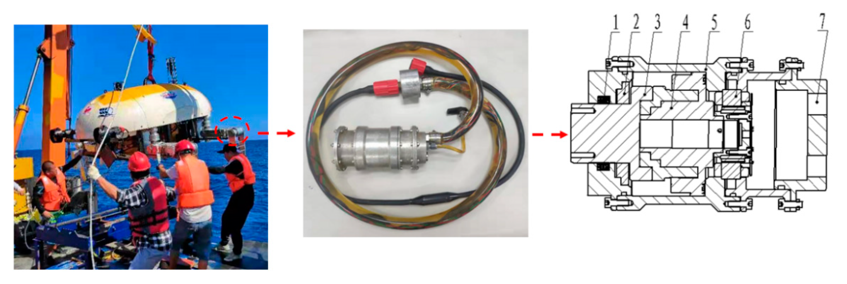
:1. Introduction
2. Dynamic Modeling and Problem Formulation
2.1. Dynamic Modeling
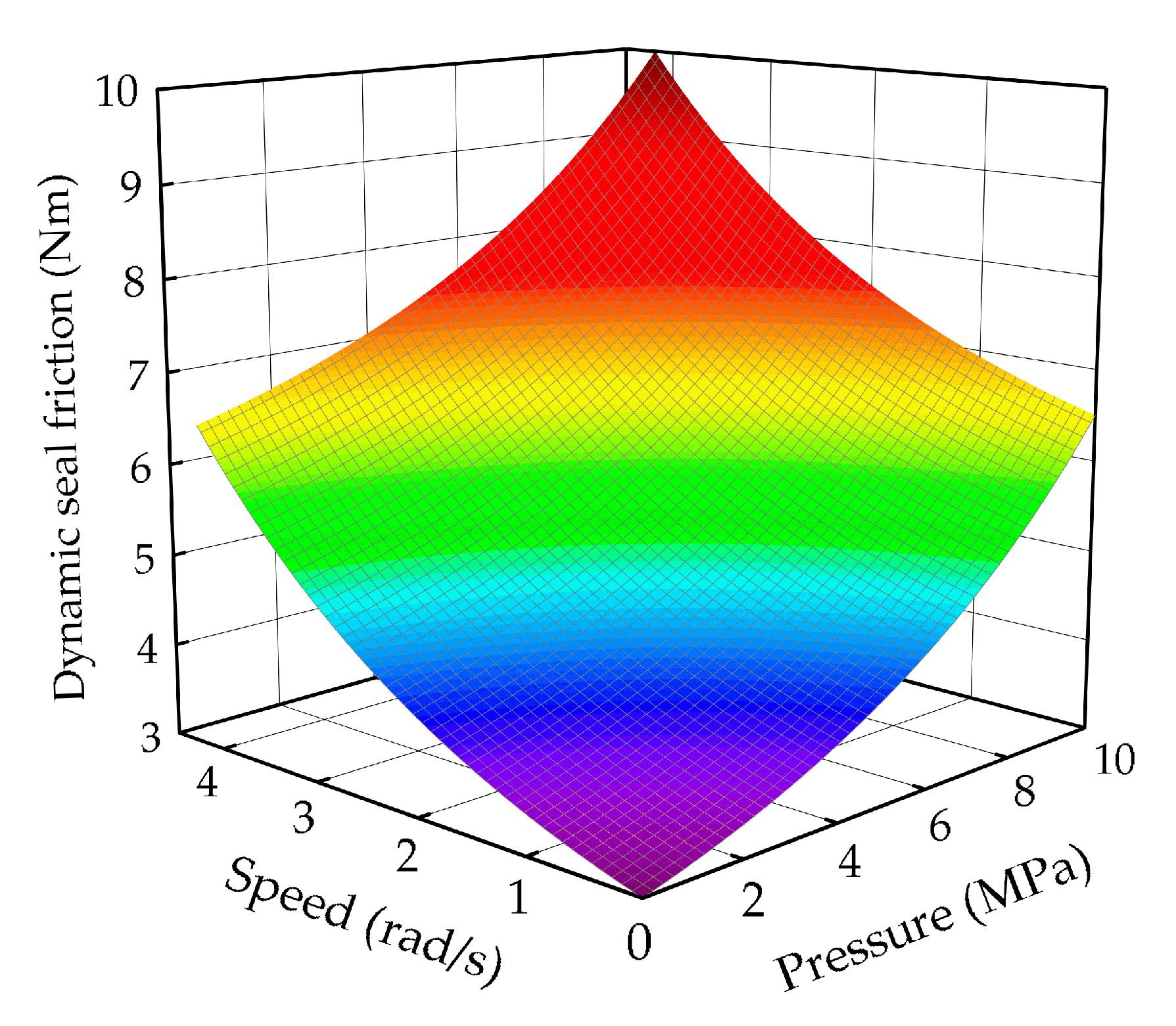
2.2. Oil Stirring Viscos Loss Modeling
2.3. Prescribed Performance Function
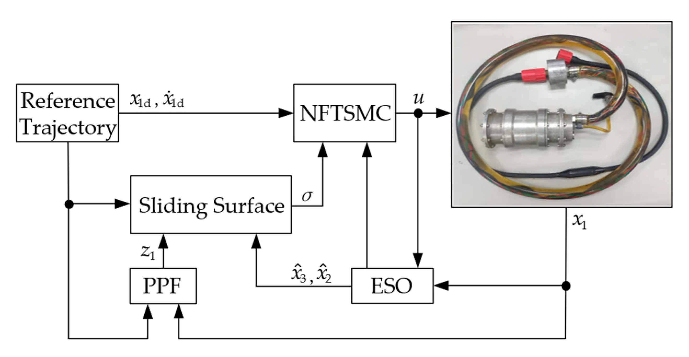
3. Extended State Observer Design
4. PP-NFTSMC-ESO Controller Design
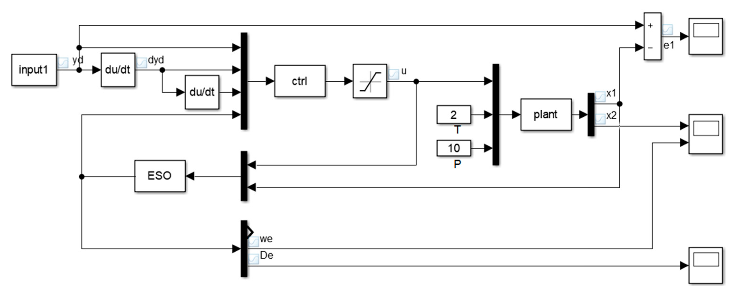
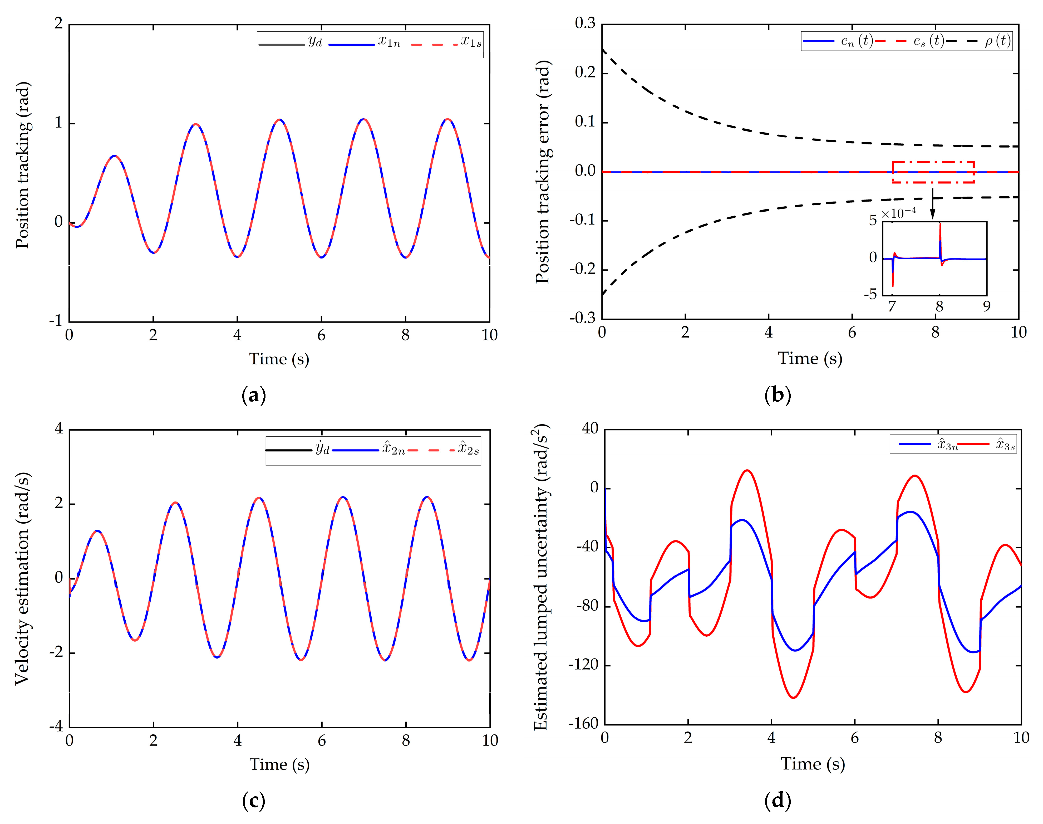
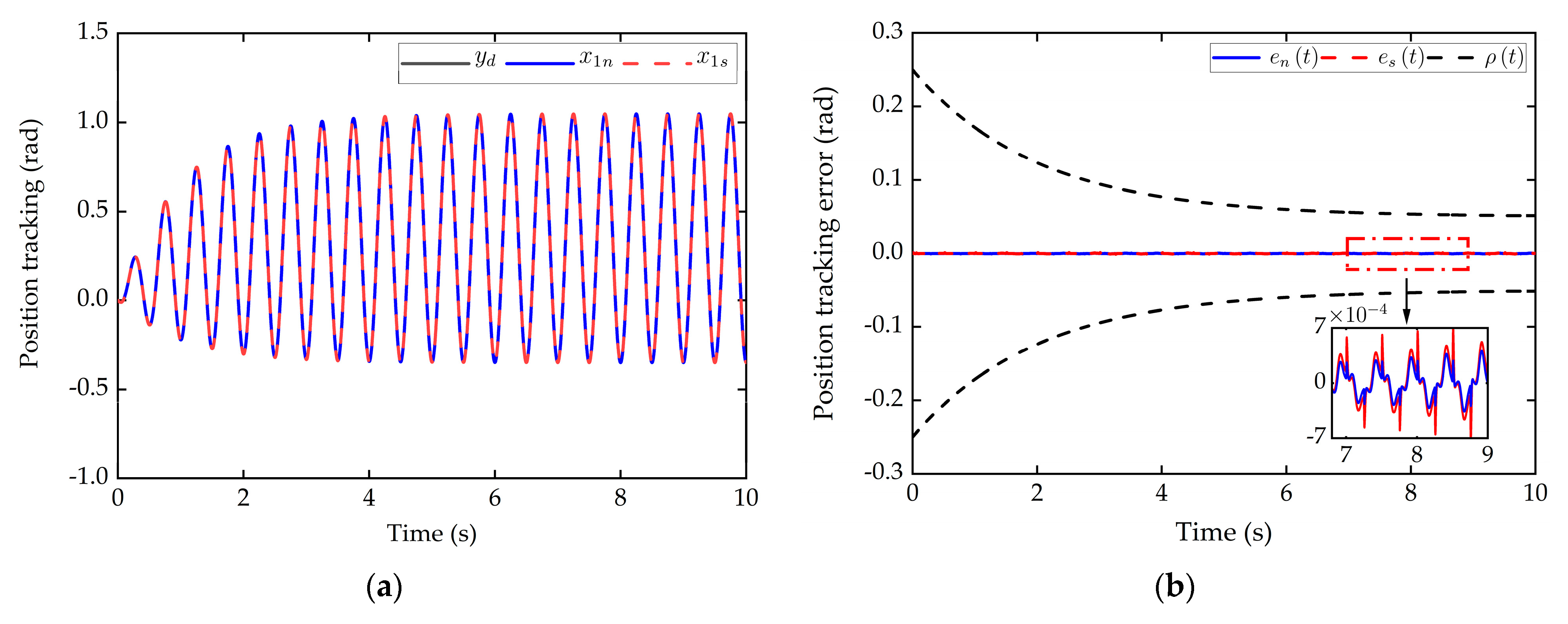
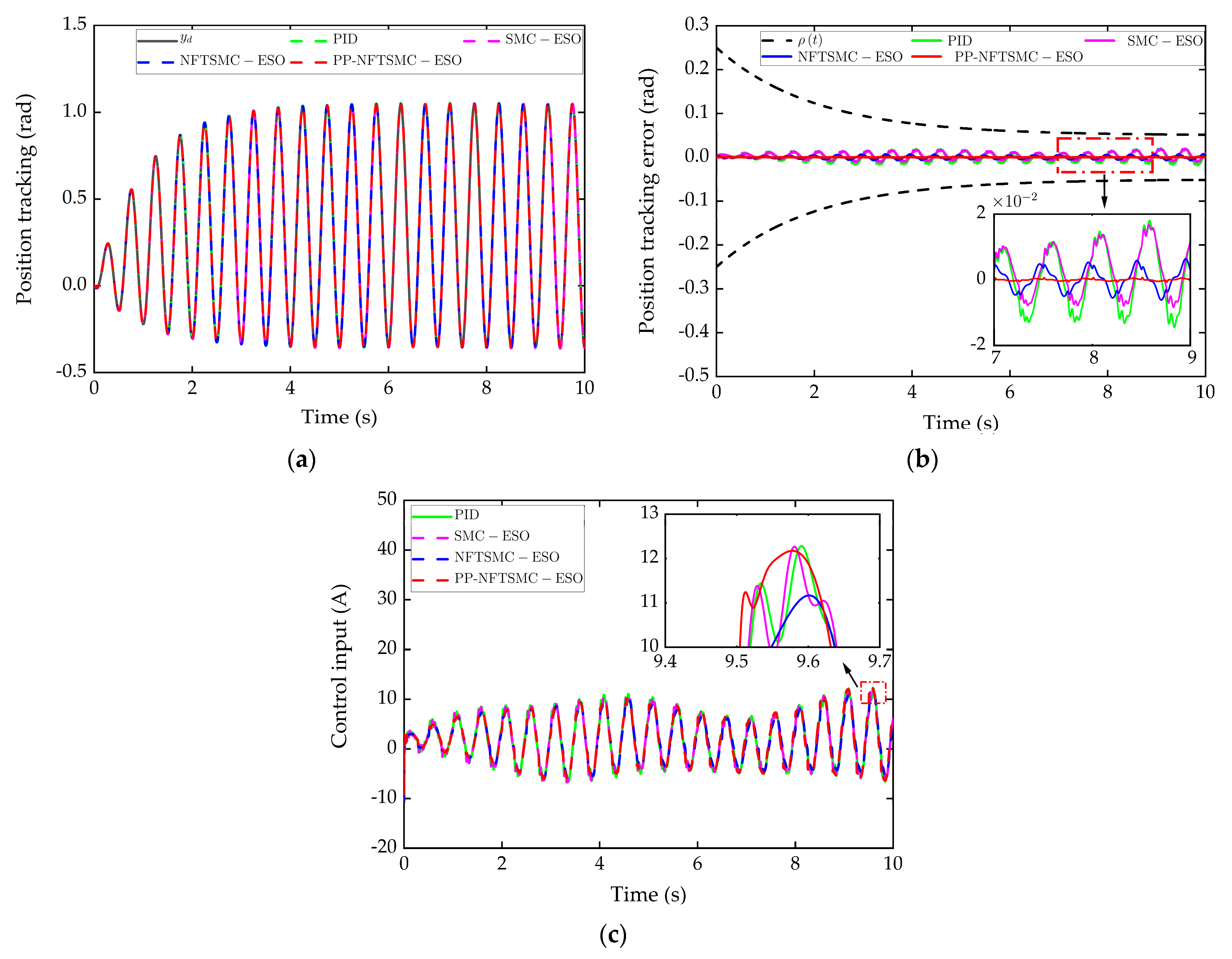
5. Numeric Simulation
5.1. Simulation Setup
5.2. Controllers for Comparison
5.3. Simulation Study
6. Conclusions
Author Contributions
Funding
Institutional Review Board Statement
Informed Consent Statement
Data Availability Statement
Acknowledgments
Conflicts of Interest
Appendix A
Appendix B
References
- Shim, H.; Yoo, Y.S.; Kang, H.; Jun, B. Development of arm and leg for seabed walking robot CRABSTER200. Ocean Eng. 2016, 116, 55–67. [Google Scholar] [CrossRef]
- Liu, Y.; Deng, Y.; Fang, M.; Li, D.; Wu, D. Research on the torque characteristics of a seawater hydraulic axial piston motor in deep-sea environment. Ocean Eng. 2017, 146, 411–423. [Google Scholar] [CrossRef]
- Sivčev, S.; Coleman, J.; Omerdić, E.; Dooly, G.; Toala, D. Underwater manipulators: A review. Ocean Eng. 2018, 163, 431–450. [Google Scholar] [CrossRef]
- Ribas, D.; Ridao, P.; Turetta, A.; Melchiorri, C.; Palli, G.; Fernández, J.; Sanz, P. I-AUV mechatronics integration for the TRIDENT FP7 project. IEEE/ASME Trans. Mechatron. 2015, 20, 2583–2592. [Google Scholar] [CrossRef]
- Fernandez, J.; Prats, M.; Sanz, P.; Garcia, J.; Marin, R.; Robinson, M.; Ribas, D.; Ridao, P. Grasping for the seabed: Developing a new underwater robot arm for shallow-water intervention. IEEE Robot. Autom. Mag. 2013, 20, 121–130. [Google Scholar] [CrossRef]
- Li, G.; Chen, X.; Zhou, F.; Liang, Y.; Xiao, Y.; Cao, X.; Yang, W. Self-powered soft robot in the Mariana Trench. Nature 2021, 591, 66–71. [Google Scholar] [CrossRef]
- Bai, Y.; Zhang, Q.; Zhang, A. Modeling and Optimization of Compensating Oil Viscous Power for a Deep-Sea Electric Manipulator. IEEE Access 2021, 18, 13524–13531. [Google Scholar] [CrossRef]
- Cai, M.; Wu, S.; Yang, C. Effect of Low Temperature and High Pressure on Deep-Sea Oil-Filled Brushless DC Motors. Mar. Technol. Soc. J. 2016, 50, 83–93. [Google Scholar] [CrossRef]
- Zou, J.; Qi, W.; Xu, Y.; Xu, F.; Li, Y.; Li, J. Design of Deep Sea Oil-Filled Brushless DC Motors Considering the High Pressure Effect. IEEE Trans. Magn. 2012, 48, 4220–4223. [Google Scholar] [CrossRef]
- Stevenson, P.; Hunter, C. Development of an Efficient Propulsion Motor and Driver for Use in the Deep Ocean. In Proceedings of the International Conference on Electronic Engineering in Oceanography IET, Cambridge, UK, 19–21 July 1994; pp. 51–55. [Google Scholar]
- Accetta, A.; Cirrincione, M.; Pucci, M.; Vitale, G. Neural Sensorless Control of Linear Induction Motors by a Full-Order Luenberger Observer Considering the End Effects. IEEE Trans. Ind. Appl. 2014, 50, 1891–1904. [Google Scholar] [CrossRef]
- Li, Z.; Zhou, S.; Xiao, Y.; Wang, L. Sensorless Vector Control of Permanent Magnet Synchronous Linear Motor Based on Self-Adaptive Super-Twisting Sliding Mode Controller. IEEE Access 2019, 7, 44998–45011. [Google Scholar] [CrossRef]
- Liu, H.; Nie, J.; Sun, J.; Tian, X. Adaptive Super-Twisting Sliding Mode Control for Mobile Robots Based on High-Gain Observers. J. Control. Sci. Eng. 2020, 2020, 4048507. [Google Scholar] [CrossRef]
- Xu, Z.; Zhang, T.; Bao, Y.; Zhang, H.; Gerada, C. A Nonlinear Extended State Observer for Rotor Position and Speed Estimation for Sensorless IPMSM Drives. IEEE Trans. Power Electron. 2020, 35, 733–743. [Google Scholar] [CrossRef]
- Liu, J.; Gao, Y.; Su, X.; Wack, M.; Wu, L. Disturbance-observer-based control for air management of PEM fuel cell systems via sliding mode technique. IEEE Trans. Control Syst. Technol. 2019, 27, 1129–1138. [Google Scholar] [CrossRef]
- Mohanty, A.; Yao, B. Indirect Adaptive Robust Control of Hydraulic Manipulators with Accurate Parameter Estimates. IEEE Trans. Control Syst. Technol. 2011, 19, 567–575. [Google Scholar] [CrossRef]
- Yao, J.; Jiao, Z.; Ma, D. Adaptive Robust Control of DC Motors with Extended State Observer. IEEE Trans. Ind. Electron. 2014, 61, 3630–3637. [Google Scholar] [CrossRef]
- Wang, Z.; Hu, C.; Zhu, Y.; He, S.; Yang, K.; Zhang, M. Neural Network Learning Adaptive Robust Control of an Industrial Linear Motor-Driven Stage with Disturbance Rejection Ability. IEEE Trans. Ind. Inform. 2017, 13, 2172–2183. [Google Scholar] [CrossRef]
- Kamaldin, N.; Chen, S.; Teo, C.; Lin, W.; Tan, K. A Novel Adaptive Jerk Control with Application to Large Workspace Tracking on a Flexure-Linked Dual-Drive Gantry. IEEE Trans. Ind. Electron. 2019, 66, 5353–5363. [Google Scholar] [CrossRef]
- Sun, X.; Yu, H.; Yu, J.; Liu, X. Design and implementation of a novel adaptive backstepping control scheme for a PMSM with unknown load torque. IET Electr. Power Appl. 2019, 13, 445–455. [Google Scholar] [CrossRef]
- Wang, Y.; Yan, F.; Chen, J.; Ju, F.; Chen, B. A New Adaptive Time-Delay Control Scheme for Cable-Driven Manipulators. IEEE Trans. Ind. Inform. 2019, 15, 3469–3481. [Google Scholar] [CrossRef]
- Shao, K.; Zheng, J.; Huang, K.; Wang, H.; Man, Z.; Fu, M. Finite-Time Control of a Linear Motor Positioner Using Adaptive Recursive Terminal Sliding Mode. IEEE Trans. Ind. Electron. 2020, 67, 6659–6668. [Google Scholar] [CrossRef]
- Yao, J.; Jiao, Z.; Ma, D.; Yan, L. High-Accuracy Tracking Control of Hydraulic Rotary Actuators with Modeling Uncertainties. IEEE/ASME Trans. Mechatron. 2014, 19, 633–641. [Google Scholar] [CrossRef]
- Yao, B.; Hu, C.; Lu, L.; Wang, Q. Adaptive Robust Precision Motion Control of a High-Speed Industrial Gantry with Cogging Force Compensations. IEEE Trans. Control Syst. Technol. 2011, 19, 1149–1159. [Google Scholar] [CrossRef]
- Wang, J.; Wang, F.; Wang, G.; Li, S.; Yu, L. Generalized Proportional Integral Observer Based Robust Finite Control Set Predictive Current Control for Induction Motor Systems with Time-Varying Disturbances. IEEE Trans. Ind. Inform. 2018, 14, 4159–4168. [Google Scholar] [CrossRef]
- Shi, D.; Xue, J.; Zhao, L.; Wang, J.; Huang, Y. Event-Triggered Active Disturbance Rejection Control of DC Torque Motors. IEEE/ASME Trans. Mechatron. 2017, 22, 2277–2287. [Google Scholar] [CrossRef]
- Yin, Z.; Bai, C.; Du, N.; Du, C.; Liu, J. Research on Internal Model Control of Induction Motors Based on Luenberger Disturbance Observe. IEEE Trans. Power Electron. 2021, 36, 8155–8170. [Google Scholar] [CrossRef]
- Liao, L.; Li, B.; Wang, Y.; Xi, Y.; Zhang, D.; Gao, L. Adaptive Fuzzy Robust Control of a Bionic Mechanical Leg with a High Gain Observer. IEEE Access 2021, 9, 134037–134051. [Google Scholar] [CrossRef]
- Son, Y.; Kim, I.; Choi, D.; Shim, H. Robust Cascade Control of Electric Motor Drives Using Dual Reduced-Order PI Observer. IEEE Trans. Ind. Electron. 2015, 62, 3672–3682. [Google Scholar] [CrossRef]
- Nguyen, V.; Vo, A.; Kang, H. A Non-Singular Fast Terminal Sliding Mode Control Based on Third-Order Sliding Mode Observer for a Class of Second-Order Uncertain Nonlinear Systems and its Application to Robot Manipulators. IEEE Access 2020, 8, 78109–78120. [Google Scholar] [CrossRef]
- Xue, W.; Bai, W.; Yang, S.; Song, K.; Huang, Y.; Xie, H. ADRC With Adaptive Extended State Observer and its Application to Air–Fuel Ratio Control in Gasoline Engines. IEEE Trans. Ind. Electron. 2015, 62, 5847–5857. [Google Scholar] [CrossRef]
- Li, M.; Zhao, J.; Hu, Y.; Wang, Z. Active disturbance rejection position servo control of PMSLM based on reduced-order extended state observer. Chin. J. Electr. Eng. 2020, 6, 30–41. [Google Scholar] [CrossRef]
- Komurcugil, H.; Ozdemir, S.; Sefa, I.; Altin, N.; Kukrer, O. Sliding-Mode Control for Single-Phase Grid-Connected LCL-Filtered VSI with Double-Band Hysteresis Scheme. IEEE Trans. Ind. Electron. 2016, 63, 864–873. [Google Scholar] [CrossRef]
- Eker, I. Sliding mode control with PID sliding surface and experimental application to an electromechanical plant. ISA Trans. 2006, 45, 109–118. [Google Scholar] [CrossRef]
- Vo, A.; Kang, H. An adaptive terminal sliding mode control for robot manipulators with non-singular terminal sliding surface variables. IEEE Access 2019, 7, 8701–8712. [Google Scholar] [CrossRef]
- Wang, H.; Man, Z.; Kong, H.; Zhao, Y.; Yu, M.; Cao, Z.; Zheng, J.; Do, M. Design and implementation of adaptive terminal sliding-mode control on a Steer-by-Wire equipped road vehicle. IEEE Trans. Ind. Electron. 2016, 63, 5774–5785. [Google Scholar] [CrossRef]
- Truong, T.; Vo, A.; Kang, H. A Backstepping Global Fast Terminal Sliding Mode Control for Trajectory Tracking Control of Industrial Robotic Manipulators. IEEE Access 2021, 9, 31921–31931. [Google Scholar] [CrossRef]
- Vo, A.; Kang, H. An Adaptive Neural Non-Singular Fast-Terminal Sliding-Mode Control for Industrial Robotic Manipulators. Appl. Sci. 2018, 8, 2562. [Google Scholar] [CrossRef] [Green Version]
- Zhao, X.; Fu, D. Adaptive Neural Network Nonsingular Fast Terminal Sliding Mode Control for Permanent Magnet Linear Synchronous Motor. IEEE Access 2019, 7, 180361–180372. [Google Scholar] [CrossRef]
- Chen, G.; Jin, B.; Chen, Y. Nonsingular fast terminal sliding mode posture control for six-legged walking robots with redundant actuation. Mechatronics 2018, 50, 1–15. [Google Scholar] [CrossRef]
- Zheng, J.; Wang, H.; Man, Z.; Jin, J.; Fu, M. Robust Motion Control of a Linear Motor Positioner Using Fast Nonsingular Terminal Sliding Mode. IEEE/ASME Trans. Mechatron. 2015, 20, 1743–1752. [Google Scholar] [CrossRef]
- Zhang, L.; Wei, C.; Wu, R.; Cui, N. Fixed-time extended state observer based non-singular fast terminal sliding mode control for a VTVL reusable launch vehicle. Aerosp. Sci. Technol. 2018, 82–83, 70–79. [Google Scholar] [CrossRef]
- Zhang, J.; Wang, H.; Cao, Z.; Zheng, J.; Yu, M.; Yazdani, A.; Shahnia, F. Fast nonsingular terminal sliding mode control for permanent-magnet linear motor via ELM. Neural Comput. Appl. 2020, 32, 14447–14457. [Google Scholar] [CrossRef]
- Liu, Y.; Laghrouche, S.; N’Diaye, A.; Cirrincione, M. Hermite neural network-based second-order sliding-mode control of synchronous reluctance motor drive systems. J. Frankl. Inst. 2021, 358, 400–427. [Google Scholar] [CrossRef]
- Xu, Z.; Liu, Q.; Yao, J. Adaptive prescribed performance control for hydraulic system with disturbance compensation. Int. J. Adapt. Control. Signal Process. 2021, 35, 1544–1561. [Google Scholar] [CrossRef]
- Na, J.; Chen, Q.; Ren, X.; Guo, Y. Adaptive prescribed performance motion control of servo mechanisms with friction compensation. IEEE Trans. Ind. Electron. 2014, 61, 486–494. [Google Scholar] [CrossRef]
- Wang, P.; Wang, J.; Ming, S.; Chang, L. Prescribed performance back-stepping robustness control of a flexible hypersonic vehicle. Electr. Mach. Control 2017, 21, 94–102. [Google Scholar]
- Zheng, Q.; Gaol, L.; Gao, Z. On stability analysis of active disturbance rejection control for nonlinear time-varying plants with unknown dynamics. In Proceedings of the 46th IEEE Conference on Decision and Control, New Orleans, LA, USA, 12–14 December 2007; pp. 3501–3506. [Google Scholar]
- Gao, Z. Scaling and bandwidth-parameterization based controller tuning. In Proceedings of the 2003 American Control Conference, Denver, CO, USA, 4–6 June 2003; pp. 4989–4996. [Google Scholar]

| Parameter | ||||
|---|---|---|---|---|
| value | 3.34 × 10⁻⁵ | 0.105 | 1.95 × 10⁻⁵ | 100 |
| Parameter | 1 | ||
|---|---|---|---|
| value | 2 °C | 140.3 | |
| 25 °C | 41.6 | ||
| Parameter | d | h | L | |||
|---|---|---|---|---|---|---|
| value | 37.5 mm | 63 mm | 37.5 mm | 0.3 mm | 38 mm | 15.5 mm |
| Controller/Observer | Parameter |
|---|---|
| PI | |
| SMC-ESO | |
| NFTSMC-ESO | |
| PP-NFTSMC-ESO | |
| ESO |
| Normal Laboratory Working Condition | Deep-Sea Working Condition | |
|---|---|---|
| slow motion | 2.55 × 10⁻⁴ rad | 4.89 × 10⁻⁴ rad |
| fast motion | 4.36 × 10⁻⁴ rad | 6.96 × 10⁻⁴ rad |
| Controller | Maximum Steady State Tracking Error (rad) |
|---|---|
| PI | 1.84 × 10⁻² |
| SMC-ESO | 1.71 × 10⁻² |
| NFTSMC-ESO | 6.64 × 10⁻³ |
| PP-NFTSMC-ESO | 6.96 × 10⁻⁴ |
Publisher’s Note: MDPI stays neutral with regard to jurisdictional claims in published maps and institutional affiliations. |
© 2021 by the authors. Licensee MDPI, Basel, Switzerland. This article is an open access article distributed under the terms and conditions of the Creative Commons Attribution (CC BY) license (https://creativecommons.org/licenses/by/4.0/).
Share and Cite
Liao, L.; Li, B.; Wang, Y.; Tang, T.; Zhang, D.; Yang, G. Prescribed Performance Non-Singular Fast Terminal Sliding Mode Control Based on Extended State Observer for a Deep-Sea Electric Oil-Filled Joint Actuator. Appl. Sci. 2021, 11, 10130. https://doi.org/10.3390/app112110130
Liao L, Li B, Wang Y, Tang T, Zhang D, Yang G. Prescribed Performance Non-Singular Fast Terminal Sliding Mode Control Based on Extended State Observer for a Deep-Sea Electric Oil-Filled Joint Actuator. Applied Sciences. 2021; 11(21):10130. https://doi.org/10.3390/app112110130
Chicago/Turabian StyleLiao, Lihui, Baoren Li, Yuanyuan Wang, Tengfei Tang, Dijia Zhang, and Gang Yang. 2021. "Prescribed Performance Non-Singular Fast Terminal Sliding Mode Control Based on Extended State Observer for a Deep-Sea Electric Oil-Filled Joint Actuator" Applied Sciences 11, no. 21: 10130. https://doi.org/10.3390/app112110130
APA StyleLiao, L., Li, B., Wang, Y., Tang, T., Zhang, D., & Yang, G. (2021). Prescribed Performance Non-Singular Fast Terminal Sliding Mode Control Based on Extended State Observer for a Deep-Sea Electric Oil-Filled Joint Actuator. Applied Sciences, 11(21), 10130. https://doi.org/10.3390/app112110130