Abstract
Six degree-of-freedom (6-DOF) robotic manipulators have been increasingly adopted in various applications in industries due to various advantages, such as large operation space, more degrees of freedom, low cost, easy placement, and convenient programming. However, the robotic manipulator has the problem of insufficient stiffness due to the series structures, which will cause motion errors of the manipulator end. In this paper, taking a 6-DOF robotic manipulator as an example, forward and inverse kinematics models are established, and a new modeling method for the joint angle and space stiffness of the end of the manipulator is proposed, which can establish the composite stiffness model of joint link stiffness and joint stiffness. An error compensation model is subsequently established. The experimental results indicate that the proposed error compensation method can effectively reduce the end motion error of the robotic manipulator, and hence, the working performance and accuracy of the manipulator can be improved. The proposed research is helpful for extending the application of robotic manipulators in precision machining and measurement.
1. Introduction
Since the advent of robots in the 1940s, robot technology has constantly improved. After nearly a century of development, this technology has become an indispensable part of industries and production, especially in the field of precision machining and testing [1,2]. However, due to their series structure configuration, robotic manipulators have some problems, such as jitter and a relatively large end error caused by insufficient stiffness. To improve the stiffness and working performance of robots, many researchers have carried out relevant research during the past few decades. Tan [3] obtained an estimate of each joint stiffness of an industrial robot by analyzing the joint rigidity of the mechanical transmission system structure and parameters of conversion. Based on the analysis of joint stiffness and arm stiffness, Liu [4] employed the error model to establish the stiffness model of industrial robots. In 2011, Dumas et al. [5] from France established the static stiffness model of industrial robots and proposed the relevant joint stiffness identification method with the condition that the complementary stiffness matrix term and infinite stiffness of the robot connecting rod were disregarded. In 2013, Lahmann et al. [6] from Russia used the data measured by sensors inside the robot to identify the joint stiffness of the robot. Ailon et al. [7] pointed out that the stiffness at the end of a robot would change with its posture. In 2015, Kilimchik et al. [8] in France converted the flexibility of the arm to the flexibility of joints, established the robot stiffness model, and then identified the stiffness parameters by considering the flexibility of the manipulator and joints. In 2018, Wang et al. [9] proposed the concept of an offset stiffness matrix, explored the impact of the offset stiffness matrix on milling, and verified its correctness. Lin et al. [10] proposed a vibration control method using a tunable mass damper with variable stiffness, which could avoid the maladjustment effect and suppress the vibration.
For the space stiffness of a tandem manipulator composed of traditional joints, much research has been conducted. Ye et al. [11] utilized the bionic method of the human spine to calculate the stiffness matrix of a 6-DOF manipulator to improve its accuracy. Geng et al. [12] proposed a continuous manipulator driven by a variable stiffness wire that could be passively adapted to collision and ensure operation accuracy. Liao et al. [13] proposed a region-based tool path generation method to improve the stiffness in the robot milling of freeform surfaces. Based on the matrix structure analysis method, Ali et al. [14] expounded the calculation method of the Cartesian stiffness matrix of the manipulator and introduced a new performance index of the manipulator. Jhan et al. [15] proposed an adaptive impedance force control method for manipulators based on a fuzzy neural network and estimated the stiffness coefficient of the contact environment. Han et al. [16] combined the Lagrange method with the dynamic stiffness matrix method to build a CDPR vibration model that could capture the dynamic characteristics of cables. In 2020, researchers from Tsinghua University used the deformation coupling method to describe the nonlinear deformation of the manipulator and then established a dynamic model of the arm variable stiffness by combining the assumed modal method and Lagrange equation [17]. Chen et al. [18] proposed a calibration method of robot geometric parameters based on laser tracker measurement, which improved the absolute positioning accuracy of cooperative robots, the D-H parameter error of which is identified and compensated for. Ren et al. [19] corrected the absolute positioning accuracy error caused by the internal mechanism deviation of the robot by modifying the parameters in the underlying controller, so as to improve the operating position accuracy of the robot. Tian proposed a modular robot calibration method considering joint stiffness to improve its positioning accuracy [20].
The literature review shows that most of the current research work is either focused on traditional industrial robots or aimed at hardware improvements. As a new type of lightweight robot, it is difficult to improve the positioning accuracy of cooperative robots from the aspect of hardware. So far, there are few studies available on the positioning error modelling of lifting cooperative robots, and most of them are based on DH parameters or joint stiffness to correct the positioning error. In addition, a laser locator is used to assist the experiment, which has a high cost and low universality. Each robot needs to be recalibrated, which is inconvenient and inefficient to improve the accuracy of cooperative robots used in different scenarios. Thus, a universal and economical method to improve the positioning accuracy of cooperative robots is needed.
As a result, this paper presents a method for stiffness modeling and error compensation for a 6-DOF cooperative robotic manipulator. This method can solve the problem of the complex stiffness model, in which it is difficult to establish joint stiffness and joint link stiffness based on the ANSYS finite element analysis method. Moreover, it can avoid costly and complex calibration methods, such as the use of a laser tracker or excessive calibration times. Firstly, the forward and inverse kinematics models for the manipulator were built to obtain the relationship between joint angles and the end position. A stiffness model that consists of the joint stiffness and joint link stiffness was built to determine the mapping model of joint angles and the spatial stiffness of the end of the manipulator. The end motion error caused by the insufficient stiffness was estimated and compensated via simulation and experimental studies. Figure 1 shows a schematic of the proposed method in this paper.
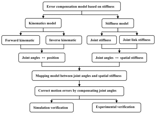
Figure 1.
Schematic of the proposed method.
2. Kinematics Model for a 6-DOF Robotic Manipulator
The improved DH method [21] was used to establish the connecting rod coordinate system of the manipulator, and the kinematics model was used to obtain the analytic solution of the forward and inverse kinematics of the manipulator, by which the motion posture of the manipulator could be obtained. This method was also the foundation for solving the stiffness matrix.
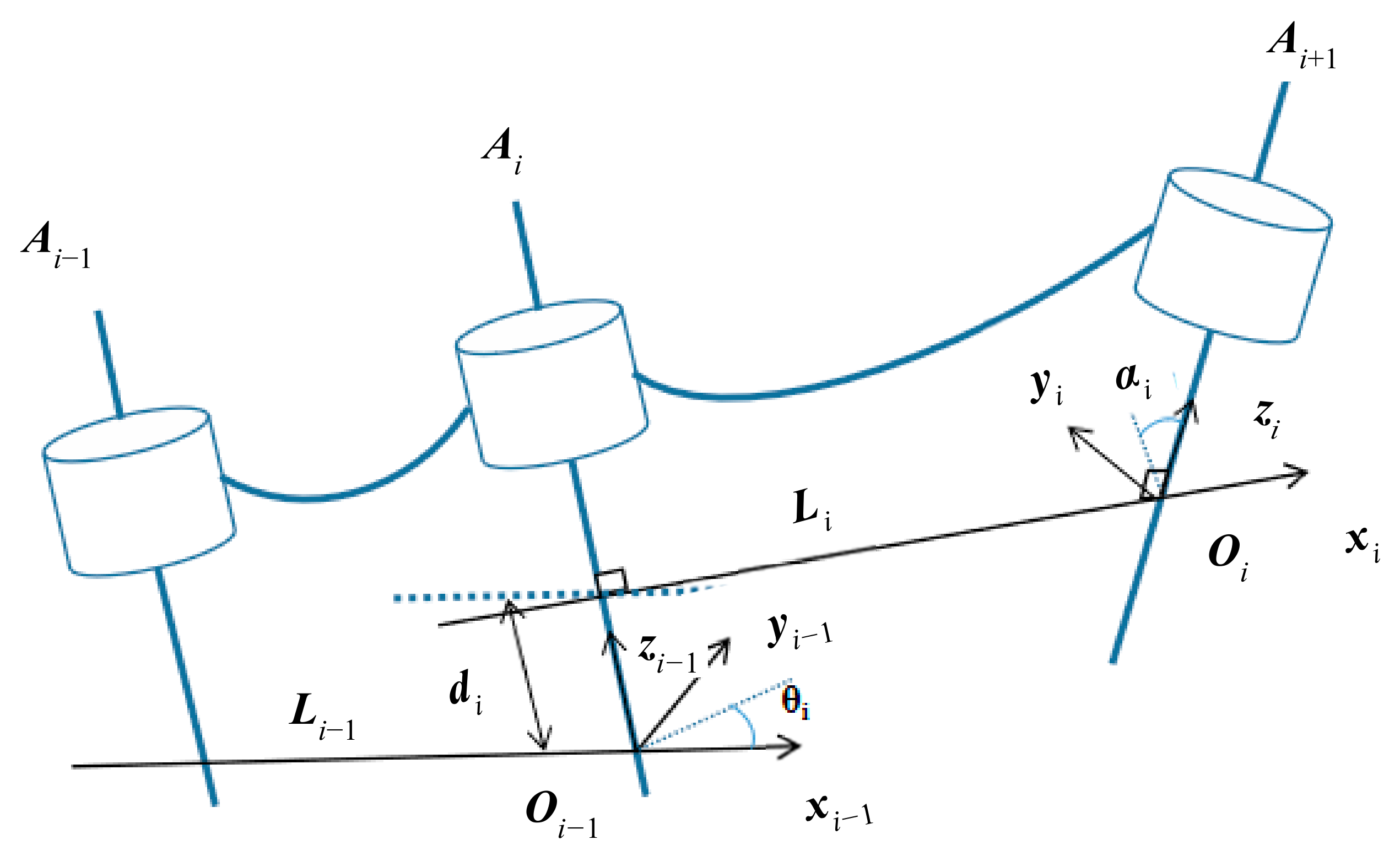
For the forward kinematics model, the connecting rod coordinate system of a 6-DOF manipulator (Figure 2a) was established as follows: first, the position of the base coordinate system and the initial position and attitude angles of the end were determined. Second, the improved DH method was adopted to establish the coordinate system of the base and each joint, and the forward kinematics solution model was utilized to calculate the point-to-point (PTP) trajectory. The established coordinate system is shown in Figure 2b. Figure 3 shows one of the connecting rod coordinate systems.
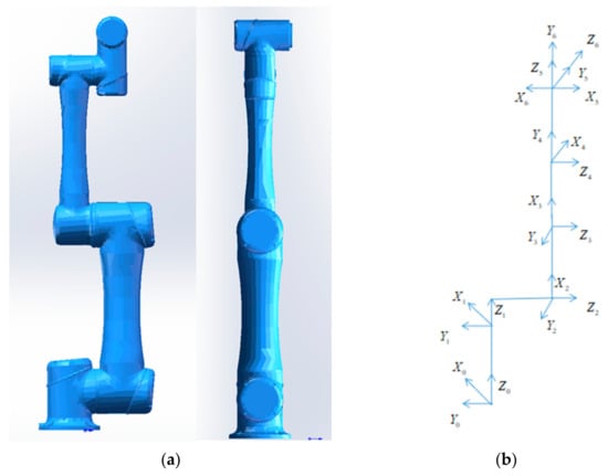
Figure 2.
(a) 6-DOF manipulator model and (b) connecting rod coordinate system.
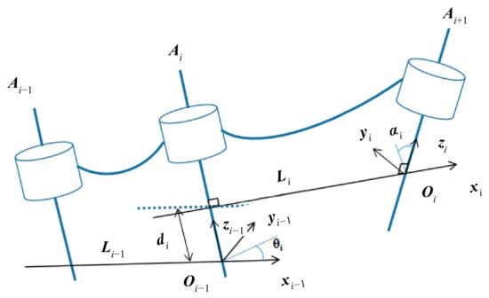
Figure 3.
Connecting rod coordinate system.
From Figure 3, the homogeneous transformation matrix of the linkage can be obtained as follows:
where Rot and Trans represent the rotation matrix and translation matrix, respectively, and i represents the number of joints., , , and represent the angle, connecting rod torsion angles, connecting link length, and connecting rod offset, respectively, of joint i.
The end posture (including position and attitude) of the 6-DOF manipulator (4 × 4 matrix) was calculated as follows:
To solve the angles of the six joints from the space posture inversion of the manipulator and pave the way for the subsequent compensation model, the inverse kinematics of the manipulator need to be solved. The angles of the six joints can be obtained by solving eight inverse kinematics solutions with the improved algebraic method, which will be explained in detail in Section 4.
3. Trajectory Compensation Based on Stiffness Modeling
To solve the relationship between the stiffness and the space position error caused by it, first, the Jacobian matrix of the manipulator was solved by using the vector product method. Second, the stiffness matrix of the manipulator was solved with the given generalized force and manipulator parameters. Last, the mapping model of the six angles of the manipulator and the errors caused by the joint stiffness of the manipulator were established.
3.1. Construction of the Jacobian Matrix
The Jacobian matrix was mainly employed in the velocity/static mapping between the manipulator end and the joint. In essence, it is a partial differential matrix. The number of rows represents the free degree of space (X, Y, Z, α, β, and γ), and the number of columns represents the number of physical rotational axes of the robot. The Jacobian matrix J(q) can be regarded as the linear relationship between the joint velocity and the manipulator space velocity or the linear relationship between the joint variable and the end deformation, which can be obtained as follows:
where v represents the linear velocity of the end of the manipulator and ω represents the angular velocity of the end. Therefore, the linear velocity v and angular velocity ω of the robotic end can be expressed in terms of the joint velocity qi:
where Jli and Jai represent the linear velocity and angular velocity, respectively, of the end caused by the unit joint velocity of joint i.
The Jacobian matrix connects the joint velocity with the end Cartesian velocity:
where v and w are the linear velocity and angular velocity, respectively, and q is the joint velocity vector. Since velocity can be taken as the differential motion per unit time, the Jacobian matrix can also be considered as the transformation matrix between the differential motion in joint space and the differential motion in operating space, namely,
where d and δ are the differential movement and rotation at the end, respectively, and dq is the joint differential motion vector.
For joint i, the angular velocity ω at the end is
where qi represents the angle of the joint, zi is the representation of the z-axis unit vector of frame {i} in the base frame {0}, n is the number of joints of the manipulator, and ε is a coefficient, which will be explained in Equation (8).
The linear velocity v generated by joint i at the end is
where ; if joint i is revolute, ε = 0, and if joint i is prismatic, ε = 1 (the joints of the manipulator in this paper are all revolute). represents the position vector of the end origin relative to the coordinate system {i} in the base system {0}, namely,
Therefore, for joint i of the rotation, the i-th column of the Jacobian matrix is
where represents the rotation matrix of joint 0 transformed to joint i.
The Jacobian matrix of the manipulator can be calculated according to the formulas in this section.
3.2. Flexibility Matrix
External loading will cause deformation of the manipulator due to the lack of stiffness. Joint deformation basically accounts for a large proportion of deformations, while other deformations account for a very small proportion.
The spring coefficient Kqi was assumed to represent the stiffness of the entire drive system:
where τi is the joint torque, dqi is the additional deformation caused by the action of joint variables qi from τi, and the total relation is
where represents the matrix whose diagonal elements are .
Based on the error derived from the differential motion relation and Jacobian matrix of the forces, the following relation can be obtained:
The inverse of is , which is often referred to as joint flexibility.
Let the end flexibility matrix be , then
Equation (15) is used to represent the relationship between the error (or ) of the working space and the generalized force F, which can be expressed as
where D is proportional to , so the deformation at the end of the manipulator will change as the Jacobian matrix changes.
3.3. Error Compensation Model for a 6-DOF Manipulator
3.3.1. Joint Stiffness
Assuming that the force on the end of the arm is , then
where and represent three-dimensional force vectors and three-dimensional moment vectors, respectively.
The deformation at the end due to the external force is X:
where and represent translational deformation and rotational deformation, respectively.
When the force is within a certain range, the relationship between the force and the deformation satisfies a linear relationship, i.e., following Hooke’s law:
The stiffness matrix or flexibility matrix of the robot reflects the linear relationship between the end force F and the deformation X and varies with the change in shape and position. From the elements in the stiffness matrix, it can be seen that the force in a certain direction not only causes deformation in a certain direction but also causes deformation in other directions.
The stiffness matrix can be obtained by combining the Jacobian matrix calculated in the previous section with the stiffness calculation formula:
The inverse matrix of C−1 is C, which is referred to as the flexibility matrix.
3.3.2. Manipulator Arm Link Stiffness
For the joint link i, its stiffness can be expressed as
where and represent translational stiffness and rotational stiffness, respectively. In addition, the force f on the joint link i can be expressed as
where , , and are the forces in the X direction, Y direction, and Z direction, respectively, and , , and represent the torque on the link. The force and torque transmitted from the end of the manipulator to arm link i can be calculated by the following formulas:
,, , and , can be obtained from Equation (2) when the generalized forces and generalized stiffness at the end of the manipulator are known; the generalized displacement deformation of the manipulator arm link is
where , , , , and .
The displacement deformation δi can be obtained by the following material mechanics formula, which is hard to apply to the quantitative measurement of the positioning error of the manipulator end, and will be replaced by the result of the finite element analysis.
Thus, the error caused by the stiffness of the total joint arm link can be calculated:
According to the deformation caused by the stiffness of the manipulator link and the deformation caused by the stiffness of the joint, the total deformation δ of the industrial robot can be obtained:
The generalized force F on the operating end of the manipulator is
where , and are the forces in the X direction, Y direction, and Z direction, respectively, and , and , respectively, represent the torque on the link. is the generalized force exerted on the end, is the generalized deformation of the end, and then the total space stiffness of the manipulator can be obtained:
3.3.3. Motion Error Compensation by Correcting Joint Angle
According to the stiffness formula derived previously, when the stiffness and the generalized force F at the end are known, the end error Δδ can be calculated:
When there is no external load on the robot, the joint angle is regarded as the theoretical joint angle , and its end position is the theoretical position . When the robot is under an external load, its joint angle and end position will deviate due to its stiffness, the joint angle is the actual value , and the end position is the actual position . The deformation at the end of the robot subjected to external load causes the error of the end position. In this paper, the error is compensated by correcting the joint angle by .
4. Simulation Studies for a 6-DOF Manipulator
As described in this section, a 6-DOF manipulator was taken as an example to carry out the simulation studies. First, the forward and inverse kinematics model was established, and then the stiffness and stress of the joint were analyzed to determine the influence of the joint stiffness on the end position error. Second, the stiffness variation of the manipulator in its motion space was determined. Last, the angular stiffness space position error model was established to simulate and calculate the stiffness and error changes in the motion trajectory.
4.1. Solving Kinematics Model
Inverse kinematics were utilized for the establishment of the joint angle compensation model, so this section solves the inverse kinematics for the 6-DOF manipulator. The DH parameters for the manipulator are listed in Table 1.

Table 1.
DH parameters for the 6-DOF robotic manipulator.
According to the forward model in Section 2 and combined with the DH parameters of the 6-DOF manipulator, the following expressions can be obtained based on Equation (2):
where
The inverse model for the manipulator can be solved by the following steps.
To obtain , transform the matrix of both sides of Equation (34):
The values in row 3 and column 4 are equal, and is obtained:
where and .
Using row 3, column 3 on both sides of the equation corresponds to the same thing, and then is obtained:
The third row and the first column on both sides of the equation are equal, and is obtained:
where .
To obtain , transform the matrix of both sides of Equation (3):
According to the left and right sides of row 1 of this equation, column 4 corresponds to the same thing; row 2, column 4 corresponds to the same thing; and , , and are obtained:
where .
Based on these equations, the corresponding inverse kinematics solutions of eight groups () can be obtained.
4.2. Errors Caused by Connecting Rod Deformation
A mechanical analysis model of the manipulator was established, and a stress analysis was carried out to compensate for the errors caused by connecting rod deformation. To facilitate the stress analysis of the manipulator, the model of the manipulator was simplified and constructed in ANSYS software, and the basic configuration and rigid body characteristics of the manipulator with six degrees of freedom were retained. The ‘material’ was set as ‘structural steel’ and the ‘mesh’ was set as ‘medium’. Under the experimental conditions, it was difficult to keep the generalized force constant on the manipulator arm, so the direction of the generalized force was set as straight down, which is also helpful to design experiments. Figure 4 shows the deformation of the manipulator when the manipulator arm was in a posture with different loads of 0 N, 10 N, and 20 N. The maximum displacement of the manipulator itself was basically maintained at approximately 0.03 mm. However, it can also be seen that errors caused by the stiffness of the connecting rod of the manipulator do exist and will affect the positioning accuracy of its end. Considering that the stiffness model of the joint link was very difficult to calculate, a finite element analysis was carried out for the different postures of the manipulator to better compensate for the error. The displacement results of the finite element analysis were added to the final error compensation model as the additional generalized errors of the manipulator.
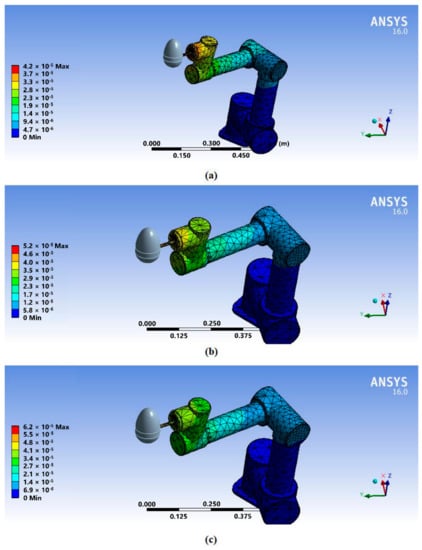
Figure 4.
Deformation of the manipulator under different loads in the Z direction: (a) 0 N, (b) 10 N, and (c) 20 N.
4.3. Flexibility Elements in Six Directions
The joint stiffness data were obtained based on the joint module specification and relevant parameters that are commonly employed in harmonic reducers [22]: (unit: N·mm/rad), where represents the matrix whose diagonal elements are . The parameter K is defined by
where and are the load torque and elastic deformation angle, respectively, of the harmonic reducer.
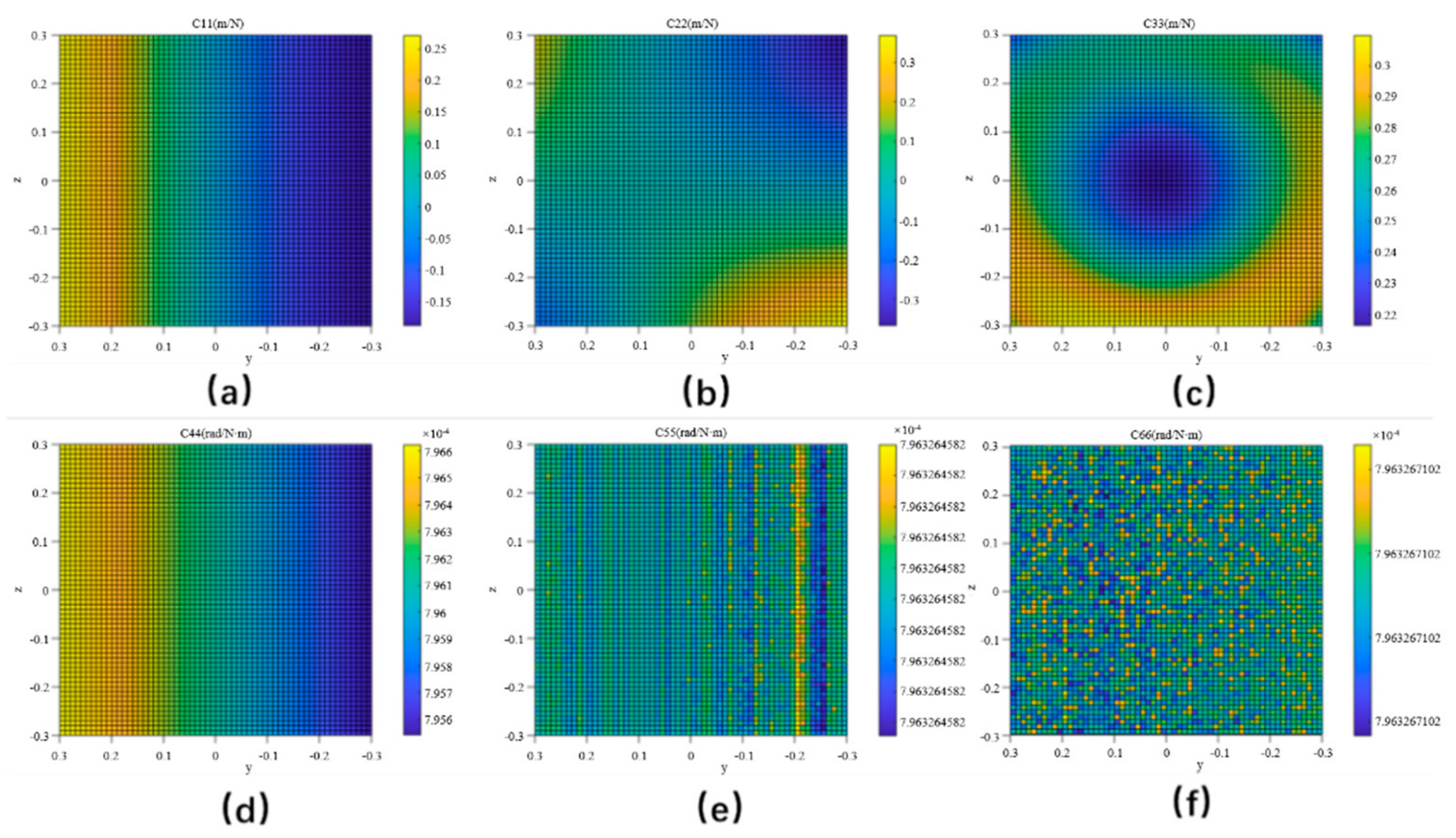
From Equation (15), the stiffness matrix C can be obtained. However, stiffness reflects the force caused by the change in the unit displacement, while flexibility reflects the displacement caused by the unit force. The research focus of this paper is the displacement error caused by insufficient stiffness. The derivation of the flexibility matrix C with the diagonal elements shows that the elements represent the moving deformation caused by unit force in the X, Y, and Z directions, while represent the rotational deformation caused by the unit torque in the X, Y, and Z directions. When X = 0.3, Y and Z are at (−0.3, 0.3) (unit: m), the end attitude angles are (−1.57, 0, 1.57) (unit: rad), the stiffness matrix can be solved, and the flexibility plane of . is as shown in Figure 5
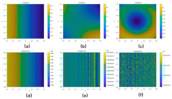
Figure 5.
Flexibility matrix elements plane: (a)
(b) , (c) , (d) , (e) , and (f) .
Figure 5 shows the displacement changes at the end of the manipulator in the X, Y, and Z directions and the attitude angles (α, β, and γ), which indicate that the stiffness is different when the manipulator moves in space. Flexibility reflects the displacement under a force. Figure 5a shows that when the manipulator moved from −0.3 m to 0.3 m along the Y axis, the error of the end in the X direction caused by insufficient stiffness decreased. However, when moving along the Z axis, it did not change greatly, which may be because the manipulator was in the reasonable working range of the Z axis. Figure 5b shows that when the manipulator moved from y = −0.3 m to y = 0.3 m, when the Z coordinate was large, the flexibility in the Y direction decreased and then increased. When the Z coordinate was smaller, the flexibility in the Y direction increased. When the Z coordinate was near 0, the flexibility was basically unchanged at approximately 0.1 m/N. Figure 5c shows that the flexibility of the end of the manipulator in the Z direction presented a Newtonian annular variation in the motion plane. Figure 5f show the variation in the angular displacement compliance at the end of the manipulator.
The simulation results in this section indicate that the stiffness of the manipulator at each point in space is different, the change regularity is difficult to predict, and the errors caused by it are constantly changing, for which it is necessary to compensate the errors for better accuracy of the end positioning. In the following sections, the joint angle is compensated to verify the compensation effect by the simulation and experiments.
4.4. Simulations of Error and Stiffness in PTP Trajectory
Given the generalized force (N), the total end stiffness K and total generalized deviation were obtained in the point-to-point trajectory. , , and are commonly employed to measure the positional deviation, which is the deviation in the end position in the X direction, Y direction, and Z direction, respectively.
The motion trajectory of the manipulator was set from point (207, 444, 631) to point (−137, 69, 241) (including 40 points). The stiffness and position error in the translation direction of X, Y, and Z in the process of motion were obtained by using the derived stiffness formulas, as shown in Figure 6 and Figure 7.
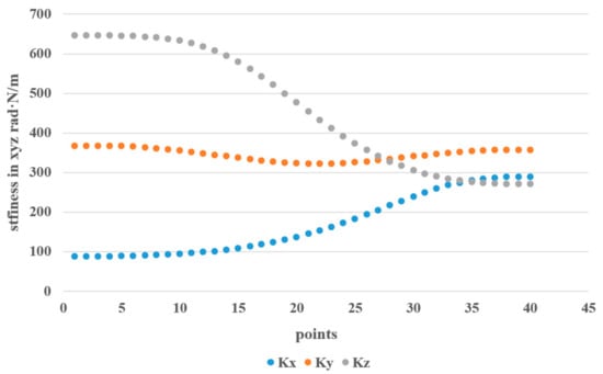
Figure 6.
Stiffness changes in the translation direction of X, Y, and Z.
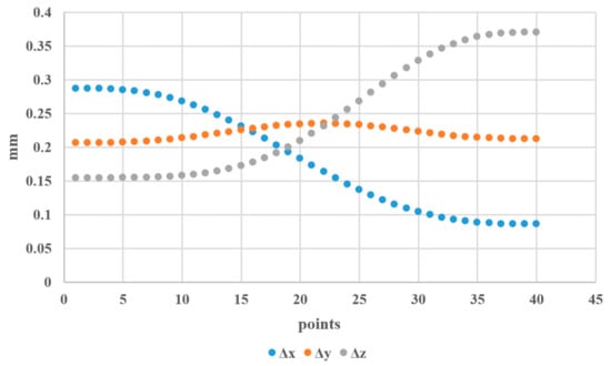
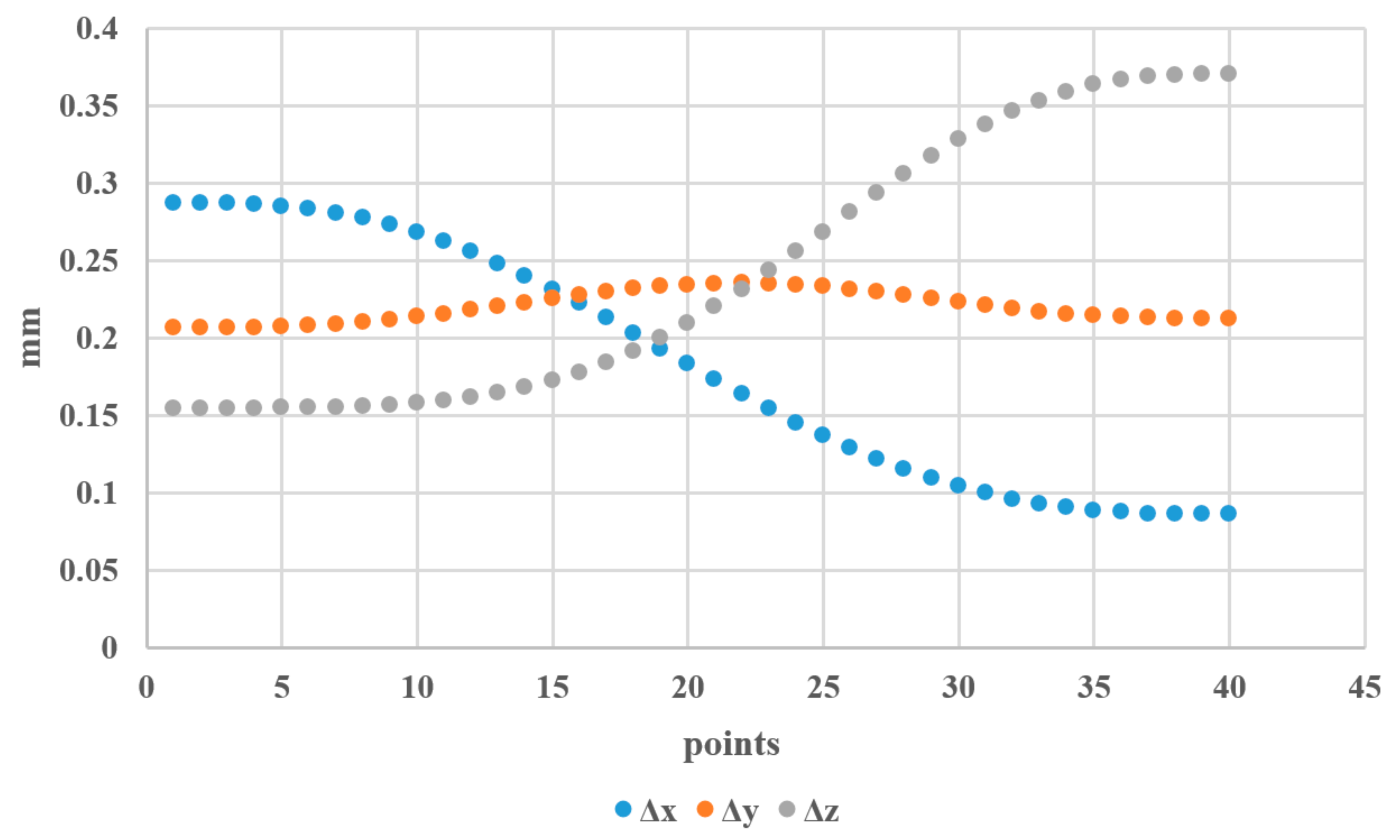
Figure 7.
Position errors in the X, Y, and Z translation directions.
With the movement of the manipulator, the stiffness in the X, Y, and Z translational directions will also change. The stiffness in the Y direction was basically unchanged at approximately 350 rad·N/m, and its error basically fluctuated at approximately 0.2 mm. During the movement of the manipulator arm, the stiffness in the Z direction decreased from 640 to 270 rad·N/m, and the corresponding position error increased from 0.15 mm to 0.37 mm. When the stiffness in the X direction increased from 100 to 280 rad·N/m, the corresponding error decreased.
4.5. Trajectory Error Compensation
The PTP trajectory of the previous part was compensated, and the compensation angle of joint angle was calculated by using Equations (38)–(42), as shown in Figure 8. The space coordinate errors before the error correction are shown in Figure 9.
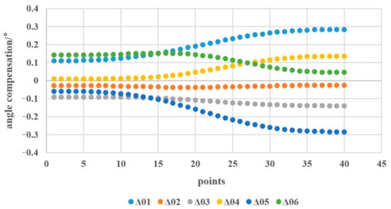
Figure 8.
Compensated angles for joint angle .
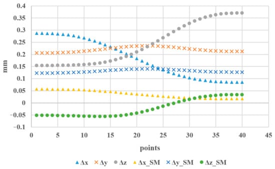
Figure 9.
Spatial coordinate errors before the error correction.
In Figure 9, , , and represent the position error in the X direction, Y direction, and Z direction, respectively, before the compensation of the joint angles, while , , and represent the corresponding position errors after angle compensation. The simulation results show that the position errors of the manipulator end were reduced in the X, Y, and Z directions.
5. Experimental Studies
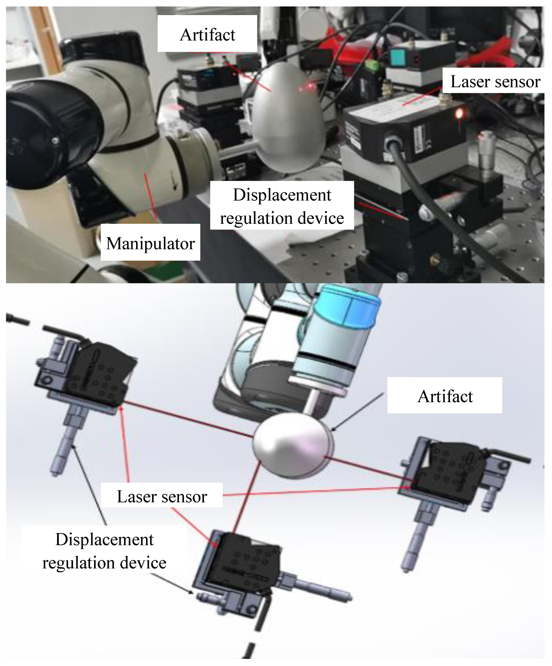
In the experimental studies, a 6-DOF robotic manipulator (named AR5 from Asage-Robots Ltd., China) was taken as the objective. The end position of the manipulator was measured by an artifact installed at the end, which was measured by three displacement laser sensors (Keyence LK-G500) [23]. The measurement system is shown in Figure 10.
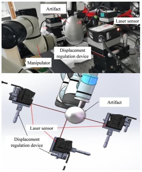
Figure 10.
End position measurement system for a 6-DOF robotic manipulator.
Based on the previously established joint angle-stiffness-spatial position error model, a series of experiments were carried out to verify the effectiveness of the model. The experiments included two parts. In the first part, the space position of the manipulator was measured under the same trajectory but with different loads. Six random points were selected from the measurement range of the manipulator and the measurement system. The spatial position of each point was measured under different loads at the end of the manipulator to verify the regularity of the joint angle-stiffness-spatial position model. In the second part, an additional error compensation experiment was carried out, and the spatial error of the manipulator end was compared between the simulation results and the measured results.
5.1. Position Error under Different Loads
Generally, the repeat positioning accuracy or position precision was high for the robotic manipulator. Therefore, for the same trajectory, the initial point and end point can be considered the same without the end load, and the difference between the spatial position of the initial point and that of the final point under load was measured to verify whether it conformed to the validity of the proposed stiffness model.
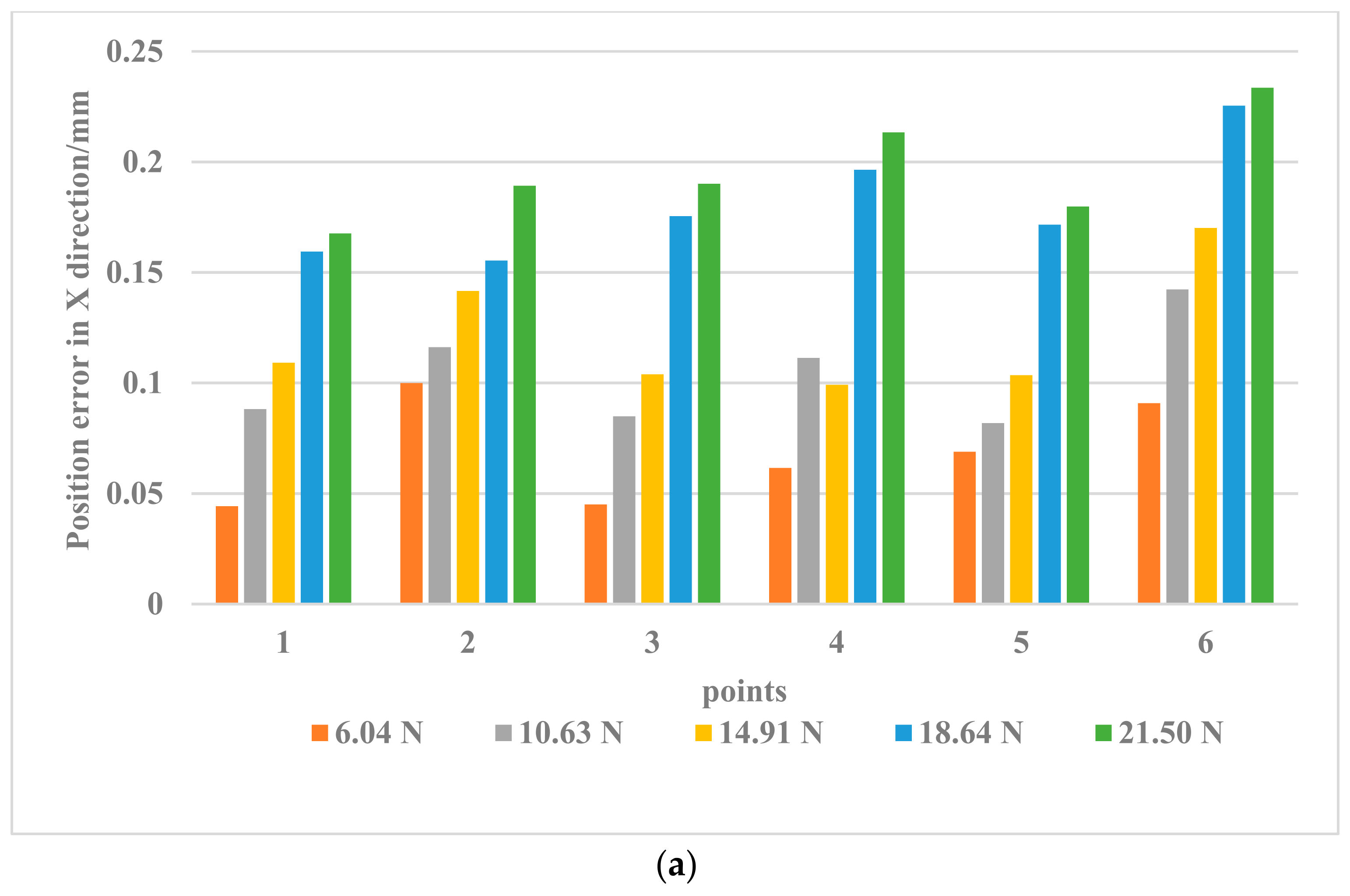
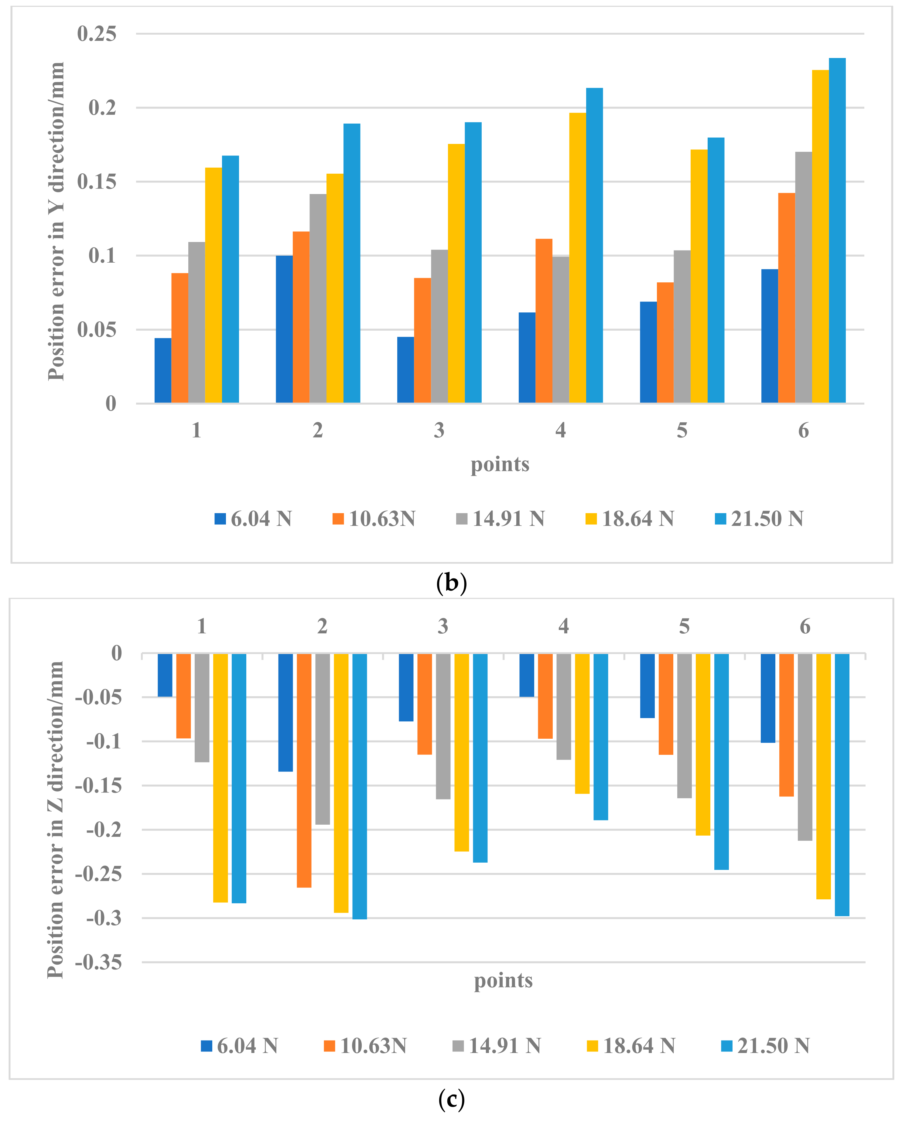
The posture of the manipulator at the initial point was set to (253.419 mm, 6.866 mm, 432.48 mm, 90.26°, 84.23°, 93.55°), in which the first three parameters are the Cartesian coordinates of the end of the manipulator, and the last three parameters are the attitude angles of the end of the manipulator. Loads of 0 N, 6.04 N, 10.63 N, 14.91 N, 18.64 N, and 21.50 N were added to the end of the manipulator (the force was applied in a downward direction). In each load state, the initial position was repeatedly positioned at the initial point several times to ensure the stability of the initial coordinates, the complete track was followed coherently, and the spatial position of each static track point was recorded. According to the previous stress analysis, this experiment put the applied load on the end of the manipulator. The force at the end of the arm was distributed differently in the X, Y, and Z directions, resulting in corresponding error changes in different directions, as shown in Figure 11.
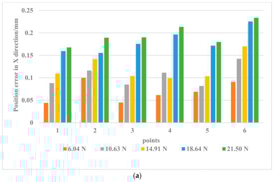
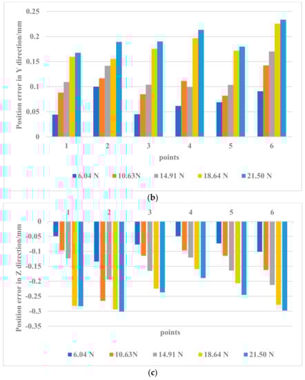
Figure 11.
Position error in (a) X, (b) Y, (c) Z direction under different loads.
The changes in the position errors when the load is 18.64 N and 21.50 N in Figure 11a–c show that when the load force at the end increased to a certain extent, the errors caused by the load changes gradually decreased; that is, the load force is not a linear factor for the increase in errors at this time. The results in the figures show that when the manipulator was at different points in space (at different postures), the position and pose of the manipulator had a more important role in the errors caused by stiffness. The position error caused by a small force was sometimes greater than that caused by a larger force, for example, a mutation of the position error appeared when the position error at 10.63 N exceeded the error caused by 14.91 N. According to the variation characteristics of most position errors in Figure 11, this sudden change may have been caused by additional errors in the measurement process (possibly the drift of the laser sensor).
The experimental results in this section show that when the load force at the end of the manipulator increased to a certain extent, its influence on the position error was gradually weakened, while the influence of the manipulator attitude always existed. Under the same conditions, the influence of the joint angle had a greater influence on the error than other factors.
5.2. Compensation of Position Error under Different Loads
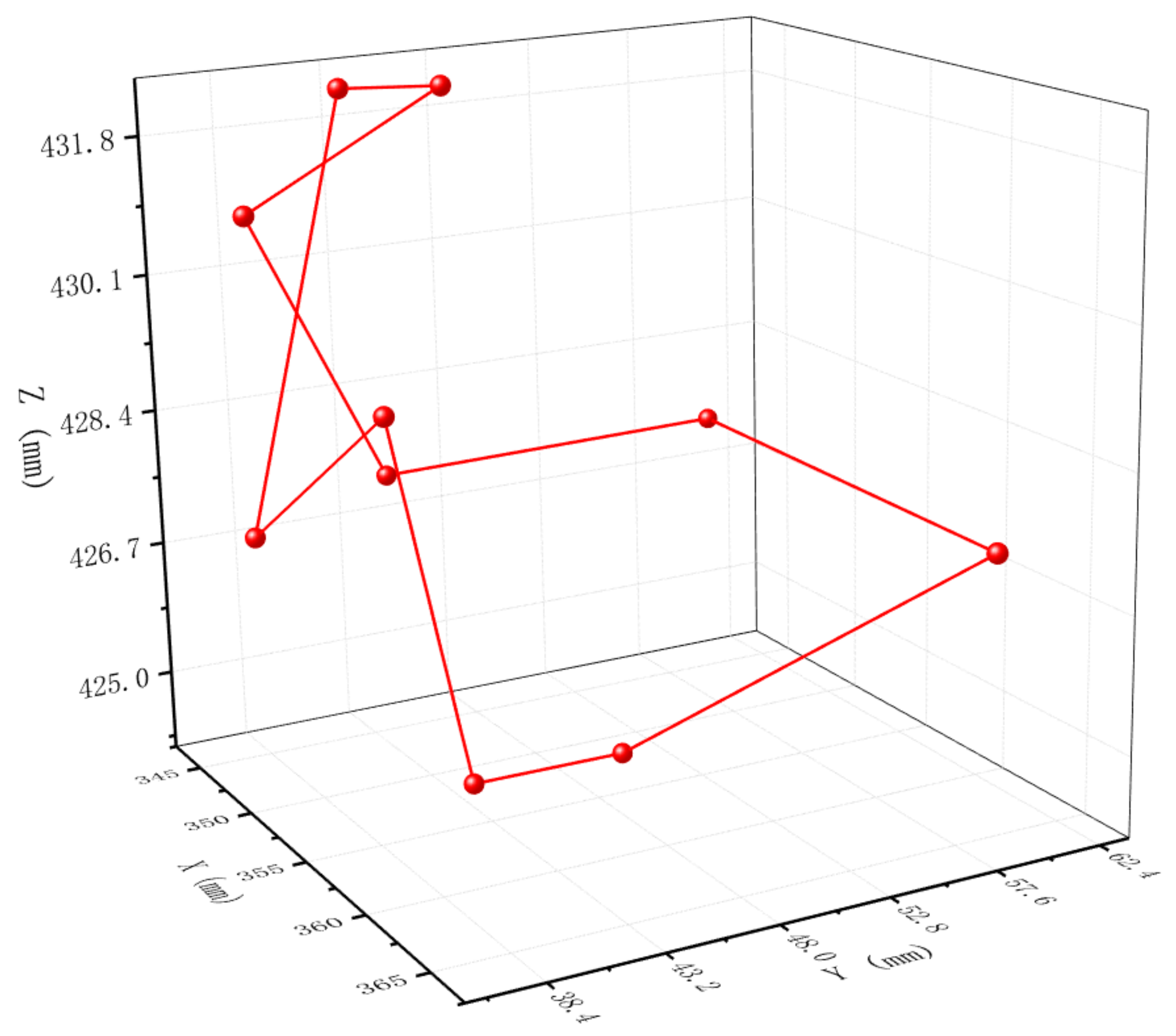
In this section, the end position of the manipulator arm under two conditions with a load of 10.6 N and 18.04 N was measured. Since the positioning precision of the manipulator at a load of 0 N load was much higher than the absolute positioning accuracy, the end position of the manipulator at a load of 0 N was considered the reference. A total of 11 points were randomly selected in the Cartesian coordinate space of the manipulator in the experiment, as shown in Figure 12.
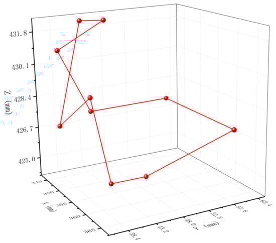
Figure 12.
Selected 11-point trajectory.
According to the error-joint angle model (Equation (14)),
where .
According to the Jacobian construction method in Section 3.1, can be obtained:
where the homogeneous transformation parameters of joint : ,,, , , , , and can be obtained according to Equation (46):
where is the homogeneous transformation matrix for joint .
can be obtained from Section 4.3, and F is the six-dimensional generalized force applied at the end of the manipulator, as shown in Equation (28).
The compensated angle ∆q can be obtained as
The first point and the last point coincide, which is not only for the verification of the repetition accuracy of the same point but also for the observation of the position error of joint stiffness superposition. Table 2 and Table 3 show the compensation angles of the six joint angles under a load of 10.6 N and 18.0 N, respectively. Figure 13 shows the position errors before and after compensation, where X_error, Y_error, and Z_error represent the position errors in the X direction, Y direction, and Z direction, respectively, and X_SM, Y_SM, and Z_SM represent the position errors after compensation based on the stiffness model in the X direction, Y direction, and Z direction, respectively.
Table 2.
Compensated joint angles ∆q (under 10.6 N).
Table 3.
Compensated joint angles ∆q (under 18.0 N).
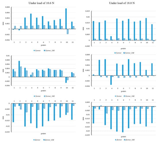
Figure 13.
Position error before and after compensation under different loads.
As shown in Figure 13, the position error in the X and Y directions was generally less than 0.01 mm because the external force was mainly applied in the Z direction. After the joint angles were compensated, the displacement errors in these two directions were reduced to less than 0.005 mm. In the Z direction, the maximum error reached −0.3 mm, which was basically reduced to less than 0.01 mm, and the minimum value was only 0.0015 mm after compensation. The compensation effect of the displacement errors in the X, Y, and Z directions reached 95.2%, 98.7%, and 96.2%, respectively. The experimental results of this paper indicate that the error compensation method by the stiffness model based on joint stiffness and joint link stiffness is effective, which is significant for improving the spatial positioning accuracy of 6-DOF manipulator ends.
Researchers should discuss the results and how they can be interpreted from the perspective of previous studies and of the working hypotheses. The findings and their implications should be discussed in the broadest context possible. Future research directions may also be highlighted.
This section is not mandatory but can be added to the manuscript if the discussion is unusually long or complex.
6. Concluding Remarks
A new method of motion error modeling and compensation for robotic manipulators was proposed in this paper. Forward and inverse kinematics models for a 6-DOF robotic manipulator were established. The Jacobian matrix and stiffness matrix were calculated based on the parameters of the joint modules. The mapping model of the 6 joint angles, generalized force at the end, and spatial stiffness was built. In the case that generalized force is known, the joint stiffness can be simulated for the motion errors of the manipulator end. Based on the simulation results, the error compensation method based on joint angles was established. In the simulation and experimental studies, a reasonable compensation effect was obtained. The compensation effect of the displacement errors in the X direction, Y direction, and Z direction reached 95.2%, 98.7%, and 96.2%, respectively. The findings are useful in posture selection and joint angle compensation for maintaining the optimal stiffness of the manipulator. The research work is also helpful for enhancing the overall stiffness and reducing the motion errors of the robotic manipulator, and hence, improving the working performance and accuracy of the manipulator. This improvement will extend the application of the robotic manipulator in precision machining and measurement.
However, in this study, the speed of the manipulator was relatively slow during movement; therefore, the influence of static stiffness was mainly considered without considering the factor of speed. In future research, motion velocity will be considered in the compensation model to establish a more comprehensive relationship among the magnitude of velocity, acceleration, and compensation angle to further improve the error compensation effect and position accuracy during the movement of the manipulator.
Author Contributions
Writing—original draft preparation, experiments, and algorithms, X.H.; conceptualization, writing—review and editing, supervision, and funding acquisition, L.K.; writing—review and editing, G.D. All authors have read and agreed to the published version of the manuscript.
Funding
National Key R&D Program of China (No. 2017YFA0701200), National Natural Science Foundation of China (No.52075100), and Shanghai Science and Technology Committee Innovation Grant (No. 19ZR1404600).
Institutional Review Board Statement
Not applicable.
Informed Consent Statement
Not applicable.
Data Availability Statement
Not applicable.
Conflicts of Interest
The authors declare no conflict of interest.
References
- Cai, Z.X.; Xie, B. Robotics, 3rd ed.; Tsinghua University Press: Beijing, China, 2015; pp. 1–12. [Google Scholar]
- Wang, B.J.; Teng, S.F. Industrial Robot; Huazhong University of Science and Technology Press: Wuhan, China, 2015; pp. 8–15. [Google Scholar]
- Tan, H.H. Modeling and Elastic Dynamics Analysis of the Overall Stiffness of 6R Industrial Robots; Huazhong University of Science and Technology: Wuhan, China, 2013. [Google Scholar]
- Liu, W.Z. Stiffness Modeling and Application Research of 6R Industrial Robot; Lanzhou University of Technology: Lanzhou, China, 2014. [Google Scholar]
- Dumas, C.; Caro, S.; Gamier, S.; Furet, B. Joint stiffness identification of six-revolute industrial serial robots. Robot. Comput.-Integr. Manuf. 2011, 27, 881–888. [Google Scholar] [CrossRef] [Green Version]
- Lehmann, C.; Olofsson, B.; Nilsson, K.; Halbauer, N.; Haage, M.; Robertsson, A.; Sornmo, O.; Berger, U. Robot Joint Modeling and Parameter Identification Using the Clamping Method. IFAC Proc. Vol. 2013, 46, 813–818. [Google Scholar] [CrossRef]
- Ailon, A.; Michael, I.G. Stability analysis of a rigid robot with output-based controller and time delay. Syst. Control Lett. 2000, 40, 31–35. [Google Scholar] [CrossRef]
- Klimchik, A.; Furet, B.; Caro, S.; Pashkevich, A. Identification of the manipulator stiffness model parameters in industrial environment. Mech. Mach. Theory 2015, 90, 1–22. [Google Scholar] [CrossRef] [Green Version]
- Wang, R.C.; Zhang, W.M.; Sun, J.B. Influence of offset stiffness matrix on robot milling. Mach. Manuf. 2018, 8, 80–83. [Google Scholar]
- Lin, G.L.; Lin, C.C.; Chen, B.C.; Soong, T.T. Vibration control performance of tuned mass dampers with resettable variable stiffness. Eng. Struct. 2015, 83, 183–197. [Google Scholar] [CrossRef]
- Ye, Y.J.; Lin, Y.F.; Cai, D.W. Spinal motion control based on 6-DOF robotic arm. Med. Biomech. 2019, 4, 1–5. [Google Scholar]
- Geng, S.N.; Wang, Y.Y. Design and control of variable stiffness continuous manipulator. Acta Astronaut. Sin. 2018, 39, 1391–1400. [Google Scholar]
- Liao, Z.Y.; Li, Z.R.; Xie, H.L.; Wang, Q.H.; Zhou, X.F. Region-based toolpath generation for robotic milling of freeform surfaces with stiffness optimization. Robot. Comput.-Integr. Manuf. 2020, 64, 101953. [Google Scholar] [CrossRef]
- Raoofian, A.; Taghvaeipour, A.; Kamali, A. On the stiffness analysis of robotic manipulators and calculation of stiffness indices. Mech. Mach. Theory 2018, 130, 382–402. [Google Scholar] [CrossRef]
- Jhan, Z.Y.; Lee, C.H. Adaptive Impedance Force Controller Design for Robot Manipulator including Actuator Dynamics. Int. J. Fuzzy Syst. 2017, 19, 1739–1749. [Google Scholar] [CrossRef]
- Han, Y.; Courteille, E.; Gouttefarde, M.; Herve, P.E. Vibration analysis of cable-driven parallel robots based on the dynamic stiffness matrix method. J. Sound Vib. 2017, 394, 527–544. [Google Scholar]
- Zhang, Z.L. Research on Dynamic Characteristics of Space Manipulator Based on Active Control of Arm Stiffness; Beijing Technology and Business University: Beijing, China, 2020. [Google Scholar]
- Chen, X.J.; Gulinar, Z.N.; Xue, Z.; Li, D.; Ban, Z.; Ren, G. Calibration Algorithm and Experimental Research of Cooperative Robot Based on Laser Tracker. Acta Metrol. Sin. 2021, 42, 552–557. [Google Scholar]
- Ren, T.; Luo, M.Z.; Zhang, J.L. Kinematics Error Model and Calibration Algorithm of Cooperative Robot. Mach. Build. Autom. 2021, 50, 163–167. [Google Scholar]
- Tian, J.F. Calibration Method of Modular Cooperative Robot Considering Joint Stiffness; Tianjin University: Tianjin, China, 2017. [Google Scholar]
- Ghost, H.K. Introduction to robotics: Mechanics and Control (second edition). J. Mater. Process. Technol. 1991, 25, 239–240. [Google Scholar]
- ASAGE Robots. Available online: http://www.asage-robots.com/industry.html (accessed on 1 October 2021).
- Kong, L.B.; Yu, Y. Pose Measuring and Industrial Robot Kinematics Model Correcting Method for Industrial Robot. China Patent CN201911341888.4, 10 April 2020. [Google Scholar]


Publisher’s Note: MDPI stays neutral with regard to jurisdictional claims in published maps and institutional affiliations. |
© 2021 by the authors. Licensee MDPI, Basel, Switzerland. This article is an open access article distributed under the terms and conditions of the Creative Commons Attribution (CC BY) license (https://creativecommons.org/licenses/by/4.0/).