
Carbon Dioxide Decomposition by a Parallel-Plate Plasma Reactor: Experiments and 2-D Modelling

 ,
,  ,
,  ,
,
Abstract
:Featured Application
Abstract
1. Introduction
2. Materials and Methods
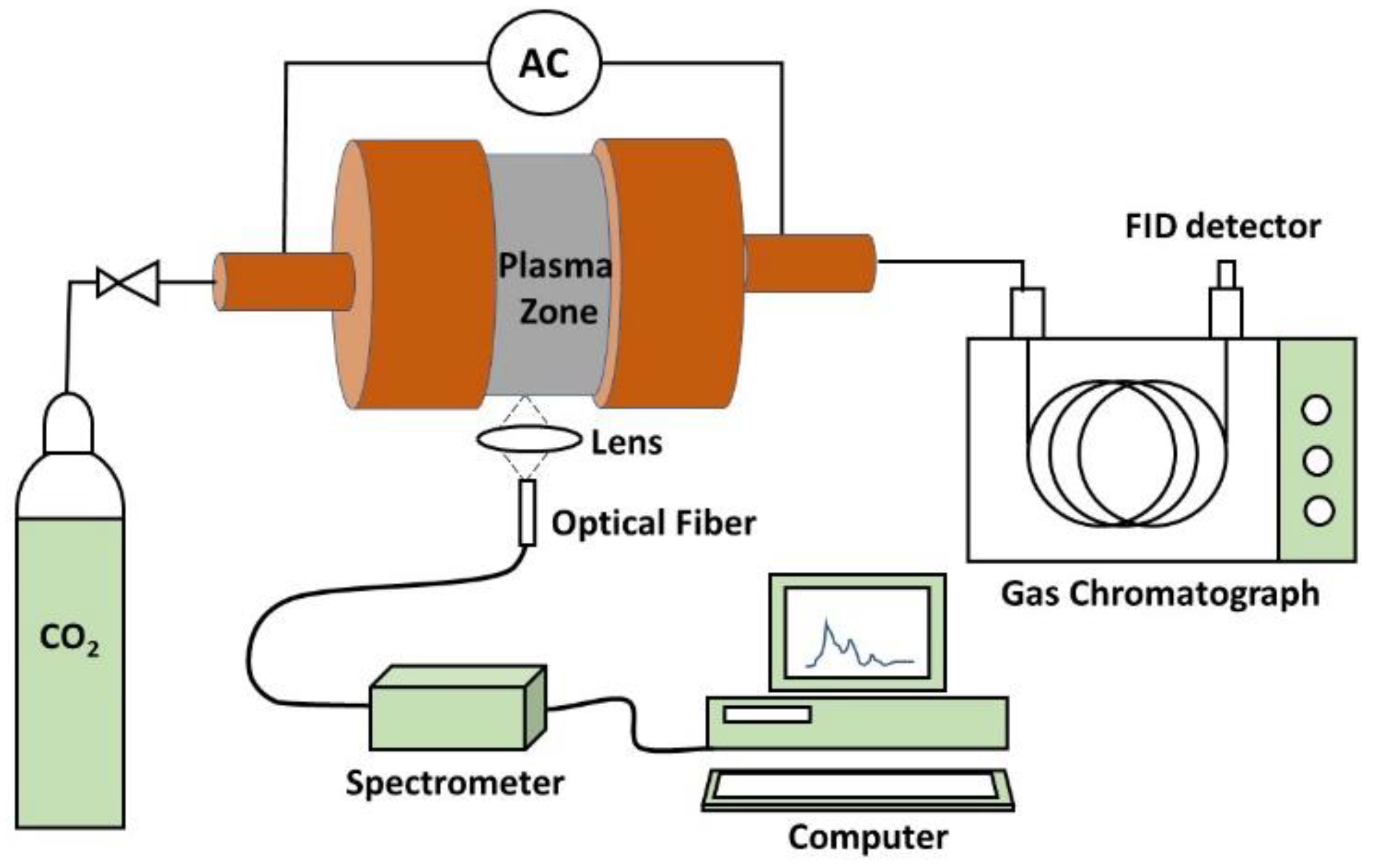
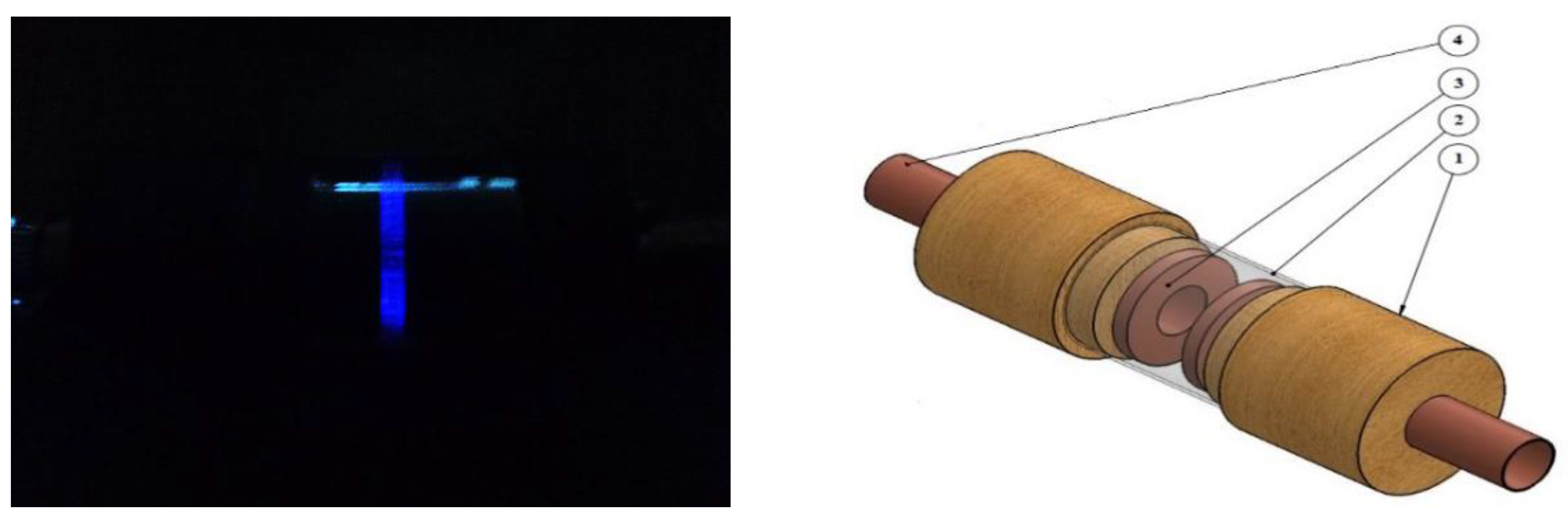
2.1. Experimental Set-Up
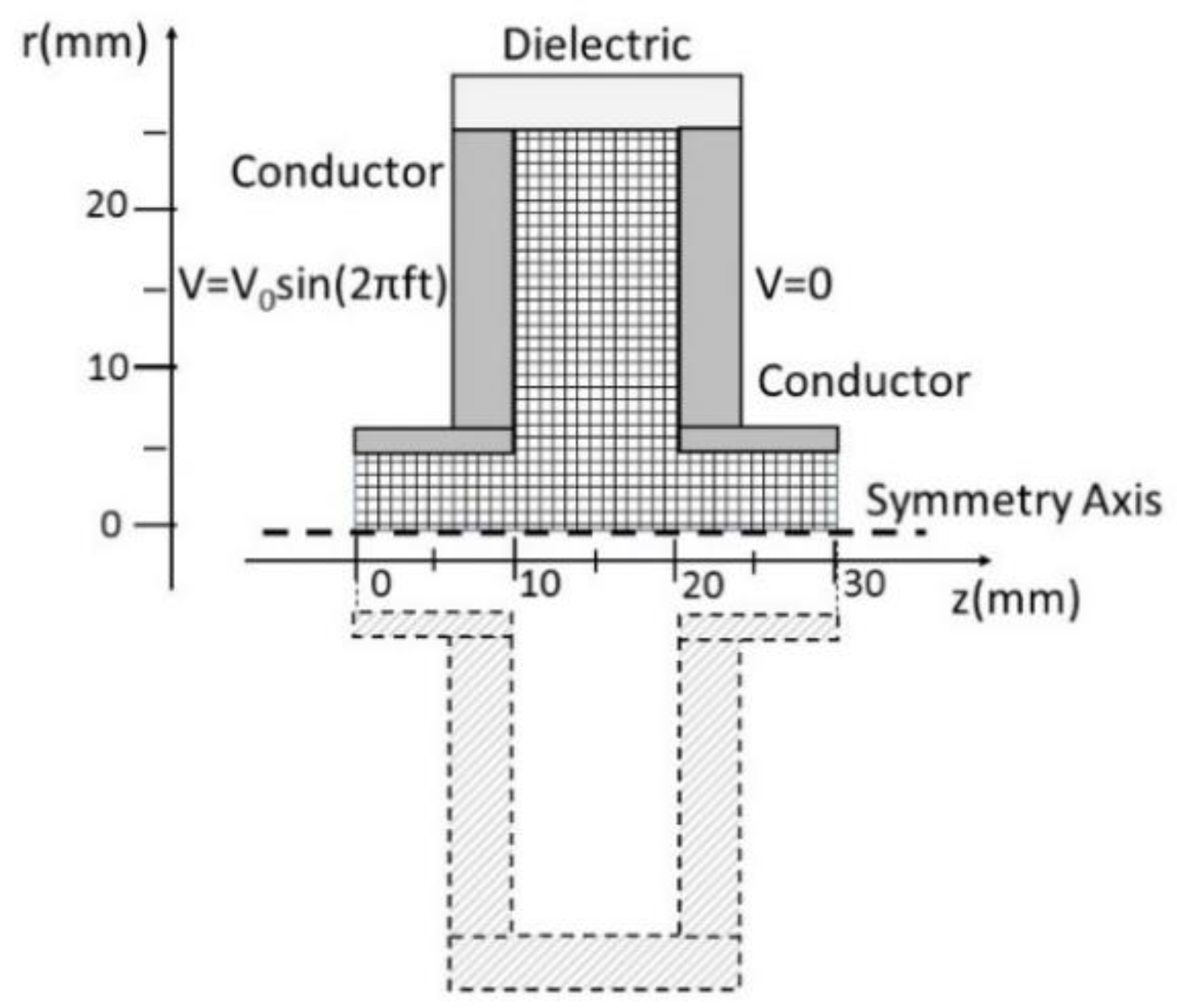
2.2. Two-Dimensional Fluid Model
2.2.1. Model Equations
2.2.2. Boundary Conditions
3. Results and Discussion
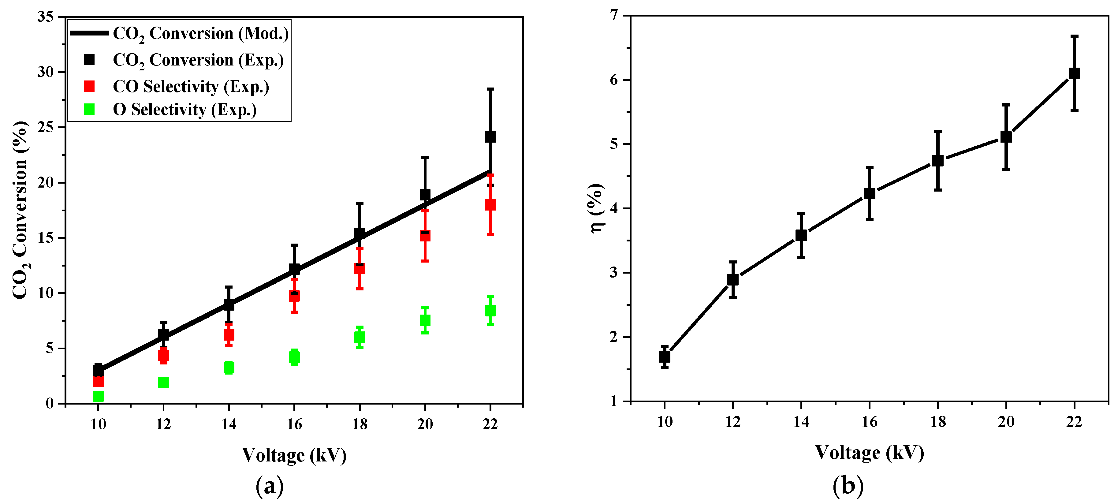
3.1. Experimental Results
3.1.1. Gas Chromatography
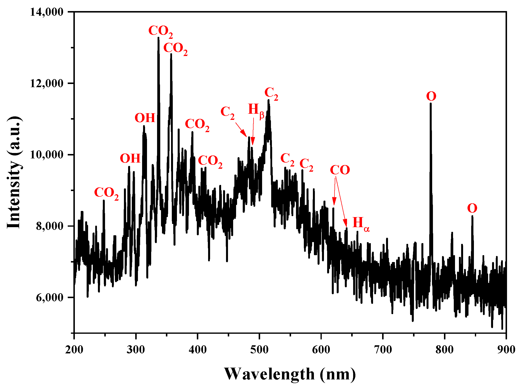
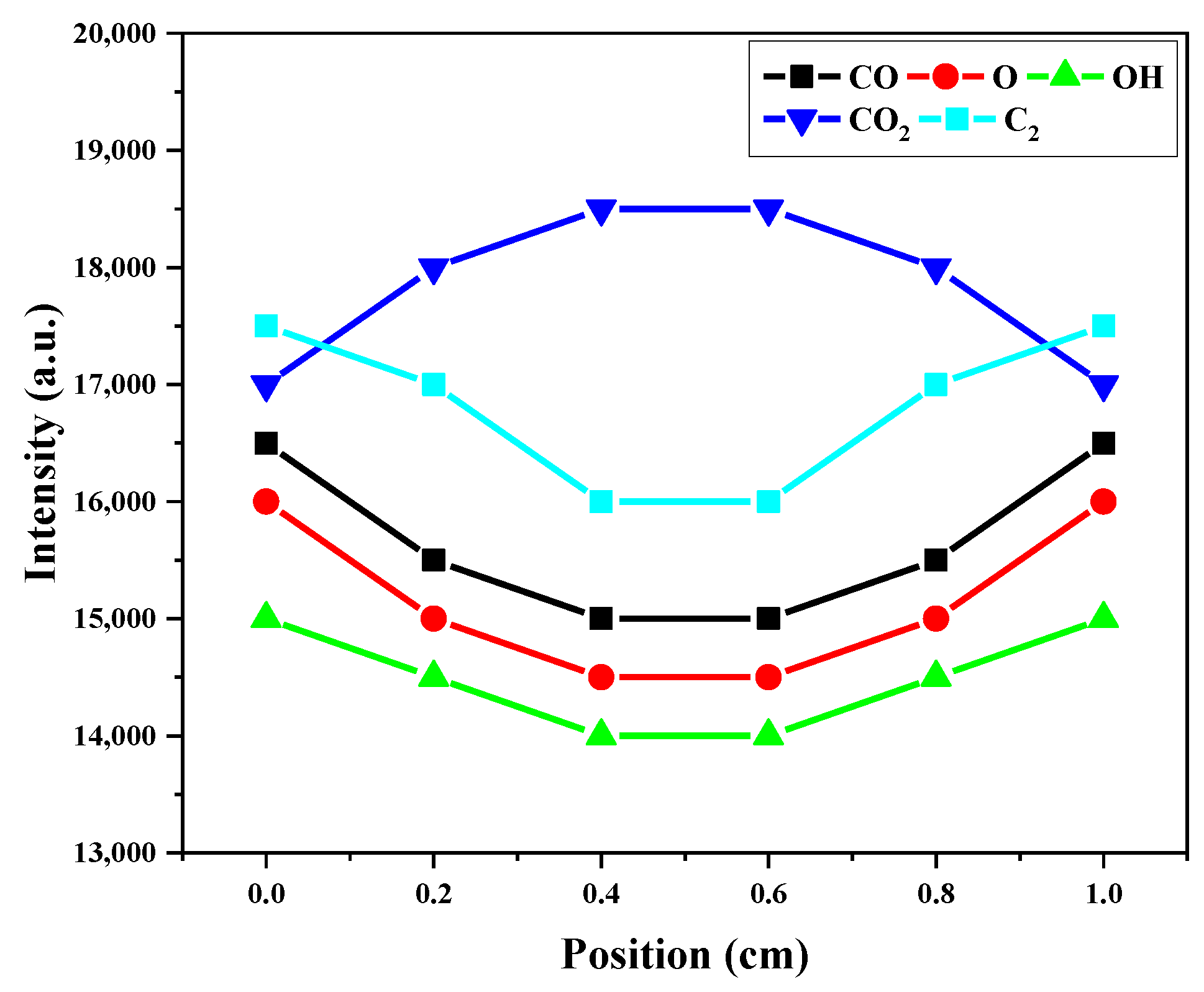
3.1.2. Optical Emission Spectroscopy
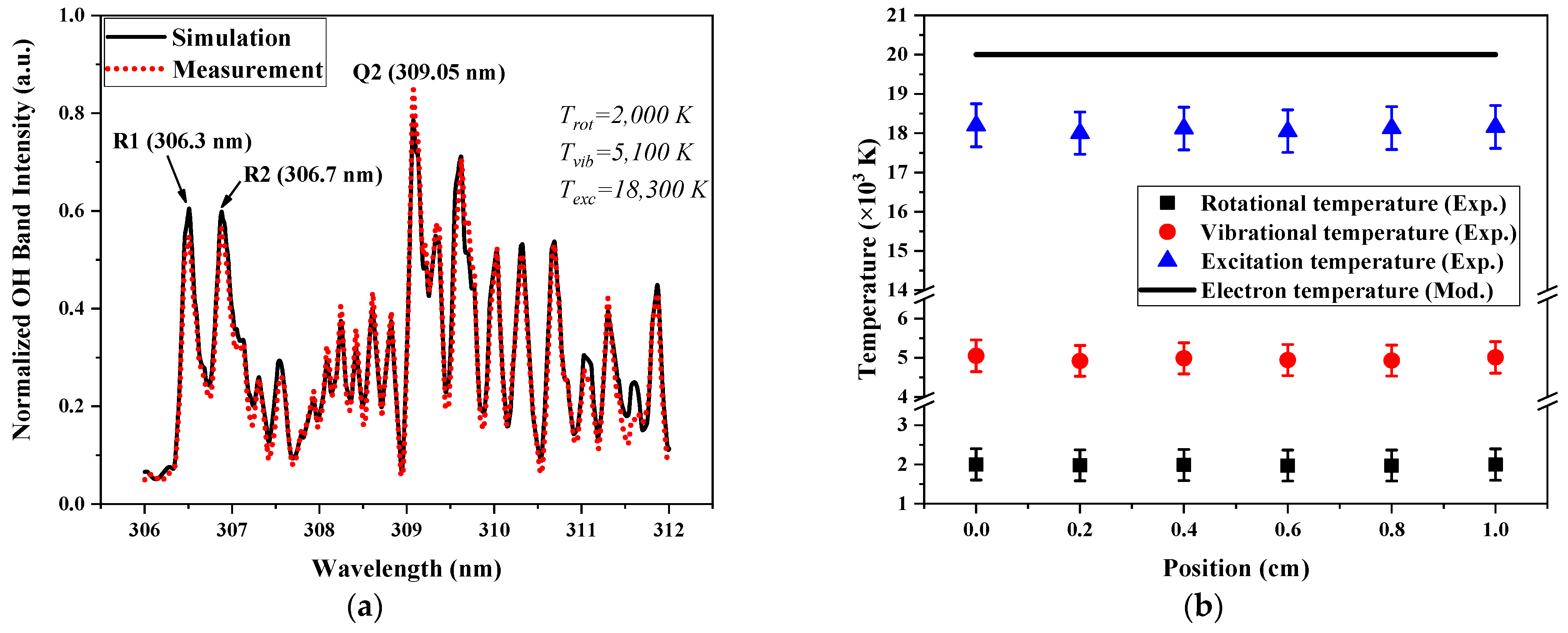
Rotational, Vibrational, and Excitation Temperatures
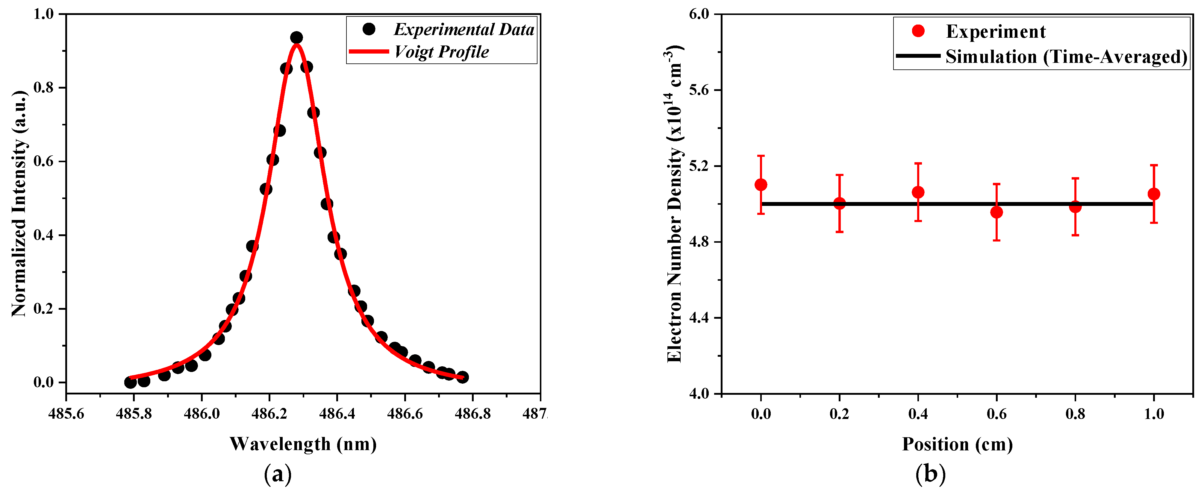
Electron Number Density
3.2. Model Results
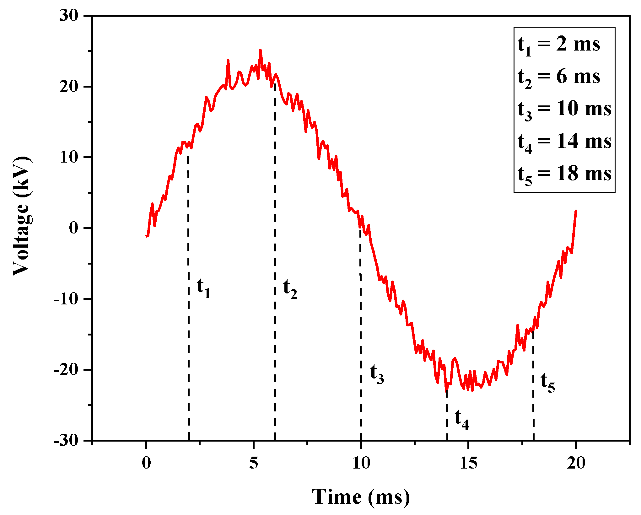
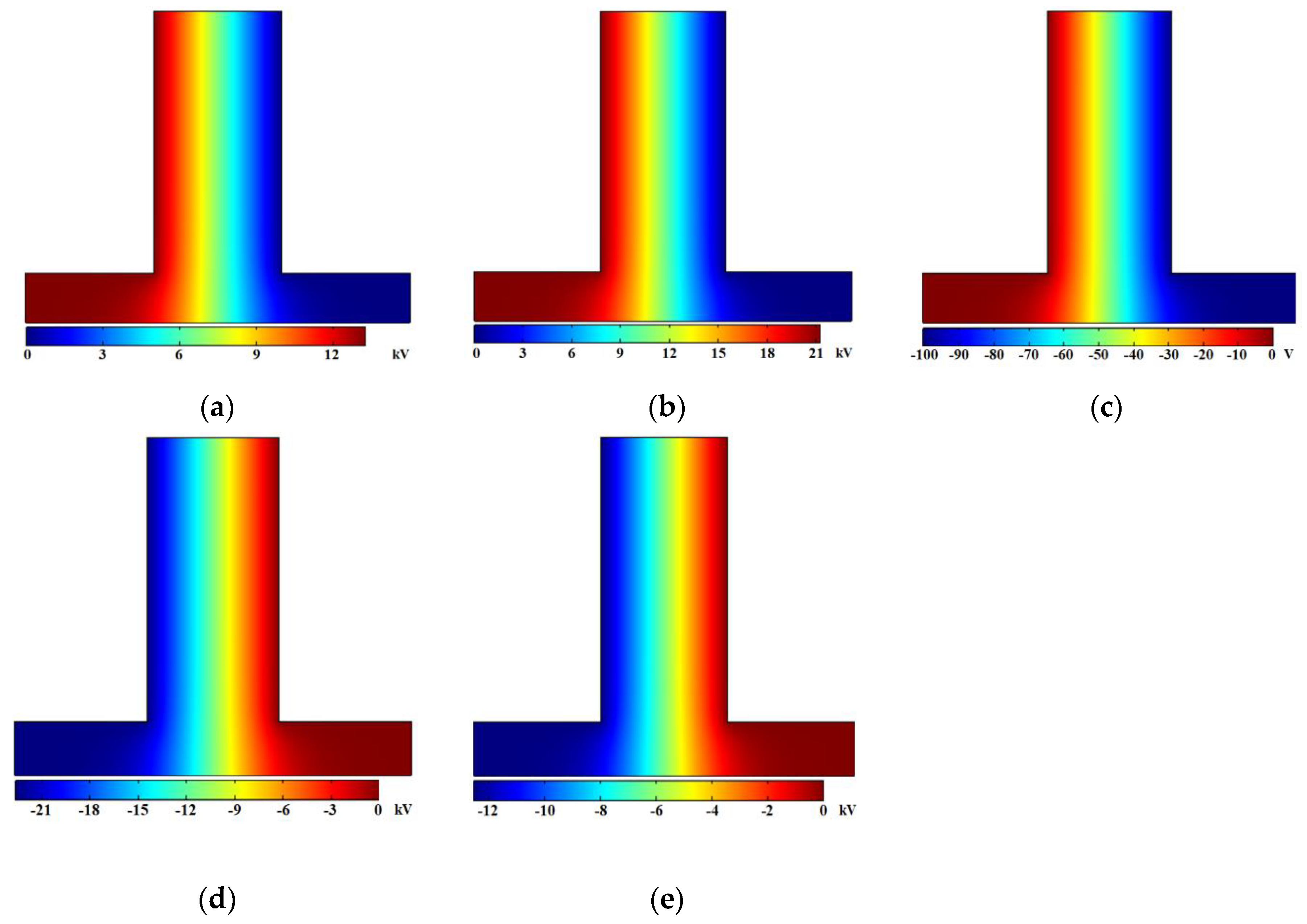
3.2.1. Electric Potential
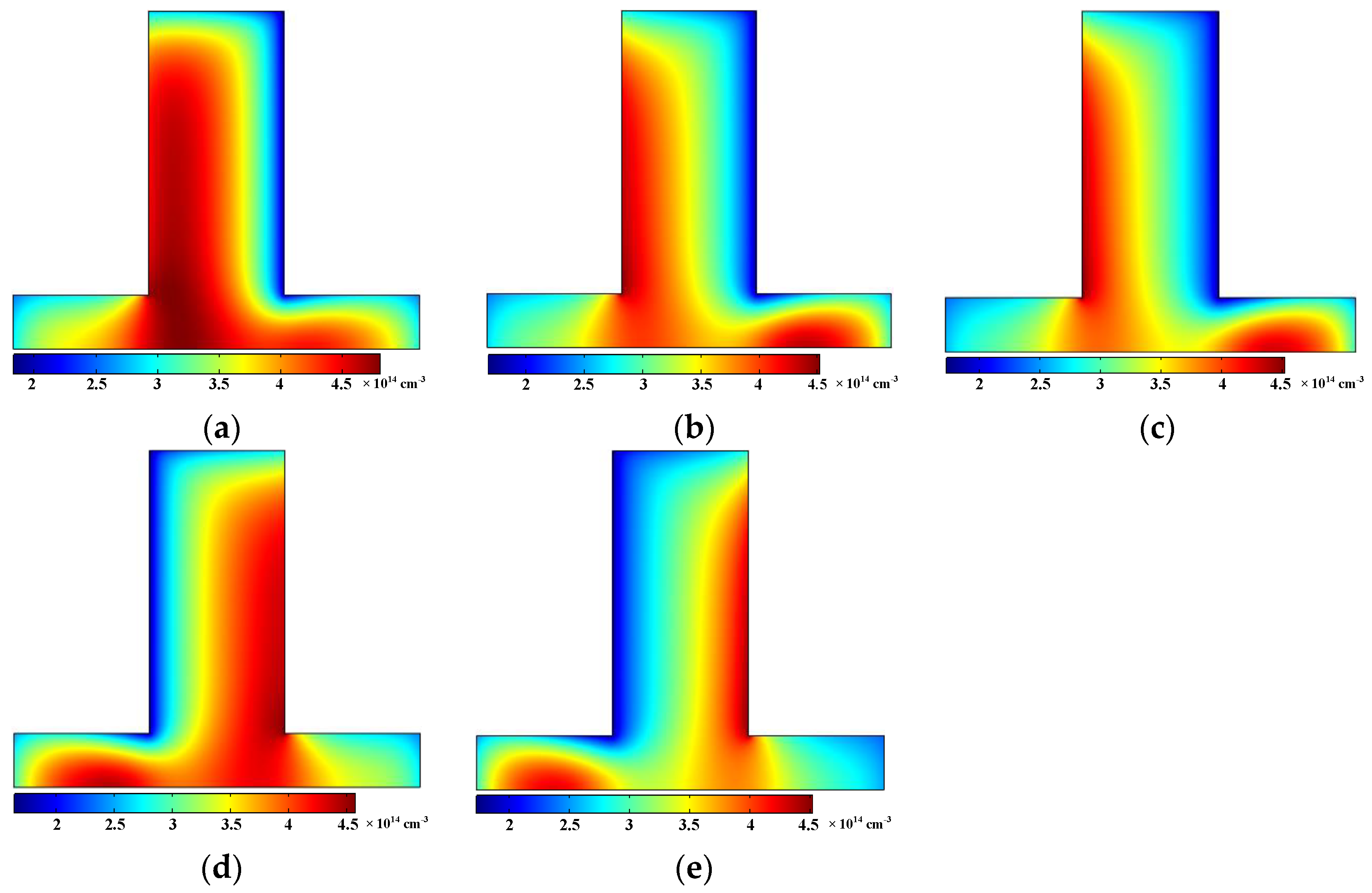
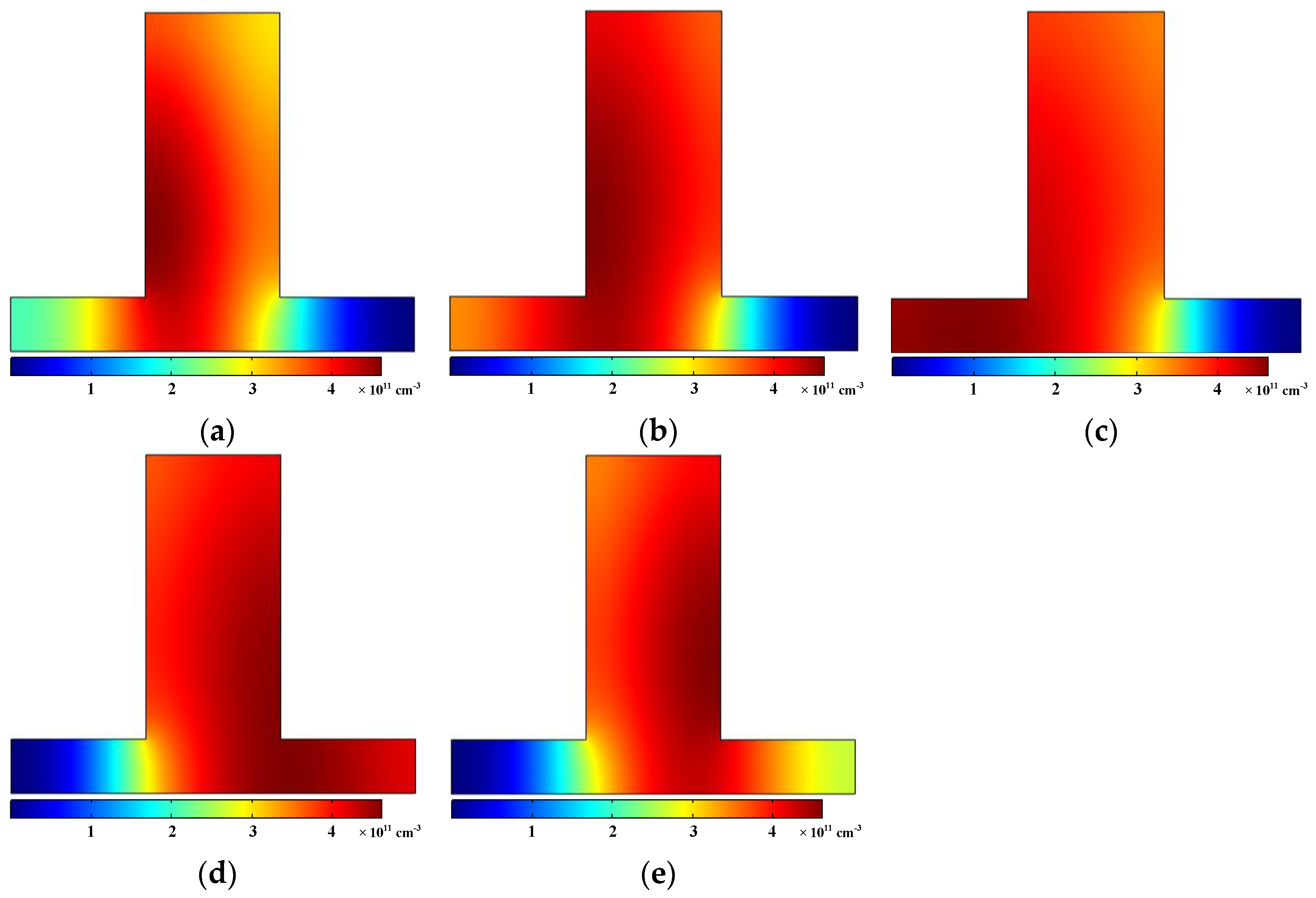
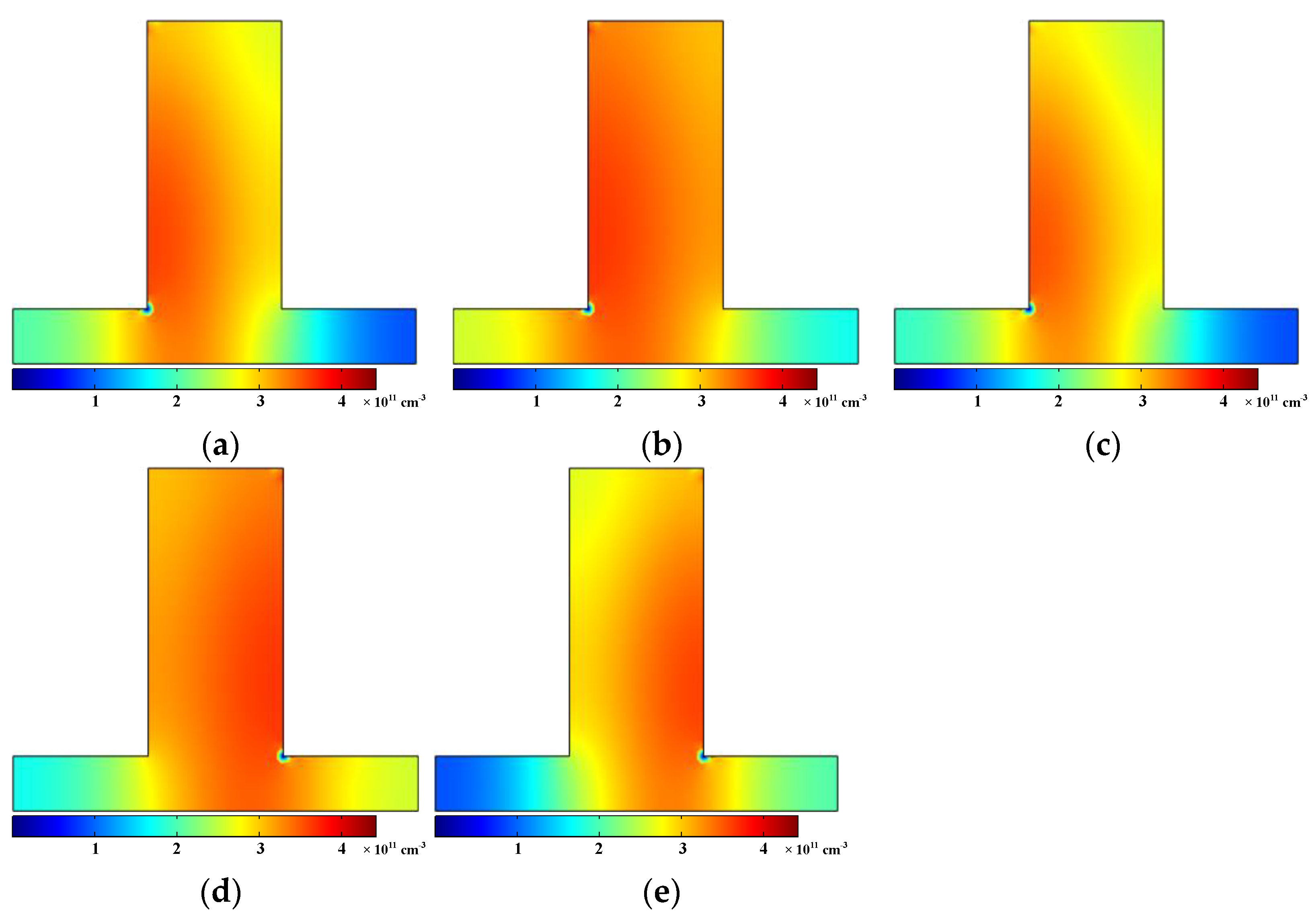
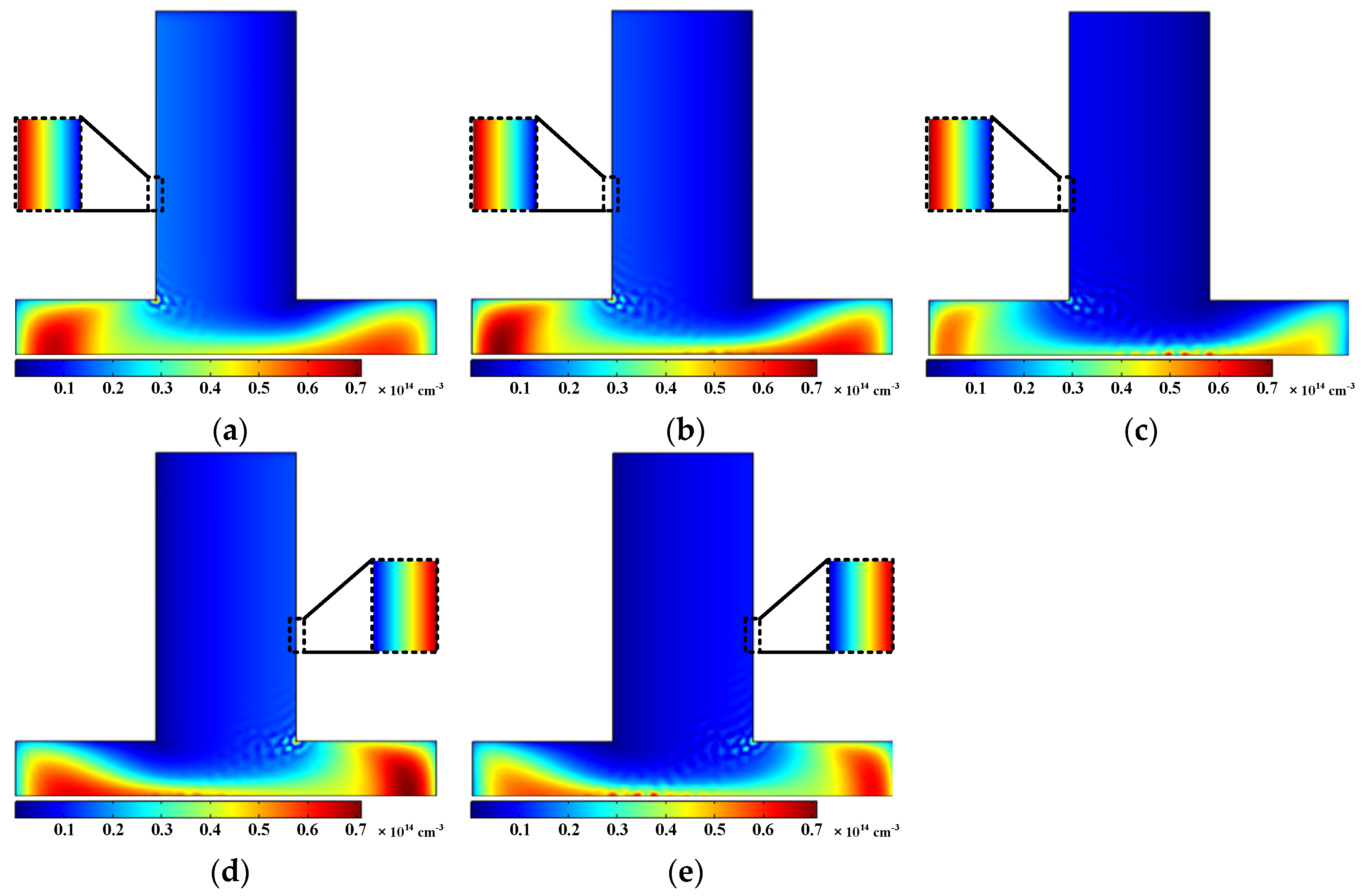
3.2.2. Electron Density
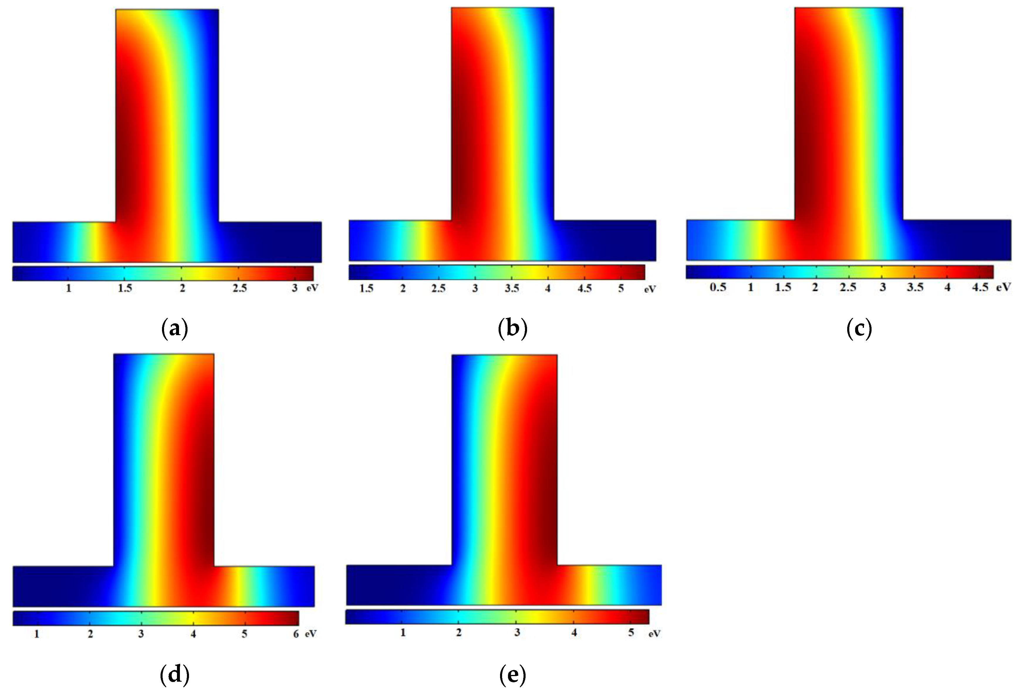
3.2.3. Electron Temperature
3.2.4. CO2 Splitting
- -
- the electron impact dissociation (or dissociative de-excitation collision) producing CO and O (see reactions 7 and 9 in Table 1),
- -
- the electron ionization producing CO2+ ions (see reaction 12 in Table 1),
- -
- the electron dissociative attachment producing CO molecules and O− ions (see reaction 15 in Table 1).
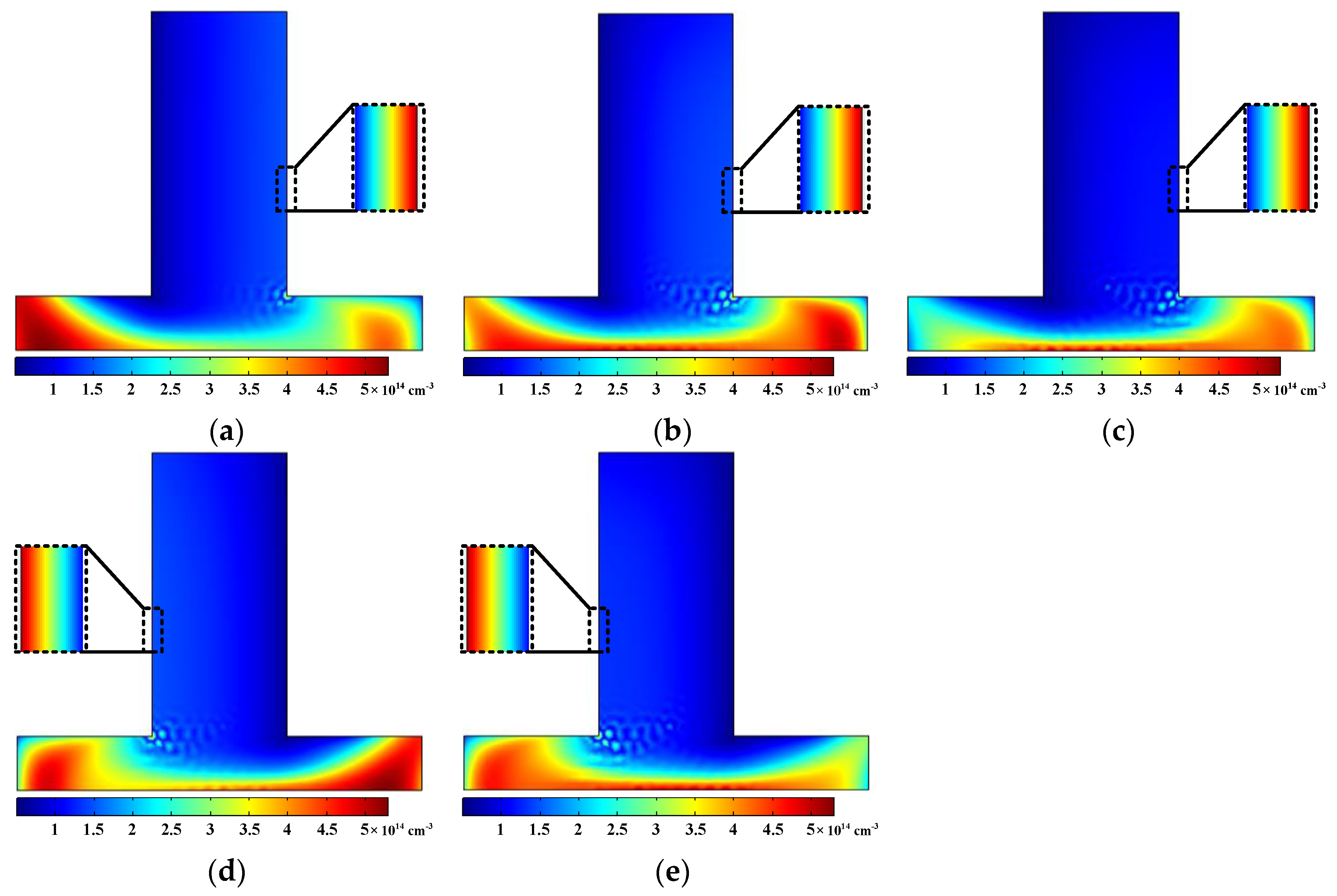
Density of CO2+ Ion
Density of Neutral Species CO, O, and O2
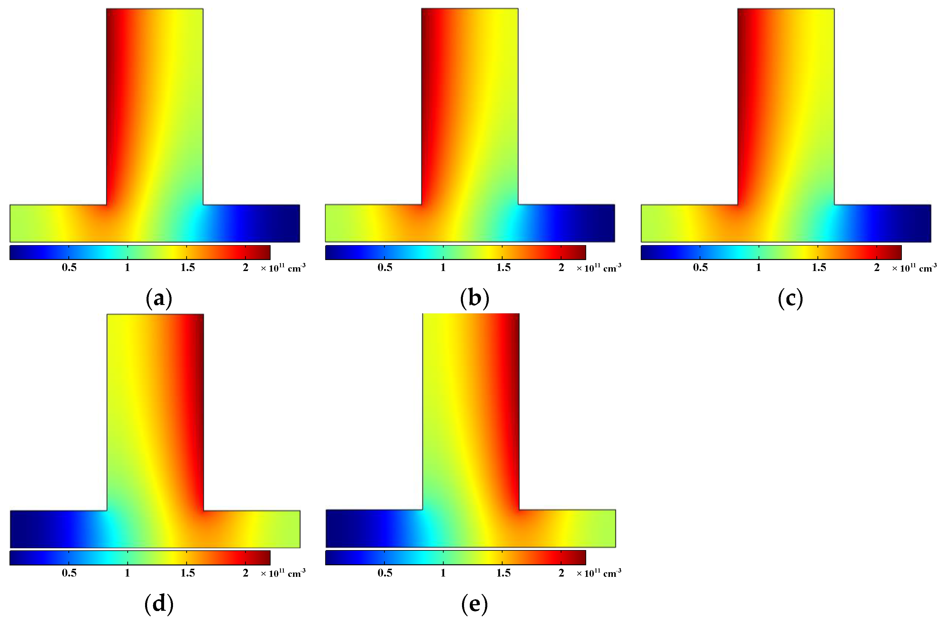
Density of O− Ion
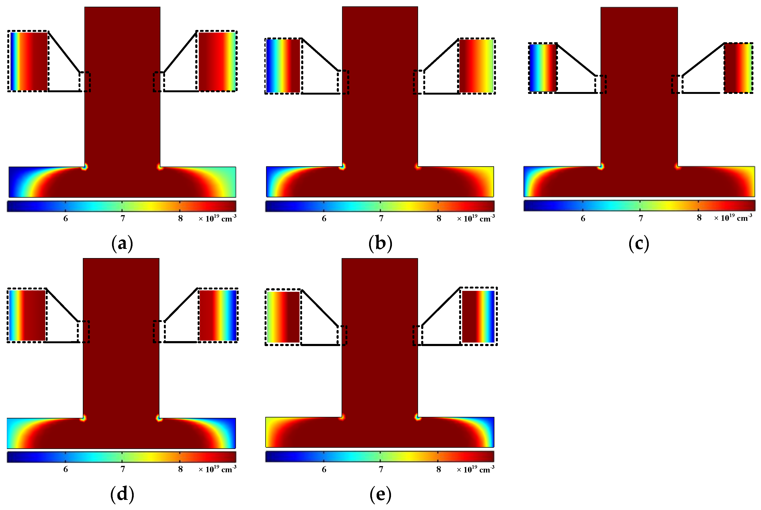
Density of CO2 Molecules
4. Conclusions
Author Contributions
Funding
Institutional Review Board Statement
Informed Consent Statement
Data Availability Statement
Acknowledgments
Conflicts of Interest
References
- Liebermanm, M.A.; Lichtenberg, A.J. Principles of Plasma Discharges and Materials Processing, 2nd ed.; John Wiley & Sons: New York, NY, USA, 2005; pp. 122–250. [Google Scholar]
- Kogelschatz, U. Dielectric-barrier discharges: Their history, discharge physics, and industrial applications. Plasma Chem. Plasma Process. 2003, 23, 1–46. [Google Scholar] [CrossRef]
- Aresta, M. Carbon Dioxide as Chemical Feedstock, 1st ed.; John Wiley & Sons: New York, NY, USA, 2010; pp. 152–180. [Google Scholar]
- Kraus, M.; Eliasson, B.; Kogelschatz, U.; Wokaun, A. CO2 reforming of methane by the combination of dielectric-barrier discharges and catalysis. Phys. Chem. Chem. Phys. 2001, 3, 294–300. [Google Scholar] [CrossRef]
- Fridman, A. Plasma Chemistry, 1st ed.; Cambridge University Press: Cambridge, UK, 2008; pp. 231–254. [Google Scholar]
- Trencheva, G.; Nikiforov, A.; Wanga, W.; Kolevc, S.; Bogaerts, A. Atmospheric pressure glow discharge for CO2 conversion: Model-based exploration of the optimum reactor configuration. Chem. Eng. J. 2019, 362, 830–841. [Google Scholar] [CrossRef]
- Snoeckx, R.; Bogaerts, A. Plasma technology—A novel solution for CO2 conversion? Chem. Soc. Rev. 2017, 46, 5805–5863. [Google Scholar] [CrossRef] [PubMed] [Green Version]
- Li, D.; Li, X.; Bai, M.; Tao, X.; Shang, S.; Dai, X.; Yin, Y. CO2 Reforming of CH4 by Atmospheric Pressure Glow Discharge Plasma: A High Conversion Ability. Int. J. Hydrogen Energy 2009, 34, 308–313. [Google Scholar] [CrossRef]
- Li, H.; Zhou, Y.; Donnelly, V.M. Optical and Mass Spectrometric Measurements of the CH4–CO2 Dry Reforming Process in a Low Pressure, Very High Density, and Purely Inductive Plasma. J. Phys. Chem. A 2020, 124, 7271–7282. [Google Scholar] [CrossRef] [PubMed]
- Li, M.; Xu, G.; Tian, Y.; Chen, L.; Fu, H. Carbon Dioxide Reforming of Methane Using DC Corona Discharge Plasma Reaction. J. Phys. Chem. A 2004, 108, 1687–1693. [Google Scholar] [CrossRef]
- Yu, Q.; Kong, M.; Liu, T.; Fei, J.; Zheng, X. Characteristics of the decomposition of CO2 in a dielectric packed-bed plasma reactor. Plasma Chem. Plasma Process. 2012, 32, 153–163. [Google Scholar] [CrossRef]
- Wang, Q.; Shi, H.; Yan, B.; Jin, Y.; Cheng, Y. Steam enhanced carbon dioxide reforming of methane in DBD plasma reactor. Int. J. Hydrogen Energy 2011, 36, 8301–8306. [Google Scholar] [CrossRef]
- Liu, C.J.; Xu, G.H.; Wang, T. Non-thermal plasma approaches in CO2 utilization. Fuel Process. Technol. 1999, 58, 119–134. [Google Scholar] [CrossRef]
- Shrestha, R.; Tyata, R.; Subedi, D. Estimation of electron temperature in atmospheric pressure dielectric barrier discharge using line intensity ratio method. Kathmandu Univ. J. Sci. Eng. Technol. 2013, 8, 37–42. [Google Scholar] [CrossRef] [Green Version]
- Raju, G.G. Gaseous Electronics Theory and Practice, 1st ed.; CRC Press Taylor & Francis Group: New York, NY, USA, 2006; pp. 351–423. [Google Scholar]
- Torres, J.; Van De Sande, M.J.; Van Der Mullen, J.; Gamero, A.; Sola, A. Stark broadening for simultaneous diagnostics of the electron density and temperature in atmospheric microwave discharges. Spectrochim. Acta B At. Spectrosc. 2006, 61, 58–68. [Google Scholar] [CrossRef]
- Laux, C.O.; Spence, T.G.; Kruger, C.H.; Zare, R.N. Optical diagnostics of atmospheric pressure air plasmas. Plasma Sources Sci. Technol. 2003, 12, 125. [Google Scholar] [CrossRef]
- Dorai, R. Modeling of Plasma Remediation of NOx Using Global Kinetic Models Accounting for Hydrocarbons. Master’s Thesis, University of Illinois at Urbana-Champaign, Champaign, IL, USA, 2000. [Google Scholar]
- Hayashi Database. Available online: www.lxcat.net/Hayashi (accessed on 19 March 2020).
- Wang, W.; Berthelot, A.; Kolev, S.; Tu, X.; Bogaerts, A. CO2 conversion in a gliding arc plasma: 1D cylindrical discharge model. Plasma Sources Sci. Technol. 2016, 25, 065008. [Google Scholar] [CrossRef]
- PLASIMO Software. Plasma Matters. Eindhoven University of Technology. Available online: http://plasimo.phys.tue.nl/ (accessed on 19 March 2020).
- Moravej, M.; Yang, X.; Hicks, R.F.; Penelon, J.; Babayan, S.E. A radio-frequency nonequilibrium atmospheric pressure plasma operating with argon and oxygen. J. Appl. Phys. 2006, 99, 093305. [Google Scholar] [CrossRef]
- Kozák, T.; Bogaerts, A. Splitting of CO2 by vibrational excitation in non-equilibrium plasmas: A reaction kinetics model. Plasma Sources Sci. Technol. 2014, 23, 045004. [Google Scholar] [CrossRef]
- Mikoviny, T.; Kocan, M.; Matejcik, S.; Mason, N.J.; Skalny, J.D. Experimental study of negative corona discharge in pure carbon dioxide and its mixtures with oxygen. J. Phys. Appl. Phys. 2004, 37, 64–73. [Google Scholar] [CrossRef]
- Barkhordari, A.; Mirzaei, S.I.; Falahat, A.; Rodero, A. Numerical and experimental study of an Ar/CO2 plasma in a point-to-plane reactor at atmospheric pressure. Spectrochim. Acta Part B At. Spectrosc. 2021, 177, 106048. [Google Scholar]
- Chiper, A.S.; Chen, W.; Mejlholm, O.; Dalgaard, P.; Stamate, E. Atmospheric pressure plasma produced inside a closed package by a dielectric barrier discharge in Ar/CO2 for bacterial inactivation of biological samples. Plasma Sources Sci. Technol. 2011, 20, 025008. [Google Scholar] [CrossRef]
- Prigogine, I. Chemical kinetics and dynamics. Ann. N. Y. Acad. Sci. 2003, 988, 128–132. [Google Scholar] [CrossRef] [PubMed]
- Marrero, T.; Mason, E.A. Gaseous diffusion coefficients. J. Phys. Chem. Ref. Data 1972, 1, 3–118. [Google Scholar] [CrossRef]
- Jasper, A.W.; Miller, J.A. Lennard–Jones parameters for combustion and chemical kinetics modeling from full-dimensional intermolecular potentials. Combust. Flame 2014, 161, 101–110. [Google Scholar] [CrossRef]
- Raizer, Y.P.; Kisin, V.I.; Allen, J.E. Gas Discharge Physics, 1st ed.; Springer: Berlin/Heidelberg, Germany, 1991; pp. 283–301. [Google Scholar]
- Becker, M.; Loffhagen, D.; Schmidt, W. A stabilized finite element method for modeling of gas discharges. Comput. Phys. Commun. 2009, 180, 1230–1241. [Google Scholar] [CrossRef]
- Hagelaar, G.; De Hoog, F.; Kroesen, G. Boundary conditions in fluid models of gas discharges. Phys. Rev. E 2000, 62, 1452. [Google Scholar] [CrossRef] [PubMed]
- Aerts, R.; Somers, W.; Bogaerts, A. Carbon dioxide splitting in a dielectric barrier discharge plasma: A combined experimental and computational study. ChemSusChem 2015, 8, 702–716. [Google Scholar] [CrossRef] [PubMed]
- Reyes, P.G.; Gomez, A.; Vergara, J.; Martinez, H.; Torres, C. Plasma diagnostics of glow discharges in mixtures of CO2 with noble gases. Rev. Mex. Fis. 2017, 63, 363–371. [Google Scholar]
- Shimizu, K.; Oda, T. Emission spectrometry for discharge plasma diagnosis. Sci. Technol. Adv. Mater. 2001, 2, 577. [Google Scholar] [CrossRef] [Green Version]
- Maouhoub, E. Determination of the real experimental composition of the Ar-CO2 mixture from calculation of the atomic excitation temperature. EPJ Appl. Phys. 1998, 3, 81–89. [Google Scholar] [CrossRef]
- Griem, H.R. Plasma Spectroscopy, 2nd ed.; Cambridge University Press: Cambridge, UK, 2005; pp. 342–390. [Google Scholar]
- Gigosos, M.A.; Cardenoso, V. New plasma diagnosis tables of hydrogen Stark broadening including ion dynamics. J. Physical B-At. Mol. Opt. 1996, 29, 4795. [Google Scholar] [CrossRef]
- Belostotskiy, S.G.; Ouk, T.; Donnelly, V.M.; Economou, D.J.; Sadeghi, N. Gas temperature and electron density profiles in an argon dc microdischarge measured by optical emission spectroscopy. J. Phys. D Appl. Phys. 2010, 107, 053305. [Google Scholar] [CrossRef]
- Nikiforov, A.Y.; Leys, C.; Gonzalez, M.A.; Walsh, J.L. Electron density measurement in atmospheric pressure plasma jets: Stark broadening of hydrogenated and non-hydrogenated lines. Plasma Sources Sci. Technol. 2015, 24, 034001. [Google Scholar] [CrossRef]
- Boffard, J.B.; Lin, C.C.; DeJoseph, C.A., Jr. Application of excitation cross sections to optical plasma diagnostics. J. Phys. D Appl. Phys. 2004, 37, R143. [Google Scholar] [CrossRef]
- Mehr, F.J.; Biondi, M.A. Electron-temperature dependence of electron-ion recombination in Argon. Phys. Rev. 1968, 176, 322. [Google Scholar] [CrossRef]
- Pandhija, S.; Rai, A.K. In situ multielemental monitoring in coral skeleton by CF-LIBS. Appl. Physical B 2009, 94, 545–552. [Google Scholar] [CrossRef]
- Braun, D.; Gibalov, V.; Pietsch, G. Two-dimensional modelling of the dielectric barrier discharge in air. Plasma Sources Sci. Technol. 1992, 1, 166. [Google Scholar] [CrossRef]
- Moreno Wandurraga, S.H. Reduced Reaction Kinetics Model for CO2 Dissociation in Non-Thermal Microwave Discharges. Master’s Thesis, Delft University of Technology, Delft, The Netherlands, 2015. [Google Scholar]
- Khodja, K.; Belasri, A. Sheath formation study in Ne-Xe DBD discharge. Radiat. Eff. Defects Solids 2012, 167, 734–742. [Google Scholar] [CrossRef]
- Staack, D.; Farouk, B.; Gutsol, A.; Fridman, A. Characterization of a dc atmospheric pressure normal glow discharge. Plasma Sources Sci. Technol. 2005, 14, 700. [Google Scholar] [CrossRef]
- Bogaerts, A.; Snoeckx, R.; Trenchev, G.; Wang, W. Plasma Chemistry and Gas Conversion; BoD–Books on Deman: Norderstedt, Germany, 2018. [Google Scholar]


| Num. | Process Name | Reactions | Reaction Rate Constants | Ref. |
|---|---|---|---|---|
| Electron Collisions | ||||
| 1 | Vibrational Excitation | [19] | ||
| 2 | Vibrational Excitation | [19] | ||
| 3 | Vibrational Excitation | [19] | ||
| 4 | Vibrational Excitation | [19] | ||
| 5 | Vibrational Excitation | [19] | ||
| 6 | Electronic Excitation | [21] | ||
| 7 | Dissociative De-excitation Collision | [19] | ||
| 8 | Electron Ionization | [19] | ||
| 9 | Electron Dissociation | [19] | ||
| 10 | Electronic Excitation | [21] | ||
| 11 | Elastic Collision | [21] | ||
| 12 | Electron Ionization | [22] | ||
| 13 | Electron Ionization | [22] | ||
| 14 | Dissociative Electron-Ion Recombination | [22] | ||
| 15 | Dissociative Attachment | [23] | ||
| 16 | Electron Dissociation | [23] | ||
| Atomic Collisions | ||||
| 17 | Neutral Dissociation | [20] | ||
| 18 | Charge Exchange | [20] | ||
| 19 | Scattering | [20] | ||
| 20 | 3-body Recombination | [23] | ||
| 21 | 3-body Neutral-Neutral Collision | [24] | ||
| 22 | 3-body Neutral-Neutral Collision | [24] | ||
| Neutrals | , , ,, |
| Pos. ions | , , , |
| Neg. ions | |
| Elec. excited | |
| Vib. excited | , |
| Applied Voltage (kV) | Power (W) | η (%) |
|---|---|---|
| 10 | 50.95 | 1.69 |
| 12 | 61.60 | 2.89 |
| 14 | 71.35 | 3.58 |
| 16 | 82.14 | 4.23 |
| 18 | 92.64 | 4.74 |
| 20 | 105.49 | 5.11 |
| 22 | 113.05 | 6.1 |
| Technology | Range of CO2 Conversion (%) | Range of Energy Efficiency (%) |
|---|---|---|
| Dielectric Barrier Discharges | 0–30 | 0–15 |
| Microwave Discharges | 0–80 | 0–40 |
| Gliding Arc Discharges | 0–10 | 0–30 |
| AC-PPP Reactor * | 2.5–25 | 1–6 |
| Species | (nm) | Transition Name | Transition Symbol | ||
|---|---|---|---|---|---|
| OH(Q) | 306–312 | Molecular Transition | 0 | 0 | |
| 326.1 | Fox, Duffendack and Barker’s System | 3 | 1a | ||
| 338.3 | Fox, Duffendack and Barker’s System | 2 | 0 | ||
| 368.2 | Fox, Duffendack and Barker’s System | 1 | 2 | ||
| 387.5 | Fox, Duffendack and Barker’s System | 2 | 4 | ||
| 407.3 | Fox, Duffendack and Barker’s System | 1 | 4 | ||
| H | 486.1 | Hβ Balmer series line | n = 4 n = 2 | - | - |
| 656.3 | Hα Balmer series line | n = 3 n = 2 | - | - | |
| 471.6 | Swan System | 0 | 1 | ||
| 516.4 | Swan System | 0 | 0 | ||
| 560.1 | Swan System | 1 | 0 | ||
| 589.5 | High Pressure Bands | 6 | 8 | ||
| 458.5 | The Triplet Bands | 6 | 0 | ||
| 564.2 | The Triplet Bands | 2 | 0 | ||
| 601.4 | The Triplet Bands | 1 | 0 | ||
| 643.2 | The Triplet Bands | 0 | 0 | ||
| 427.3 | Comet-tail system (First Negative System) | 2 | 0 | ||
| 385.3 | Chamberlains Airglow System | 0 | 1 | ||
| 550–600 | Molecular emission Band | 0 | 1 | ||
| O | 777.1 | Atomic Transition | - | - | |
| 843.2 | Atomic Transition | - | - |
| Symbol | Value |
|---|---|
| Mobility, μe, m2/Vs (for electrons) | 1.28 |
| Initial temperatures, T, eV (for electron and heavy particles) | 0.54, 0.026 |
| Potential amplitude, KV | 22 |
| Diffusion coefficient (for electrons) | 0.033 |
| Initial density, cm−3 (charged species) | 1010 |
| Initial density, cm−3 (background species) | 1019 |
| Total time, ms | 20 |
| Time steps, ns | 1 |
Publisher’s Note: MDPI stays neutral with regard to jurisdictional claims in published maps and institutional affiliations. |
© 2021 by the authors. Licensee MDPI, Basel, Switzerland. This article is an open access article distributed under the terms and conditions of the Creative Commons Attribution (CC BY) license (https://creativecommons.org/licenses/by/4.0/).
Share and Cite
Barkhordari, A.; Karimian, S.; Rodero, A.; Krawczyk, D.A.; Mirzaei, S.I.; Falahat, A. Carbon Dioxide Decomposition by a Parallel-Plate Plasma Reactor: Experiments and 2-D Modelling. Appl. Sci. 2021, 11, 10047. https://doi.org/10.3390/app112110047
Barkhordari A, Karimian S, Rodero A, Krawczyk DA, Mirzaei SI, Falahat A. Carbon Dioxide Decomposition by a Parallel-Plate Plasma Reactor: Experiments and 2-D Modelling. Applied Sciences. 2021; 11(21):10047. https://doi.org/10.3390/app112110047
Chicago/Turabian StyleBarkhordari, Ali, Saeed Karimian, Antonio Rodero, Dorota Anna Krawczyk, Seyed Iman Mirzaei, and Amir Falahat. 2021. "Carbon Dioxide Decomposition by a Parallel-Plate Plasma Reactor: Experiments and 2-D Modelling" Applied Sciences 11, no. 21: 10047. https://doi.org/10.3390/app112110047
APA StyleBarkhordari, A., Karimian, S., Rodero, A., Krawczyk, D. A., Mirzaei, S. I., & Falahat, A. (2021). Carbon Dioxide Decomposition by a Parallel-Plate Plasma Reactor: Experiments and 2-D Modelling. Applied Sciences, 11(21), 10047. https://doi.org/10.3390/app112110047