Abstract
The dynamics of the particle size distribution (PSD) of polydispersed fuel spray is important in the evaluation of the combustion process. A better understanding of the dynamics can provide a tool for selecting a PSD that will more effectively meet the needs of the system. In this paper, we present an efficient and elegant method for evaluating the dynamics of the PSD. New insights into the behaviour of polydispersed fuel spray were obtained. A simplified theoretical model was applied to the experimental data and a known approximation of the polydispersed fuel spray. This model can be applied to any distribution, not necessarily an experimental distribution or approximation, and involves a time-dependent function of the PSD. Such simplified models are particularly helpful in qualitatively understanding the effects of various sub-processes. Our main results show that during the self-ignition process, the radii of the droplets decreased as expected, and the number of smaller droplets increased in inverse proportion to the radius. An important novel result (visualised by graphs) demonstrates that the mean radius of the droplets initially increases for a relatively short period of time, which is followed by the expected decrease. Our modified algorithm is superior to the well-known ‘parcel’ approach because it is much more compact; it permits analytical study because the right-hand sides of the mathematical model are smooth, and thus eliminates the need for a numerical algorithm to transition from one parcel to another. Moreover, the method can provide droplet radii resolution dynamics because it can use step functions that accurately describe the evolution of the radii of the droplets. The method explained herein can be applied to any approximation of the PSD, and involves a comparatively negligible computation time.
1. Introduction
A polydispersed fuel spray consists of tens of thousands of droplets with completely different radii scales [1,2,3]. Thus, to accurately trace the change in each droplet over time, a large number of equations need to be solved. The simplest model, which does not imply interactions between droplets, still requires many equations to be solved. For such complicated models, analytical solutions are not available; hence, numerical methods are required. Because solving such a high number of equations with computers cannot be completed in any reasonable time, a ‘parcel’ approach was adopted [4,5,6,7,8,9,10,11]. However, due to computation limits, the number of ‘parcels’ remains low and does not allow a correct description of the polydispersed fuel spray dynamics.
Any study of particle size distribution (PSD) dynamics can help provide insight into combustion processes. Despite the importance of this aspect of spray combustion, there are few theoretical or numerical studies on this subject, which is mainly due to constraints inherent in the situation being studied (e.g., [12,13,14,15,16]). Most of the main mechanisms of such combustion processes remain unknown. However, the methods and dynamics described herein add to our insights.
The commonly used approximations of the initial experimental polydisperse size distributions are the Rosin–Rammler distribution, Nukiyama–Tanasawa distribution, and gamma distribution [17,18]. These approximations provide comparatively accurate representations of experimental data, which allow extrapolation of values beyond the measurement range. These approximations permit comparatively easy calculations of parameters of interest, because they have already been built into computer software (e.g., MATLAB, MATHEMATICA). However, to the best of our knowledge, there is no single mathematical theory that accurately and precisely fits experimental data. Therefore, in the absence of a theoretical basis, the Rosin–Rammler distribution is commonly used and allows us to describe combustion dynamics using raw experimental data.
Most attempts to theoretically describe combustion processes that accompany polydispersed sprays have resulted in complex systems of highly nonlinear partial differential equations [19,20]. The main difficulty is describing the dynamics of individual droplets or groups of droplets that compose the fuels. Semenov pioneered the description of thermal explosion processes for gaseous fuels using simple ordinary differential equations [21]. History has shown that simplified Semenov-type models can often describe the main characteristics of self-ignition in the homogeneous case [22]. However, the models built on Semenov’s work that focus on sprays quickly became very complex when accounting for various droplet radii [23]. The well-known ‘parcel’ method divides droplets into separate sections, but due to computational complexity, this approach fails to estimate a realistic distribution. In the literature, we did not find any study that used more than 5–6 ‘parcels’, and we attributed this to the increased computational complexity with each additional parcel.
In [24], the authors proposed using smooth probability density functions (PDFs) that approximate discrete droplet radii distributions instead of a separate analysis of individual droplets, the ‘parcel’ approximation. In this study, polydispersity is modelled using smooth PDFs that correspond to the initial distribution of the size of the fuel droplets. This approximation of a polydisperse spray is more accurate than the traditional ‘parcel’ approximation, and permits analytical treatment of the corresponding simplified model. We note that any analytical treatment of the ‘parcel’ models is almost impossible because the right-hand sides of the mathematical model are discontinuous. This is the main reason that they are infrequently used.
In [24], the PDF approximations were compared with the ‘parcel’ approximations for 300 ‘parcels’ and found to be more accurate. Details about this comparison can be found in [24].
The corresponding new models are low-dimensional and compact. In the case of ignition processes, such models use a PDF. The density function is a smooth function of only one variable, which is the droplet’s maximal or mean radius. These models allow us to monitor different PDFs.
The main disadvantage of this approach is the rigid shape of PDFs in time (the smooth PDFs correspond to the initial distribution of the size of the fuel droplets). This allowed us to obtain reasonable estimates of thermal explosion limits, but the detailed properties of a spray’s self-ignition are beyond the scope of this method.
In this study, we succeeded in resolving this problem partially. Here, we propose an equation for the evolution of PDFs over time. We begin with the initial PSD and study its dynamics. This modified method was applied to the well-known Rosin–Rammler, Nukiyama–Tanasawa, and gamma distribution approximations of experimental distributions. The main results show that during the self-ignition process, the droplet radii decrease as expected, while the number of smaller droplets increases in inverse proportion to the radius.
Our algorithm presented here is superior to the well-known ‘parcel’ approach, because our model is much more compact, and the right-hand side of the present model is smooth. As a result, we can use combinations of analytical and computational tools. This algorithm can be applied to any approximation of PSD, and the computation time is negligible.
In this study, we mainly consider the evolution of PDFs over time. We demonstrate the main observations using a simplified model. One reason for this simplification is the need to demonstrate the main features without additional complications using more detailed models. We plan to check the main results for more complicated models in the future.
2. Model Description
We first present the constraints on the combustion models. Then, we present models that incorporate PDFs that depend only on the maximal radius.
Several standard assumptions are commonly used for models that describe the thermal explosion of vaporised fuel droplets. Our model is considered adiabatic, because ignition processes occur faster than heat losses by diffusion processes. The pressure variations were assumed to be negligible [21]. In addition, we assume that the diffusion of the gas phase is insignificant compared to that of the liquid phase, and the heat transfer coefficient is determined by the gas features [25]. We further assume that the liquid temperature is identical to the temperature of the saturated liquid because a quasi-steady-state approximation is reasonable for vaporising droplets [26]. Finally, the reaction is modelled in the simplest possible way as a first-order, highly exothermic chemical reaction. This means that the model is represented as a system of nonlinear ordinary differential equations. Here, we present the mathematical model of polydisperse fuel spray, and the discrete model (more details about the assumption of the model can be found in [23]):
The initial conditions are
For the model above, the droplet radius distribution can be approximated by a smooth PDF. The droplet radii sum is replaced by the integral of the corresponding PDF [17,24]. The motivation for this approximation is based on a standard representation of the Riemann integral as a limit of the Riemann sum. This means that this approximation works better for a high number of parcels and can be less accurate for small numbers of parcels. Formally, we can use any smooth function that satisfies the equality.
Here, we use the sub-index 0 for . We use commonly known distributions such as the Rosin–Rammler, Nukiyama–Tanasawa, and gamma distributions as examples.
The corresponding normalised PDF is given by the following equations:
Note that the integration by variable is an approximation that corresponds to the sum of all the radii of the droplets at the initial time. The droplet estimation by the PDF is superior to the ‘parcel’ approach, because the smooth PDF allows us to extrapolate experimental data for radii that do not appear in the standard measurement. In addition, the PDF is not affected by the limitations of the parcel method. The parcel method describes the droplet distribution poorly, because it usually uses a comparatively small number of parcels due to calculation complexity.
Thus, can be viewed as a function of R.
We define the rectangle function:
Here, are unit step functions.
Using the last expressions, we have
Here, is a corresponding smooth PDF function, such as Rosin–Rammler.
Finally, we obtain a nondimensional model in the spirit of Semenov’s theory. We use the following parameters and nondimensional variables:
The function can be recalculated as a function of :
Finally, we obtain:
The following is a new dimensionless system of equations:
where is a function of the maximal dimensionless radius given in (13).
The non-dimensional initial conditions are as follows:
Remark 1.
Equation (2) has another representation that is useful for our study. Using , we can rewrite it as
Its dimensionless form is as follows:
The right-hand sides of (18) and its dimensionless version are not Lipschitz functions and have a singularity point where . Our analysis of the model does not include the values of that are very close to zero. Let us also mention that for very small radii, the model itself is not strictly relevant [27].
3. Results and Discussion
Three PDFs that are widely used for theoretical interpretations of experimentally measured droplet radii distributions are the Rosin–Rammler distribution [28], the Nukiyama–Tanasawa distribution [29], and the well-known gamma distribution. The distribution parameters fit most of the experimental data. The proposed model was applied to arbitrary general experimental data of a polydispersed fuel spray produced by a plain-jet air-blast atomizer [18] and its approximations. All calculations were performed numerically using MATLAB software. The experimental distribution and its approximations based on known theoretical distributions that are used and normalised are presented in Figure 1.
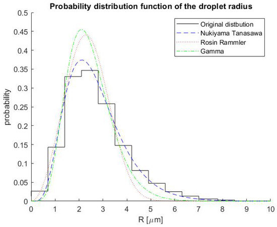
Figure 1.
Normalized experimental probability distributions and various approximations by probability density functions (Nukiyama–Tanasawa, Rosin—Rammler, and gamma distributions) of the droplets’ radii.
In the region close to , we observed an almost linear behaviour of the maximal radius as a function of time. This corresponds to initial fast motion (evaporation). Close to this almost “linear” region, our model is valid; thus, we can study the various types of dynamics that describe the PSD. The integrand of F represents the PSD. This conclusion immediately follows from the definition of F (10). On the other side, the integrand of is proportional to the PSD (it can be seen by Equation (13)). The dynamics of the PSD are based on the initial PSD (initial measurement) and its different approximations by various commonly used PDFs.
As shown in Figure 2, the behaviour of different integrands of is quantitatively very similar. The experimental PSD is discontinuous, because it is discrete and divided into several parcels, whereas all approximations are smooth. The integrands of F consist of , which can be described with the help of PDFs (more accurately, it is proportional to the PDFs).
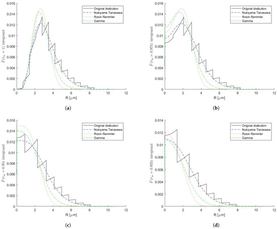
Figure 2.
The integrand of given by Equation (13) in the region near for experimental data and its approximations (Nukiyama–Tanasawa, Rosin–Rammler, and gamma distributions), at various values of . (a) The integrand of at rm = 1. (b) The integrand of at rm = 0.975. (c) The integrand of at rm = 0.95. (d) The integrand of at rm = 0.925.
Recall that the function F is an integral that depends on . In Figure 3, we can see graphs of the integrand of F, and the area under the graph is a visualisation of F. The area can also be interpreted as a function of the droplet mean radius. As the maximum radius decreases, it is reasonable to suppose that the mean radius will decrease as well.
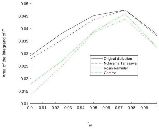
Figure 3.
Integrand of F given by Equation (10).
With the help of the current more accurate model (compared with its previous version [24]), we can observe the dynamical behaviour of the probability functions. The results are shown in Figure 4.
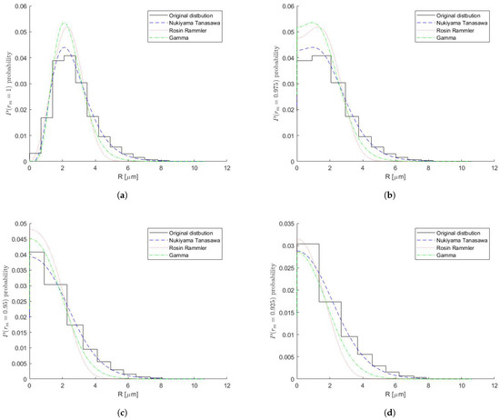
Figure 4.
Nukiyama–Tanasawa, Rosin–Rammler, and gamma probability for various values. (a) Probability at rm = 1. (b) Probability at rm = 0.975. (c) Probability at rm = 0.95. (d) Probability at rm = 0.925.
Our computations demonstrate a different type of behaviour for the mean radius in the initial time period. We observe an increase in the mean radius for a short period of time, followed by the expected behaviour (i.e., the decrease in the mean radius). A similar behaviour was also observed for a different probability function (Figure 5). This phenomenon is stable numerically. We have a heuristic explanation only, and hopefully, one will be derived analytically in the future.
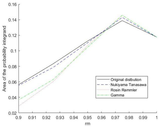
Figure 5.
The area of the probability integrand as a function of the for the various distributions (Nukiyama–Tanasawa, Rosin—Rammler, and gamma).
We can observe this numerical phenomenon of mean radius increase for any studied PDF. For example, let us observe the behaviour of the integrand of the Nukiyama–Tanasawa approximation (Figure 6) in time. For a heuristic explanation of this observation, we can analyse Equation (18) in more detail. Recall Equations (18):
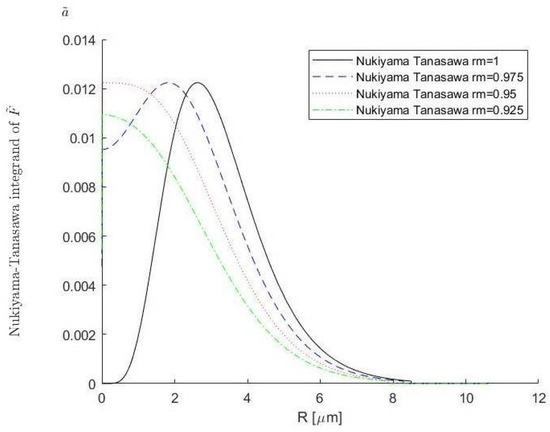
Figure 6.
Nukiyama–Tanasawa integrand of given by Equation (13) for various values of .
For , the gas temperature was higher than the temperature of the droplets, and the derivative was negative. The reduction of droplet radii over time is also valid because the radius decreases in a high-temperature environment. As can be seen, the curve of any droplet density function is shifted to the right with respect to time, as expected. The shift occurs due to the reduction in the droplet size. A more important observation is as follows: For any droplet, the radius reduction is proportional to the inverse of the radius. The last insight indicates that droplets with a large radius will decrease in size more slowly than droplets with a smaller radius. This phenomenon is seen in the graph, where the number of small-radius droplets increases with time.
Consider the following possible explanation: Droplets with a higher ratio between the surface and volume were more influenced by heat. From this remark, it follows that the reduction in the size of smaller droplets is faster than that of larger ones. This can be seen analytically because the derivatives of the radii of the droplets are proportional to the inverse of their radii. Heuristically, this means that smaller droplets have lesser influence on the mean radius than larger ones. Of course, this heuristic explanation is not an accurate explanation, but for the moment, we have no accurate proof of the phenomena.
4. Conclusions
In this study, we modified the approach proposed in our previous work [24], where we used smooth PDFs to approximate droplet radii distributions. This modification helps us follow the dynamics of the PSD. In addition, we studied the time evolution of the PDFs. The low computation time of the proposed approach allowed us to accurately follow the dynamics of the experimentally measured PSD and its different smooth approximations. These smooth approximations allowed us to explore the behaviour of PSDs using a combination of analytical and computational methods. The new tools provided by our model allow infinite accuracy, and can be applied on any theoretical PSD.
An important novel result (which is visualised by graphs) demonstrates that the mean radius of the droplets first increases for a short time, followed by the expected decrease. This means that the maximum mean radius is not located at the beginning of the process, as expected.
Our approach is superior to the well-known ‘parcel’ approach because it does not have the computational problems that limited the ‘parcel’ approach to a small number of parcels. Moreover, the model is much more compact, and the right-hand side of the equations is smooth. Our results show that the mean radius of the droplets eventually decreases, but, surprisingly, initially increases. We associate this phenomenon of the increase in the mean radius to the tendency of smaller droplets to evaporate at a higher rate. The ability to research the evolution of a complex system of droplets in the ignition process opens a window to an interesting new field in the analytical and numerical study of spray combustion.
This new method can be applied to any PSD approximation, and the computation time is negligible. For example, in this study, we applied the new tools to the well-known Rosin–Rammler, Nukiyama–Tanasawa, and gamma distribution approximations of experimental distributions. Our results were in good agreement with the experimental results.
We plan to check the main results for more complicated models in the future.
Author Contributions
S.H.: Numerical simulations. O.N.: Mathematical model. V.G.: Data analysis. All authors have read and agreed to the published version of the manuscript.
Funding
This work was fund by Jerusalem college of technology and Ben Guion University.
Institutional Review Board Statement
Not applicable.
Informed Consent Statement
Not applicable.
Data Availability Statement
We used data available in our paper on combustion.
Conflicts of Interest
No conflict of Interest.
Nomenclature
| A | constant pre-exponential rate factor |
| C | molar concentration (k mol m−3) |
| c | specific heat capacity (J kg−1 K−1) |
| E | activation energy (J k mol−1) |
| L | liquid evaporation energy (i.e., latent heat of evaporation, enthalpy of evaporation) (J kg−1) |
| number of droplets of size i per unit volume (m−3) | |
| Q | combustion energy (J kg−1) |
| B | universal gas constant (J k mol−1 K−1) |
| radius of size i drops (m) | |
| maximal droplet radius at (m) | |
| T | temperature (K) |
| t | time (s) |
| (s) | |
| probability density function | |
| probability distribution function | |
| unit step function | |
| rectangle function | |
| Greek symbols and dimensionless parameters | |
| dimensionless volumetric phase content, | |
| quantity equivalent to the volumetric phase content for the continuous model | |
| dimensionless reduced initial temperature (with respect to the activation temperature ) | |
| dimensionless parameter that represents the reciprocal of the final dimensionless adiabatic temperature of the thermally insulated system after the explosion has been completed | |
| dimensionless parameters introduced in Equation (11) that describe the interaction between gaseous and liquid phases | |
| molar mass (kg kmol−1) | |
| thermal conductivity (W m−1 K−1) | |
| density (kg m−3) | |
| dimensionless time | |
| represents the internal characteristics of the fuel (the ratio of the specific combustion energy to the latent heat of evaporation) and is defined in Equation (11) (dimensionless) | |
| Dimensionless variables | |
| dimensionless fuel concentration | |
| dimensionless temperature | |
| r | dimensionless radius |
| Subscripts | |
| d | liquid fuel droplets |
| f | combustible gas component of the mixture |
| g | gas mixture |
| i | number of droplet sizes |
| L | liquid phase |
| p | under constant pressure |
| s | saturation line (surface of droplets) |
| 0 | initial state |
| m | number of droplet sizes |
| Abbreviations | |
| probability density function | |
| PSD | particle size distribution |
References
- Wirtz, J.; Cuenot, B.; Riber, E. Numerical study of a polydisperse spray counterflow diffusion flame. Proc. Combust. Inst. 2021, 38, 3175–3182. [Google Scholar] [CrossRef]
- Wang, Q.; Jaravel, T.; Ihme, M. Assessment of spray combustion models in large-eddy simulations of a polydispersed acetone spray flame. Proc. Combust. Inst. 2019, 37, 3335–3344. [Google Scholar] [CrossRef]
- Greenberg, J.B.; Katoshevski, D. Polydisperse spray diffusion flames in oscillating flow. Combust. Theory Model. 2016, 20, 349–372. [Google Scholar] [CrossRef]
- Greenberg, J.; Silverman, I.; Tambour, Y. On the origins of spray sectional conservation equations. Combust. Flame 1993, 93, 90–96. [Google Scholar] [CrossRef]
- Tambour, Y. Transient mass and heat transfer from a cloud of vaporizing droplets of various size distributions: A sectional approach. Chem. Eng. Commun. 1986, 44, 183–196. [Google Scholar] [CrossRef]
- Tambour, Y. Simulation of coalescence and vaporization of kerosene fuel sprays in a turbulent jet—A sectional approach. In Proceedings of the 21st Joint Propulsion Conference, Monterey, CA, USA, 8–10 July 1985; American Institute of Aeronautics and Astronautics: Reston, VA, USA, 1985. [Google Scholar]
- Tambour, Y. Vaporization of polydisperse fuel sprays in a laminar boundary layer flow: A sectional approach. Combust. Flame 1984, 58, 103–114. [Google Scholar] [CrossRef]
- Anidjar, F.; Tambour, Y.; Greenberg, J. Mass exchange between droplets during head-on collisions of multisize sprays. Int. J. Heat Mass Transf. 1995, 38, 3369–3383. [Google Scholar] [CrossRef]
- Silverman, I.; Greenberg, J.; Tambour, Y. Stoichiometry and polydisperse effects in premixed spray flames. Combust. Flame 1993, 93, 97–118. [Google Scholar] [CrossRef]
- Tambour, Y.; Zehavi, S. Derivation of near-field sectional equations for the dynamics of polydisperse spray flows: An analysis of the relaxation zone behind a normal shock wave. Combust. Flame 1993, 95, 383–409. [Google Scholar] [CrossRef]
- Silverman, I.; Greenberg, J.B.; Tambour, Y. Asymptotic analysis of a premixed polydisperse spray flame. SIAM J. Appl. Math. 1991, 51, 1284–1303. [Google Scholar] [CrossRef]
- Aggrawal, S.K. A review of spray ignition phenomena: Present status and future research. Prog. Energy Combust. Sci. 1998, 24, 565–600. [Google Scholar] [CrossRef]
- Stone, R. Introduction to Internal Combustion Engines; Macmillan: London, UK, 1998. [Google Scholar]
- Sazhin, E.M.; Sazhin, S.S.; Heikal, M.R.; Babushok, V.I.; Johns, R.A. A detailed modeling of the spray ignition process in diesel engines. Combust. Sci. Technol. 2000, 160, 317–344. [Google Scholar] [CrossRef]
- Greenberg, J.B. Droplet size distribution effects in an edge flame with a fuel spray. Combust. Flame 2017, 179, 228–237. [Google Scholar] [CrossRef]
- Noh, D.; Gallot-Lavallée, S.; Jones, W.P.; Navarro-Martinez, S. Comparison of droplet evaporation models for a turbulent, non-swirling jet flame with a polydisperse droplet distribution. Combust. Flame 2018, 194, 135–151. [Google Scholar] [CrossRef] [Green Version]
- Babinsky, E.; Sojka, P.E. Modeling drop size distributions. Prog. Energy Combust. Sci. 2002, 28, 303–329. [Google Scholar] [CrossRef]
- Urbán, A.; Józsa, V. Investigation of Fuel Atomization with Density Functions. Period. Polytech. Mech. Eng. 2018, 62, 33–41. [Google Scholar] [CrossRef] [Green Version]
- Warnatz, J.; Maas, U.; Dibble, W.R. Combustion: Physical and Chemical Fundamentals, Modeling and Simulation, Experiments, Pollutant Formation; Springer: Berlin/Heidelberg, Germany; New York, NY, USA, 2006. [Google Scholar]
- Kolakaluria, S.S.R.; Panchagnulab, M.V. Trends in multiphase modeling andsimulation of sprays. Int. J. Spray Combust. Dyn. 2014, 6, 317–356. [Google Scholar] [CrossRef]
- Semenov, N.N. Zur theorie des verbrennugsprozesse. Z. Phys. 1928, 48, 571–581. [Google Scholar] [CrossRef]
- Kats, G.; Greenberg, J. Forced thermal ignition of a polydisperse fuel spray. Combust. Sci. Technol. 2018, 190, 849–877. [Google Scholar] [CrossRef]
- Bykov, V.; Goldfarb, I.; Greenberg, V. Auto-ignition of a polydisperse fuel spray. Proc. Combust. Inst. 2007, 31, 2257–2264. [Google Scholar] [CrossRef]
- Nave, O.; Gol’dshtein, V.M.; Bykov, V. A probabilistic model of thermal explosion in polydisperse fuel spray. Appl. Math. Comput. 2010, 217, 2698–2709. [Google Scholar] [CrossRef]
- Sazhin, S.; Martynov, S.; Kristyadi, T.; Crua, C.; Heikal, M.R. Diesel fuel spray penetration, heating, evaporation and ignition: Modelling vs. experimentation. Int. J. Eng. Syst. Model. Simul. 2008, 1, 1–19. [Google Scholar]
- Williams, F.A. The Fundamental Theory of Chemically Reacting Flow System; Benjamin-Cummings: Menlo Park, CA, USA, 1985. [Google Scholar]
- Tyurenkova, V.V. Non-equilibrium diffusion combustion of a fuel droplet. Acta Astronaut. 2012, 75, 78–84. [Google Scholar] [CrossRef]
- Rosin, P.; Rammler, E. Laws governing the fineness of powdered coal. J. Inst. Fuel 1933, 7, 29–36. [Google Scholar]
- Nukiyama, S.; Tanasawa, Y. Experiments on the atomization of liquids in an airstream. Trans. Jpn. Soc. Mech. Eng. 1939, 5, 68–75. [Google Scholar]
Publisher’s Note: MDPI stays neutral with regard to jurisdictional claims in published maps and institutional affiliations. |
© 2021 by the authors. Licensee MDPI, Basel, Switzerland. This article is an open access article distributed under the terms and conditions of the Creative Commons Attribution (CC BY) license (https://creativecommons.org/licenses/by/4.0/).