Collision Avoidance Controller for Unmanned Surface Vehicle Based on Improved Cuckoo Search Algorithm

Abstract

For the dynamic collision avoidance problem of an unmanned surface vehicle (USV), a dynamic collision avoidance control method based on an improved cuckoo search algorithm is proposed. The collision avoidance model for a USV and obstacles is established on the basis of the principle of the velocity obstacle method. Simultaneously, the Convention on the International Regulations for Preventing Collisions at Sea (COLREGS) is incorporated in the collision avoidance process. For the improvement of the cuckoo algorithm, the adaptive variable step-size factor is designed to realize the adaptive adjustment of flight step-size, and a mutation and crossover strategy is introduced to enhance the population diversity and improve the global optimization ability. The improved cuckoo search algorithm is applied to the collision avoidance model to obtain an optimal collision avoidance strategy. According to the collision avoidance strategy, the desired evasion trajectory is obtained, and the tracking controller based on PID is used for the Lanxin USV. The experimental results show the feasibility and effectiveness of the proposed collision avoidance method, which provides a solution for the autonomous dynamic collision avoidance of USVs.

1. Introduction

An unmanned surface vehicle (USV) is an autonomous surface vehicle capable of conducting port patrols and performing special maritime tasks, and has been intensively researched by various countries in recent years [1,2]. A USV is required to perform autonomous avoidance of obstacles on the sea during its maritime tasks, so autonomous collision avoidance control technology has been one of the key technologies for USV research [3].

Recently, some researchers have performed more research on the technology of USV collision avoidance. A motion collision avoidance algorithm for a USV in a dynamic and complex environment has been proposed, which is realized based on the velocity obstacle method and combined with the rules of collision avoidance at sea, so as to complete the autonomous collision avoidance of the USV [4]. In [5], the angular velocity and linear velocity of a USV in the collision avoidance process are calculated, and the angular velocity buffer model is introduced, so as to ensure stable output and realize the avoidance of local static obstacles. A layered collision avoidance method is designed in [6]. The velocity obstacle method and the improved artificial potential field method are used to solve the collision avoidance problem for a USV under normal and emergency conditions, respectively. Xiong et al. [7] present elite group-based evolutionary algorithms based on the simulated annealing algorithm and particle swarm optimization for path planning using multiple USVs. Sun et al. [8] use the fast marching method combined with a model predictive control algorithm to design an autonomous navigation control system. Ref. [9] proposes a fast collision avoidance method based on velocity resolution to realize a fast response for a USV in an unknown complex marine environment. For the path navigation method of a USV, a chaotic and sharing-learning particle swarm optimization algorithm is developed to solve the extended traveling salesman problem and the nonlinear multi-objective model in [10]. These collision avoidance algorithms for USVs include the velocity obstacle method [11], field theory [12,13,14,15], the finite state machine [16], A star [17,18], the LROABRA (local reactive obstacle avoidance based on region analysis) method [15], the VFH+ method [15], the fast marching method [19], and so on. Most of the above literature focuses on the generation of a collision avoidance strategy, but there is not much research on the combination of a collision avoidance strategy and a controller.

In the research for USV collision avoidance strategies, the optimization algorithm is often used to obtain the optimal collision avoidance strategy [20,21]. Song et al. introduced a two-level collision avoidance algorithm and improved the calculation efficiency and accuracy through the particle swarm optimization (PSO) algorithm [6]. For this solution space of the collision avoidance strategy, the objective function is solved by the PSO algorithm in [22]. Guo et al. designed an extended chaos and shared learning PSO (CSPSO) algorithm to solve the traveling salesman problem (TSP) and nonlinear multi-objective model in a collision avoidance algorithm [10]. Xia et al. proposed a modified quantum PSO (MQPSO) method to obtain the optimal velocity variation of a USV to avoid collision and reduce energy consumption [23]. Lazarowska proposed a path-planning method in a dynamic environment based on ant colony optimization (ACO) [24]. Subsequently, the method was applied in a ship control system [25]. Wang et al. proposed an improved ACO algorithm to solve the problem of insufficient search ability in a collision avoidance planning algorithm for a USV [26]. The improved pseudo-random proportion rule was used to select the ant state transition, and the wolf colony allocation principle and the maximum minimum ant system were used to update the global pheromone to avoid the search falling into the local optimum. In optimization algorithms, the cuckoo search (CS) algorithm is one of the well-known evolutionary strategies in global optimization [27,28]. In [29], based on the CS algorithm, the path-planning problem of a mobile robot in a dynamic environment was solved, and the autonomous movement of a robot in different environments was realized. Mohanty [30] presents the implementation of the smart cuckoo search algorithm with a fitness function to generate a collision-free optimal route for the mobile robots. In this paper, the cuckoo search algorithm is applied to USV dynamic collision avoidance, and the autonomous collision avoidance problem for a USV is further studied.

The paper proposes a dynamic collision avoidance control method based on an improved CS algorithm for a USV. Due to the different aspect ratios of the obstacles encountered in the voyage process of the USV, circular and elliptical obstacles are used to represent the obstacles, and collision avoidance models for circular and elliptical obstacles are established based on the principle of the velocity obstacle [31]. The International Regulations for Preventing Collisions at Sea (COLREGS) are integrated into the collision avoidance process. In view of the shortcomings of the cuckoo search algorithm, such as slow convergence speed and low optimization accuracy, the adaptive adjustment of its step size control factor and the introduction of a mutation and crossover strategy are adopted to improve the algorithm, so as to enhance its optimization ability. It can obtain the optimal solution easily and reliably when the improved CS algorithm is applied to the collision avoidance problem.

To verify the rationality of the method proposed in this paper, the Lanxin USV of Dalian Maritime University was used as the research object, and a virtual scenery simulation platform was built to conduct dynamic collision avoidance simulation experiments. The experimental results verify the feasibility and effectiveness of the collision avoidance control method based on the improved cuckoo search algorithm. This paper is organized as follows. Section 2 describes the problem. The establishment of the collision avoidance model and dynamic collision avoidance based on the improved CS algorithm are described in Section 3 and Section 4. Section 5 designs a collision avoidance tracking controller based on a collision avoidance strategy. Section 6 provides the simulation to illustrate the proposed method. Finally, Section 7 concludes this paper.

2. Problem Description

2.1. Collision Avoidance of Lanxin USV

The Lanxin USV is a multi-functional intelligent unmanned vessel experimental platform with full autonomous and semi-autonomous control, which was independently developed by Dalian Maritime University [32,33], as shown in Figure 1.

The Lanxin USV is 7.02 m in length with a 2.6 m beam, with a payload of 1000 kg, a maximum speed of 35 kn and a maximum endurance of 180 n mile. Its main engine is a 260 hp propeller. During the autonomous voyage process of the Lanxin USV, a variety of shipborne sensing detection equipment can be used to establish a complex marine environment model in the voyage area through environmental information fusion. By obtaining the position, velocity and contours of dynamic and static obstacles, the decision-making information can be provided for the autonomous collision avoidance control of the USV.

2.2. Cuckoo Search Algorithm

Cuckoo search (CS) is a heuristic swarm intelligence search algorithm proposed by British scholars Yang and Deb in 2009 by studying cuckoo oviposition behavior [34]. Cuckoos breed by laying eggs in other birds’ nests. At the same time, birds occupying nests will have countermeasures. Therefore, in order to improve the survival rate of its eggs, the cuckoo needs to find the nest with the best location, which can evolve into the process of finding the optimal solution.

Compared with other swarm intelligence search algorithms, the CS algorithm has significant comprehensive advantages and has been widely used in many fields due to its few adjusting parameters, insensitive convergence speed to parameter changes, difficulty in falling into local optimization and easy coupling with other algorithms [35]. However, the convergence speed and optimization ability of the CS algorithm in the search process still needs to be improved. This paper improves the CS algorithm to enhance its convergence speed and accuracy in order to make it more suitable for engineering applications.

3. Collision Avoidance Model

3.1. Circular Collision Avoidance Model

In the process of collision avoidance, to facilitate the calculation, it is necessary to expand the obstacles and establish the motion collision avoidance model of the USV and obstacles in the coordinate system [36,37], as shown in Figure 2. The velocity of the USV is $v_U$ and $Obs$ represents an obstacle with velocity $v_O$. The relative velocity between the USV and the obstacle is $v_{UO}$. $\alpha =\angle (X,v_U)$ is the course of the USV, $\beta =\angle (X,v_O)$ is the movement direction angle of the obstacle, and $\phi =\angle (v_{UO},v_U)$ is the angle between the course of the USV and the direction angle $v_{UO}$. The relative position vector between the USV and obstacle is $L_{UO}$ with the direction angle $\theta =\angle (X,L_{UO})$, $\gamma =\angle (L_{UO},v_{UO})$ is the angle between the direction $v_{UO}$ and the direction $L_{UO}$. The collision risk area is determined according to $L_{UO}$ and the tangent line $L_t$ from the USV to the obstacle circle. The angle of the collision risk area is $\mu =\angle (L_t,L_{UO})$. All angles in Figure 2 are positive in the anticlockwise direction.

When the direction of relative velocity $v_{UO}$ is within $(\theta -\mu ,\theta +\mu )$, it is considered that the USV will collide with the obstacles if it continues to sail. At this time, it is important to adjust the course and velocity of the USV in order to increase the value of $\gamma$, so as to make the USV escape from the collision domain. In the collision avoidance process of the USV, $v_{UO}$ is decomposed into $v_{UO}^O$ pointing to the obstacle and $v_{UO}^U$ perpendicular to $v_{UO}^O$. $v_{UO}^O$ causes the USV to drive to the obstacle; $v_{UO}^U$ causes the USV to escape from the collision domain. From Figure 2, it can be obtained that

$$\begin{array}{c}\hfill \left\{\begin{array}{c}{v}_{UO}^U=v_{U}sin(\alpha -\theta )-v_{O}sin(\beta -\theta )\hfill \\ v_{UO}^O=v_{U}cos(\alpha -\theta )-v_{O}cos(\beta -\theta )\hfill \end{array}\right.,\end{array}$$

(1)

and

$$\begin{array}{c}\hfill \gamma =arctan\frac{v_{U}sin(\alpha -\theta )-v_{O}sin(\beta -\theta )}{v_{U}cos(\alpha -\theta )-v_{O}cos(\beta -\theta )}.\end{array}$$

(2)

In Equation (1), $v_{U}cos(\alpha -\theta )$ and $v_{O}cos(\beta -\theta )$ are the components of $v_U$ and $v_O$ in the direction pointing to the obstacle, respectively. $v_{U}sin(\alpha -\theta )$ and $v_{O}sin(\beta -\theta )$ are the components of $v_U$ and $v_O$ in the direction perpendicular to the direction pointing to the obstacle.

By deriving $\gamma$, we can obtain

$$\begin{array}{c}\hfill \begin{array}{cc}\hfill d\gamma & =d\left\{arctan\left(\frac{v_{U}sin(\alpha -\theta )-v_{O}sin(\beta -\theta )}{v_{U}cos(\alpha -\theta )-v_{O}cos(\beta -\theta )}\right)\right\}\hfill \\ & =d\left\{arctanf(v_U,\alpha ,v_O,\beta ,\theta )\right\}=\frac{1}{1+f^2}df\hfill \end{array},\end{array}$$

(3)

with $f=\frac{v_{U}sin(\alpha -\theta )-v_{O}sin(\beta -\theta )}{v_{U}cos(\alpha -\theta )-v_{O}cos(\beta -\theta )}$.

The solution of (3) can be obtained as

$$\begin{array}{c}\hfill \begin{array}{cc}\hfill \frac{1}{1+f^2}& =\frac{1}{1+{\left(\frac{v_{U}sin(\alpha -\theta )-v_{O}sin(\beta -\theta )}{v_{U}cos(\alpha -\theta )-v_{O}cos(\beta -\theta )}\right)}^2}\hfill \\ & =\frac{{\left(v_{U}cos(\alpha -\theta )-v_{O}cos(\beta -\theta )\right)}^2}{v_U^2+v_O^2-2v_U{v}_{O}cos(\alpha -\beta )}\hfill \end{array},\end{array}$$

(4)

$$\begin{array}{c}\hfill df=\frac{\partial f}{\partial v_U}d{v}_U+\frac{\partial f}{\partial \alpha }d\alpha +\frac{\partial f}{\partial v_O}d{v}_O+\frac{\partial f}{\partial \beta }d\beta .\end{array}$$

(5)

Assuming that the moving state of the obstacle remains stable, the change in its velocity and course in instantaneous time can be ignored, so that $d{v}_O$ and $d\beta$ are equal to 0, and

$$\begin{array}{c}\hfill \frac{\partial f}{\partial v_U}d{v}_U=\frac{v_{O}sin(\beta -\alpha )}{{(v_{U}cos(\alpha -\theta )-v_{O}cos(\beta -\theta ))}^2}d{v}_U\end{array}$$

(6)

$$\begin{array}{c}\hfill \frac{\partial f}{\partial \alpha }d\alpha =\frac{v_U^2-v_U{v}_{O}cos(\alpha -\beta )}{{(v_{U}cos(\alpha -\theta )-v_{O}cos(\beta -\theta ))}^2}d\alpha \end{array}$$

(7)

Equation (3) can be expressed as

$$\begin{array}{c}\hfill \begin{array}{cc}\hfill d\gamma =& \frac{v_{O}sin(\beta -\alpha )}{v_U^2+v_O^2-2v_U{v}_{O}cos(\alpha -\beta )}d{v}_U\hfill \\ & +\frac{v_U^2-v_U{v}_{O}cos(\alpha -\beta )}{v_U^2+v_O^2-2v_U{v}_{O}cos(\alpha -\beta )}d\alpha \hfill \end{array},\end{array}$$

(8)

that is

$$\begin{array}{c}\hfill \begin{array}{cc}\hfill \Delta \gamma =& \frac{v_{O}sin(\beta -\alpha )}{v_U^2+v_O^2-2v_U{v}_{O}cos(\alpha -\beta )}\Delta v_U\hfill \\ & +\frac{v_U^2-v_U{v}_{O}cos(\alpha -\beta )}{v_U^2+v_O^2-2v_U{v}_{O}cos(\alpha -\beta )}\Delta \alpha \hfill \end{array}.\end{array}$$

(9)

In Figure 2, $v_U$, $v_O$ and $v_{UO}$ have the following relationship as

$$\begin{array}{c}\hfill \left\{\begin{array}{c}{v}_{O}sin(\beta -\alpha )=v_{UO}sin\phi \hfill \\ v_U-v_{O}cos(\alpha -\beta )=v_{UO}cos\phi \hfill \\ v_U^2+v_O^2-2v_U{v}_{O}cos(\alpha -\beta )={v_{UO}}^2\hfill \end{array}\right..\end{array}$$

(10)

Substituting (10) into (9) can be obtained as

$$\begin{array}{c}\hfill \Delta \gamma =\frac{sin\phi }{v_{UO}}\Delta v_U+\frac{v_{U}cos\phi }{v_{UO}}\Delta \alpha .\end{array}$$

(11)

It can be seen from (11) that $\Delta \gamma$ can be changed by adjusting the velocity variation $\Delta v_U$ and course variation $\Delta \alpha$ of the USV. In order to ensure that the relative velocity direction is outside the collision domain $(\theta -\mu ,\theta +\mu )$, the value of $\Delta \gamma$ should satisfy

$$\begin{array}{c}\hfill \left\{\begin{array}{ccc}\hfill \Delta \gamma & =\frac{sin\phi }{v_{UO}}\Delta v_U+\frac{v_{U}cos\phi }{v_{UO}}\Delta \alpha \ge \mu -\gamma \hfill & \gamma \ge 0\\ \hfill \Delta \gamma & =\frac{sin\phi }{v_{UO}}\Delta v_U+\frac{v_{U}cos\phi }{v_{UO}}\Delta \alpha \le -\mu -\gamma \hfill & \gamma <0\end{array}\right..\end{array}$$

(12)

3.2. Ellipse Collision Avoidance Model

When the USV encounters obstacles with a large aspect ratio, the obstacles can be represented as ellipses, which is more in line with their contour characteristics, the redundant expansion area can be reduced, and the available sailing route can be increased. As shown in Figure 3, the motion collision avoidance model is the same as that of the circular collision avoidance model. In order to obtain the collision domain of the ellipse model, the tangent vectors between the ellipse model and the USV are calculated, so as to obtain the collision domain ${\mu }_1$ and ${\mu }_2$.

To facilitate the calculation of tangent vectors, an elliptical coordinate system $X_O{O}^{\prime }{Y}_O$ is established with the center point of the obstacle as the origin $O^{\prime }$, and with $Y_O$ parallel to the velocity direction of the obstacle vessel. The coordinates of the USV are transformed from the global coordinate system to the elliptic coordinate system [38], as shown in Figure 4.

In Figure 4, $T_1$ and $T_2$ are the two tangent points of the obstacle relative to the USV in the global coordinate system. $T_1^{Obs}$ and $T_2^{Obs}$ are the two tangent points in the elliptic coordinate system. The position of the USV is converted from the global coordinate system to the elliptic coordinate system using

$$\begin{array}{c}\hfill US{V}_{Obs}=R_O(US{V}_C-Ob{s}_C),\end{array}$$

(13)

where $US{V}_{Obs}={\left[x_{UO},y_{UO}\right]}^T$ and $US{V}_C$ represent the positions of the USV in the elliptic coordinate system and global coordinate system respectively, $Ob{s}_C$ is the position of the obstacle in the global coordinate system, and $R_O$ is the transformation matrix as

$$\begin{array}{c}\hfill R_O=\left[\begin{array}{c}cos{\theta }_{LO}\sin {\theta }_{LO}\hfill \\ -sin{\theta }_{LO}\cos {\theta }_{LO}\hfill \end{array}\right]\end{array}$$

(14)

The standard elliptic equation and tangent equation are

$$\begin{array}{c}\hfill \left\{\begin{array}{cc}& \frac{x_T^2}{a^2}+\frac{y_T^2}{b^2}=1\hfill \\ & \frac{x_T{x}_{UO}}{a^2}+\frac{y_T{y}_{UO}}{b^2}=1\hfill \end{array}\right.,\end{array}$$

(15)

where the a and b are the lengths of the semiminor axis and semimajor axis of the ellipse, respectively. The tangent point coordinate $T_{Obs}=(x_T,y_T)$ of the ellipse obstacle relative to the USV in the elliptic coordinate system can be obtained by (15), and it can be transformed into the global coordinate system by

$$\begin{array}{c}\hfill T={R_O}^{-1}{T}_{Obs}+Ob{s}_C.\end{array}$$

(16)

The tangent vector can be obtained by the tangent point, and ${\mu }_1$ and ${\mu }_2$ can be obtained from the tangent vectors of the USV to the elliptical obstacle. Therefore, when the USV escapes from the collision domain, the following equation should be satisfied:

$$\begin{array}{c}\hfill \left\{\begin{array}{ccc}& \frac{sin\phi }{v_{UO}}\Delta v_U+\frac{v_{U}cos\phi }{v_{UO}}\Delta \alpha \ge {\mu }_1-\gamma \hfill & \gamma \ge 0\\ & \frac{sin\phi }{v_{UO}}\Delta v_U+\frac{v_{U}cos\phi }{v_{UO}}\Delta \alpha \le -{\mu }_2-\gamma \hfill & \gamma <0\end{array}\right..\end{array}$$

(17)

The USV will detect whether there are obstacles entering its safety range in real time. When the obstacles enter the safe range, the USV and its relative velocity direction are in the collision domain, and the USV needs to start to take evasive action. According to $\Delta v_U$ and $\Delta \alpha$, the evasion trajectory ${\mathrm{\Gamma }}_d\left(x_d,y_d\right)$ can be obtained and used as the desired trajectory to make the USV avoid obstacles.

3.3. Constraints of Collision Avoidance Process

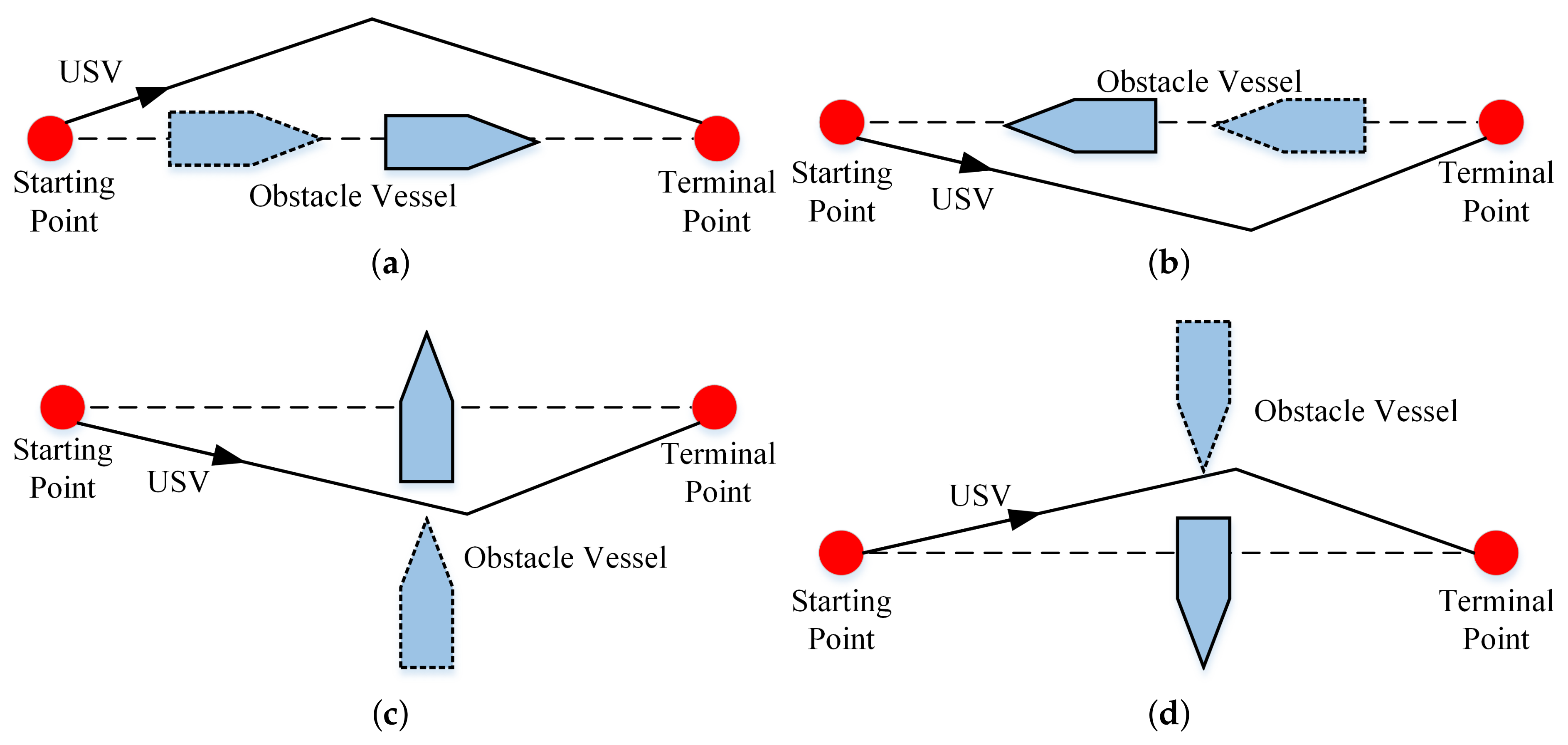
When the USV is sailing in the sea, it is usually necessary to follow certain rules to avoid the collision risk between the USV and obstacles. In the International Regulations for Preventing Collisions at Sea (COLREGs) formulated by the International Maritime Organization (IMO), the rules for avoiding collisions are given in the case of head-on, crossing and overtaking. Figure 5 is the schematic diagram of the three encounter situations.

In Figure 5, the USV sails from the starting point to the terminal point, and the blue vessel is the obstacle vessel encountered, in which the vessel shape with a solid edge represents the current position of the obstacle vessel, and the vessel shape with a dashed edge represents the position of the obstacle vessel at the last moment, from which the sailing trend of the obstacle vessel can be seen. The course of the USV is the sailing direction, and the course difference between the USV and the obstacle vessel starts from the USV course. The rules are described as follows:

(a)

Overtaking situation: when the course difference between the USV and the obstacle vessel is within [0${}^{\circ }$, 45${}^{\circ }$] and [315${}^{\circ }$, 360${}^{\circ }$], if the velocity of the USV is higher than that of the encountering vessel, then the USV turns left to pass the obstacle vessel.

(b)

Head-on situation: if the course difference is within [165${}^{\circ }$, 195${}^{\circ }$], the USV turns right to avoid the obstacle vessel.

(c)

Crossing situation: if the course difference is within [45${}^{\circ }$, 165${}^{\circ }$], the obstacle vessel crosses on the starboard side of the USV, then the USV turns right; if the course difference is within [195${}^{\circ }$, 315${}^{\circ }$], the obstacle vessel crosses on the port side of the USV, then the USV turns left.

4. The Dynamic Collision Avoidance Algorithm for the USV

4.1. Cuckoo Search Algorithm

In the cuckoo search algorithm, population updating is used to find the optimal nest location for oviposition behavior. There are two methods to generate new solutions: one is to update the nest position based on Levy flight; the another is to randomly search for a new location after the host bird abandons the nest after finding foreign eggs based on a certain probability [39].

In the cuckoo search (CS) algorithm, after the initial position is generated randomly, the current generation of a bird’s nest position is updated through Levy flight, and its formula is as follows:

$$\begin{array}{c}\hfill x_{t+1,i}=x_{t,i}+{\alpha }_c\oplus L\left(\lambda \right)·(x_{t,i}-x_{t,best})\end{array}$$

(18)

where $x_{t,i}$ is the i-nest in the t-generation population, $x_{t,best}$ is the optimal nest location in the population, and ${\alpha }_c$ is the step-size control factor, which is determined by the scale of the problem to be solved. $L\left(\lambda \right)$ follows the Levy probability distribution $L\left(\lambda \right)\sim u^{-\lambda }$. Next, some of the nest positions are eliminated according to the discovery probability $P_a$, and a new location is generated by using the preferred random walk method with

$$\begin{array}{c}\hfill x_{t+1,i}=x_{t,i}+r(x_{t,j}-x_{t,k}),\end{array}$$

(19)

where r is a random number evenly distributed between [0, 1], and $x_{t,j}$ and $x_{t,k}$ are two different random positions from the population.

4.2. Improved Cuckoo Search Algorithm

4.2.1. Adaptive Step-Size

In the CS algorithm, due to the strong randomness of Levy flight and the control factor of control flight step-size being a fixed value, it is easy to fly over the optimal solution in the optimization process and affect the convergence performance of the algorithm [40]. In this paper, through the analysis of the update strategy, the adaptive step-size adjustment mode is adopted by

$$\begin{array}{c}\hfill {\alpha }_c=\left(\frac{{\alpha }_{cmax}-{\alpha }_{cmin}}{1+exp(3·\gamma ·\frac{t}{T}-\gamma )}+{\alpha }_{cmin}\right)\end{array}$$

(20)

where $a_{cmax}$ and $a_{cmin}$ are the maximum and minimum of the step size, $\gamma$ can be used to adjust the decreasing rate, and t and T are the current iteration number and the total iteration number, respectively. Through (20), the flight step-size is larger in the early stage of iteration, which can fully search the solution space and determine the area where the optimal solution is located as soon as possible. With the increase in the iteration number, ${\alpha }_c$ gradually decreases, and local exploration can be carried out to improve the search accuracy and speed up the convergence.

4.2.2. Mutation and Crossover Operation

In the process of updating the CS algorithm, the diversity of individuals will be reduced and the global search ability will be poor. At this time, it is easy to fall into the local optimum and affect the convergence performance of the algorithm. Therefore, mutation and crossover operations are introduced in this paper. By randomly selecting three nests in the current nest population, the individual differences are used to generate a new intermediate nest position, and then the intermediate nest is crossed with the target nest to be replaced with a certain probability. The dimension variables are combined to generate a new nest position. The variation equation is as follows:

$$\begin{array}{c}\hfill y_{t,i}=x_{t,r1}+K·(x_{t,r2}-x_{t,r3})\end{array}$$

(21)

where the subscripts $r1$, $r2$ and $r3$ are three random numbers randomly selected within the population, which are not equal to each other and not equal to the i value of the current operator, and K is the scaling factor, which is between [0, 1]. The intermediate position $y_{t,i}$ is generated by three randomly selected bird’s nests, so that $y_{t,i}$ and current target position $x_{t,i}$ are crossed according to the crossing probability to generate a new bird’s nest individual $u_{i,j}$. The crossover operation equation is as follows:

$$\begin{array}{c}\hfill u_{i,j}=\left\{\begin{array}{c}{y}_{i,j}rand<P_{CR}\mathrm{or}j=j_{\mathit{rand}}\hfill \\ x_{i,j}other\hfill \end{array}\right.\end{array}$$

(22)

where $rand$ is the random number between [0, 1], $P_{CR}$ is the crossover probability, $j_{rand}$ is the random index value in [1, D] and D is the dimension number. The better dimension variables of two individuals can be retained in a new individual by cross-recombination between the intermediate individual and the target individual, so that the updated nest location is better.

By introducing mutation and crossover strategies, the algorithm can use the large differences between individuals to generate bird’s nest individuals with strong diversity in the early stage of iteration, so as to avoid falling into the local optimal situation, and strengthen the global search ability. In the process of convergence to the global optimum, these strategies enhance the local search ability.

4.2.3. Steps of the Improved Algorithm

The steps of the improved cuckoo search (ICS) algorithm are as follows:

• Step 1: The number T of iterations, population number N and discovery probability $P_a$, scaling factor K and crossover probability $P_{CR}$ are set and the positions of N nests are initialized randomly at the same time;
• Step 2: The population is updated using (18) with the adaptive step strategy, the individuals before and after updating are compared and the better solution is selected for retention;
• Step 3: According to the discovery probability $P_a$, some nests are eliminated, and the same number of new nests are generated by random walk according to (19);
• Step 4: According to (21) and (22), the nest position is mutated and crossed, and the better new individuals are reserved for the next iteration;
• Step 5: The position of the optimal solution in the population is selected, and whether the algorithm satisfies the termination condition is detected. If it is satisfied, the optimal solution will be output. If not, it will jump to Step 2.

4.3. Fitness Function Based on Collision Avoidance Model

Based on the collision avoidance model, the fitness function of the CS algorithm can be determined. According to (12), the USV can escape from the collision domain by changing course and velocity, so its fitness function can be expressed as

$$\begin{array}{c}\hfill f(\Delta v_U,\Delta \alpha )=k_1\left|\Delta v_U\right|+k_2\left|\Delta \alpha \right|\end{array}$$

(23)

where $f(\Delta v_U,\Delta \alpha )$ represents the sum of course variation $\Delta \alpha$ and velocity variation $\Delta v_U$ in the optimization process, and the variation constraint conditions are shown in

$$\begin{array}{c}\hfill \left\{\begin{array}{ccc}& \frac{sin\phi }{v_{UO}}\Delta v_U+\frac{v_{U}cos\phi }{v_{UO}}\Delta \alpha \ge {\mu }_1-\gamma \hfill & \gamma \ge 0\\ & \frac{sin\phi }{v_{UO}}\Delta v_U+\frac{v_{U}cos\phi }{v_{UO}}\Delta \alpha \le -{\mu }_2-\gamma \hfill & \gamma <0\end{array}\right..\end{array}$$

(24)

In the process of collision avoidance, under the condition that the USV can escape from the collision domain and meet the constraints of the collision avoidance rules, the USV sails in pursuit of a smaller attitude change and smooth motion, then the change in course and velocity should be as small as possible when seeking a collision avoidance strategy. In other words, the smaller value of fitness in the optimization process indicates the better position of the individual. The weight coefficients $k_1$ and $k_2$ are used to give priority to the adjustment of $\Delta \alpha$ and $\Delta v_U$. If the value of $k_1$ makes the value of $k_1$$\left|\Delta v_U\right|$ larger when adjusting the velocity, the course should be adjusted first. If $k_2$ makes $k_2$$\left|\Delta \alpha \right|$ larger when adjusting the course, the velocity should be adjusted first. Since it is more effective to adjust the course for collision avoidance, the adjustment of the course will be given priority in this paper.

4.4. Parameter Selection of Improved Algorithm

Considering that the CS algorithm needs to find the optimal solutions of $\Delta \alpha$ and $\Delta v_U$, the search space dimension is set to 2. The parameters of the ICS algorithm proposed in this paper include population number N, crossover probability $P_{CR}$, scaling factor K and detection probability $P_a$. The detection probability $P_a$ of the CS algorithm is generally 0.25 [34]. The population number N has a direct impact on the diversity of the nest position. If N is small, the algorithm converges quickly, but the probability of the algorithm falling into local optimization will also increase. Conversely, if N is set too large, the diversity of the nest position will increase, but it will increase the amount of calculation and reduce the convergence speed. For the crossover probability $P_{CR}$, it also has a great impact on the diversity of the population. When its value is large, it is easy to guarantee the diversity of the population, and the algorithm can easily find the optimal solution. Conversely, the change in the nest position is less, which is conducive to the stable search of the algorithm, but it is possible to fall into local optimization. The scaling factor K reflects the influence on the nest position offset. A larger K makes the nest position offset larger, which is convenient for the algorithm to find the potential solution in a large range. Conversely, the convergence speed can be improved, but this also makes the algorithm easily fall into local optimization. According to the above description, the N, $P_{CR}$ and K need to be properly selected according to the solution problem.

5. Collision Avoidance Trajectory Tracking Control

5.1. Structure of Collision Avoidance Controller

Figure 6 illustrates the principle of the collision avoidance controller, which combines the collision avoidance algorithm with the tracking controller. The sensor collects the environment and USV status information and then transmits it to the collision avoidance algorithm. The evasion trajectory is generated by the collision avoidance algorithm and used as the tracking trajectory of the tracking controller. Finally, the collision avoidance control of the USV is realized.

It is difficult for the tracking controller to accurately track the desired trajectory in the control cycle, so the collision avoidance algorithm needs to re-plan the trajectory according to the USV state and environmental information, as shown in Figure 7. As can be seen from Figure 7, the USV starts to sail from the point of A and plans the evasion trajectory of $A{B}_0$. However, due to the tracking error of the tracking controller, it only reaches the B position; that is, the actual trajectory is $AB$. The evasion trajectory $B{C}_0$ is planned again to compensate for the tracking error. The red solid line is the actual trajectory.

5.2. USV Model

The USV model is described as follows [41,42]:

$$\begin{array}{c}\hfill \left\{\begin{array}{c}\dot{x}=ucos\psi -vsin\psi \hfill \\ \dot{y}=usin\psi +vcos\psi \hfill \\ \dot{\psi }=r\hfill \\ \dot{u}=\frac{m_{22}}{m_{11}}vr-\frac{d_{11}}{m_{11}}u+\frac{1}{m_{11}}{\tau }_u\hfill \\ \dot{v}=-\frac{m_{11}}{m_{22}}ur-\frac{d_{22}}{m_{22}}v\hfill \\ \dot{r}=\frac{m_{11}-m_{22}}{m_{33}}uv-\frac{d_{33}}{m_{33}}r+\frac{1}{m_{33}}{\tau }_r\hfill \end{array}\right.,\end{array}$$

(25)

where $(x,y,\psi )$ denotes the surge displacement, sway displacement and yaw angle. $(u,v,r)$ denotes the velocities of surge, sway and yaw directions. The control inputs are surge force ${\tau }_u$ and yaw moment ${\tau }_r$. $m_{ii}$ and $d_{ii}$ are the vessel inertia coefficients and damping coefficients.

5.3. Tracking Controller Design

The position tracking error is

$$\left\{\begin{array}{c}\hfill x_e=x-x_d\\ \hfill y_e=y-y_d\end{array}\right..$$

(26)

The derivation of time t on both sides of (26) can be obtained

$$\left[\begin{array}{c}{\dot{x}}_e\hfill \\ {\dot{y}}_e\hfill \end{array}\right]=R\left(\psi \right)\left[\begin{array}{c}u\hfill \\ v\hfill \end{array}\right]-\left[\begin{array}{c}{\dot{x}}_d\hfill \\ {\dot{y}}_d\hfill \end{array}\right],$$

(27)

with

$$R\left(\psi \right)=\left[\begin{array}{cc}cos\psi & -sin\psi \\ sin\psi & cos\psi \end{array}\right].$$

For u and v, the virtual control laws ${\alpha }_u$ and ${\alpha }_v$ with $\mathrm{\Lambda }=\sqrt{x_e^2+y_e^2+\nabla }$ are

$$\left[\begin{array}{c}{\alpha }_u\hfill \\ {\alpha }_v\hfill \end{array}\right]=R{\left(\psi \right)}^{-1}\left[\begin{array}{c}{\dot{x}}_d-\kappa x_e/\mathrm{\Lambda }\hfill \\ {\dot{y}}_d-\kappa y_e/\mathrm{\Lambda }\hfill \end{array}\right],$$

(28)

where $\kappa >0$ and $\nabla >0$. When $u_{eg}=u-{\alpha }_u$,$v_{eg}=v-{\alpha }_v$, then

$$\left[\begin{array}{c}{\dot{x}}_e\hfill \\ {\dot{y}}_e\hfill \end{array}\right]=R\left(\psi \right)\left[\begin{array}{c}{u}_{eg}\hfill \\ v_{eg}\hfill \end{array}\right]-\left[\begin{array}{c}\kappa x_e/\mathrm{\Lambda }\hfill \\ \kappa y_e/\mathrm{\Lambda }\hfill \end{array}\right].$$

(29)

When $u_{eg}\to 0$, $v_{eg}\to 0$, (29) is updated to

$$\left[\begin{array}{c}{\dot{x}}_e\hfill \\ {\dot{y}}_e\hfill \end{array}\right]=-\left[\begin{array}{c}\kappa x_e/\mathrm{\Lambda }\hfill \\ \kappa y_e/\mathrm{\Lambda }\hfill \end{array}\right].$$

(30)

Consider the following candidate Lyapunov function as

$$V_0=\frac{1}{2}{x}_e^2+\frac{1}{2}{y}_e^2.$$

(31)

Deriving from (31) we can obtain

$${\dot{V}}_0=x_e^{}{\dot{x}}_e^{}+y_e^{}{\dot{y}}_e^{}=-\kappa \left(x_e^2+y_e^2\right)/\mathrm{\Lambda }.$$

(32)

According to (32) and (30), when $\underset{t\to \infty }{lim}{\dot{V}}_0\le 0$, the position error converges to zero gradually.

The PID controller is introduced as the tracking controller, and its control law is as follows

$$\begin{array}{c}\hfill \mathbf{u}=K_p\mathrm{\Gamma }\left(t\right)+K_i{\int }_0^t\mathrm{\Gamma }\left(t\right)dt+K_d\dot{\mathrm{\Gamma }}\left(t\right),\end{array}$$

(33)

where $\mathrm{\Gamma }={\left[u_{eg},v_{eg}\right]}^T$, and the proportional coefficient, integral coefficient and differential coefficient of the PID controller are $K_p=diag\left(K_{pu},K_{pv}\right)$, $K_i=diag\left(K_{iu},K_{iv}\right)$ and $K_d=diag\left(K_{du},K_{dv}\right),$ respectively.

6. Simulation of Dynamic Collision Avoidance Algorithm

On a computer with a CPU of 2.93 HZ, Matlab 2014a was used for algorithm simulation to test the feasibility of the designed autonomous collision avoidance control algorithm based on the improved CS algorithm.

6.1. Simulation Verification of Improved CS Algorithm

In order to verify the effectiveness of the improved CS (ICS) algorithm, four sets of test functions were used to test the convergence speed and optimization accuracy of the algorithm. Among them, the $f_1$ function is a unimodal function used to verify the convergence speed of the algorithm; $f_2$, $f_3$ and $f_4$ are multimodal functions with many local extremum points, which are used to verify the optimization accuracy of the algorithm. The ICS algorithm was compared with the standard CS algorithm and particle swarm optimization (PSO). Parameters were set as follows: population number N = 30, search space dimension was 2, $P_{CR}$ = 0.2, K = 0.55 was in the improved CS algorithm, detection probability $P_a$ = 0.25 was in the CS algorithm, $c_1=c_2=2$ was in the PSO algorithm and inertia weight w decreased linearly from 0.9 to 0.4 [43]. Test functions are shown in

Table 1. Test functions.

Function Name	Function Equation	Search Scope	Optimal Value
Sphere	$f_1={\displaystyle \sum _{i=1}^D}{x}_i^2$	[−5.12, 5.12]	0
Ackley	$\begin{array}{c}{f}_2=-20exp(-0.2\sqrt{{\displaystyle \sum _{i=1}^D}\frac{x_i^2}{D}})-\hfill \\ exp({\displaystyle \sum _{i=1}^D}cos(2\pi x_i/D))+20+e\hfill \end{array}$	[−32, 32]	0
Girewank	$f_3=\frac{1}{4000}{\displaystyle \sum _{i=1}^D}{x}_i^2-{\displaystyle \prod _{i=1}^D}cos(\frac{x_i}{\sqrt{i}})+1$	[−600, 600]	0
Schaffer	$f_4=0.5+\frac{{(sin\sqrt{x_1^2+x_2^2})}^2-0.5}{{(1+0.001(x_1^2+x_2^2))}^2}$	[−10, 10]	0

.

To verify the algorithm by numerical simulation, the test functions were used. Their fitness curve and simulation results are shown in Figure 8 and

Table 2. Simulation results of test functions.

Function	Algorithm	Optimal Solution	Worst Solution	Average Value
Sphere	PSO	1.1812 × 10${}^{-8}$	8.6634 × 10${}^{-7}$	2.1987 × 10${}^{-7}$
	CS	1.1803 × 10${}^{-6}$	1.3057 × 10${}^{-5}$	5.0170 × 10${}^{-6}$
	ICS	1.7019 × 10${}^{-19}$	2.8024 × 10${}^{-18}$	1.1439 × 10${}^{-18}$
Ackley	PSO	8.9423 × 10${}^{-7}$	5.4106 × 10${}^{-5}$	2.0311 × 10${}^{-5}$
	CS	2.2135 × 10${}^{-8}$	2.6034 × 10${}^{-6}$	4.1700 × 10${}^{-7}$
	ICS	8.8818 × 10${}^{-16}$	2.2204 × 10${}^{-14}$	8.7041 × 10${}^{-15}$
Girewank	PSO	9.6883 × 10${}^{-4}$	0.0494	0.0198
	CS	0.0020	0.0272	0.0115
	ICS	0	8.1406 × 10${}^{-12}$	8.6685 × 10${}^{-13}$
Schaffer	PSO	2.4826 × 10${}^{-9}$	0.0097	0.0058
	CS	8.4831 × 10${}^{-8}$	0.0097	0.0051
	ICS	5.7732 × 10${}^{-15}$	1.6292 × 10${}^{-6}$	3.2832 × 10${}^{-7}$

.

Through the verification of test functions and the results in Figure 8 and Table 2, it can be seen that the ICS algorithm improves the convergence speed and accuracy by adjusting the flight step-size adaptively. Mutation and crossover operations were introduced to avoid the population falling into local optima and enhance the ability of global optimization. Compared with the standard CS and PSO algorithms, the ICS algorithm performs better in convergence speed, accuracy and global optimization ability, and can meet the calculation requirements of the collision avoidance strategy when applied to USV dynamic collision avoidance.

6.2. Simulation Verification for Collision Avoidance

In order to verify the collision avoidance ability of the USV in a multi-obstacle scene, the real electronic chart in Figure 9 was taken as the simulation scene.

Table 3. Data for multiple dynamic obstacle avoidance.

	Starting Point	Target Point	Direction	Velocity
USV	(0, 280)	(900, 800)	90${}^{\circ }$	30
Obstacle 1	(590, 120)		270${}^{\circ }$	(−17, 0)
Obstacle 2	(500, −80)		0${}^{\circ }$	(0, 10)
Obstacle 3	(1100, 520)		270${}^{\circ }$	(−12, 0)
Obstacle 4	(760, 1050)		180${}^{\circ }$	(0, −10)

shows the motion information of the USV and obstacles, with the coordinate unit m and velocity unit kn. The numerical simulation was carried out on the Lanxin USV of Dalian Maritime University, for which principal parameters can be found in [33]. The initial conditions of the USV were $\{x,y,\psi ,u,v,r\}\left(0\right)$ = {0 m, 280 m, 0 rad, 0 m/s, 0 m/s, 0 rad/s}. The control parameters were selected as $\kappa =1,\nabla =1$, $K_p=diag\left(1.0\times {10}^3,1.0\times {10}^3\right)$, $K_i=diag\left(0.3\times {10}^3,0.3\times {10}^3\right)$ and $K_d=diag\left(20,20\right)$.

The collision avoidance simulation for the USV in a multi-obstacle scene is shown in Figure 10, in which the blue trajectory is the collision avoidance route of the USV, and the other trajectories are those of dynamic obstacles.

In Figure 10, the USV detects whether there is an obstacle at any time during its voyage. In Figure 10a, the USV detects that it meets obstacle 1 and completes the obstacle avoidance by maintaining course −39${}^{\circ }$. In Figure 10b, the USV detects the crossing obstacle 2, and the USV turns to the course 31${}^{\circ }$ to complete the obstacle avoidance with a velocity of 6 m/s and a single calculation time of 0.078 s. In Figure 10c, crossing obstacle 3 is detected, the USV turns to the course 16.49${}^{\circ }$, and the velocity is 7 m/s to complete the obstacle avoidance with a single calculation time of 0.076 s. In Figure 10d, the USV crosses with obstacle 4, and the USV turns to the course 84.61${}^{\circ }$ to complete the collision avoidance for obstacle 4 with a single calculation time of 0.077 s. The collision avoidance behavior in the above process follows the collision avoidance rules. In Figure 10e,f, after the USV completes the collision avoidance for obstacle 4, it adjusts the course and velocity and sails to the target point.

Figure 11a shows the input of the controller. Under the control inputs, the final control output of the USV is shown in Figure 11b. It can be seen that the controller can better follow the velocity and course guidance instructions output with the collision avoidance algorithm.

According to the expected course and velocity calculated by the collision avoidance algorithm, the USV will adjust to the expected motion attitude according to its own motion performance constraints, and calculate the expected attitude change at the next moment in real time according to the adjusted motion state parameters and position information, so as to realize real-time collision avoidance. From the above simulation, it can be seen that the collision avoidance algorithm designed in this paper can make the USV complete the obstacle avoidance safely and quickly.

7. Conclusions

Aiming at the autonomous dynamic collision avoidance problem for a USV, a collision avoidance control method based on an improved CS algorithm was proposed. Firstly, according to the different aspect ratios of obstacle contours, these are represented by circle and ellipse collision avoidance models. In the process of collision avoidance, the constraints of collision avoidance rules are integrated to ensure the safety of the USV during a voyage. Secondly, the CS algorithm was improved by using the adaptive step-size control factor, so as to dynamically adjust the flight step-size and improve the search ability; by introducing a mutation and crossover strategy, the diversity of the population and local optimization ability were strengthened. The improved CS algorithm, standard CS algorithm and PSO algorithm were simulated and verified. By comparison, the improved CS algorithm shows great improvement in the convergence speed and optimization accuracy, and it can quickly solve the collision avoidance strategy in the process of collision avoidance. Through experiments for electronic chart scene simulation, it was verified that the algorithm designed can make the USV complete autonomous dynamic collision avoidance safely and quickly in multi-dynamic obstacle scenes, which provides a feasible and effective engineering application method for autonomous dynamic collision avoidance of a USV. In future research, it will be necessary to further combine the relevant contents of COLREGs with a collision avoidance controller to ensure the sailing safety of the USV.

References

1. Liu, Z.; Zhang, Y.; Yu, X.; Yuan, C. Unmanned surface vehicles: An overview of developments and challenges. Annu. Rev. Control 2016, 41, 71–93. [Google Scholar] [CrossRef]
2. Felski, A.; Zwolak, K. The Ocean-Going Autonomous Ship-Challenges and Threats. J. Mar. Sci. Eng. 2020, 8, 41. [Google Scholar] [CrossRef] [Green Version]
3. Zhou, C.H.; Gu, S.D.; Wen, Y.Q.; Du, Z.; Xiao, C.S.; Huang, L.; Zhu, M. The review unmanned surface vehicle path planning: Based on multi-modality constraint. Ocean. Eng. 2020, 200, 107043. [Google Scholar] [CrossRef]
4. Kuwata, Y.; Wolf, M.T.; Zarzhitsky, D.; Huntsberger, T.L. Safe Maritime Autonomous Navigation With COLREGS, Using Velocity Obstacles. IEEE J. Ocean. Eng. 2013, 39, 110–119. [Google Scholar] [CrossRef]
5. Tang, P.; Zhang, R.; Liu, D.; Huang, L.; Liu, G.; Deng, T. Local reactive obstacle avoidance approach for high-speed unmanned surface vehicle. Ocean Eng. 2015, 106, 128–140. [Google Scholar] [CrossRef]
6. Song, A.L.; Su, B.Y.; Dong, C.Z.; Shen, D.W.; Xiang, E.Z.; Mao, F.P. A two-level dynamic obstacle avoidance algorithm for unmanned surface vehicles. Ocean Eng. 2018, 170, 351–360. [Google Scholar] [CrossRef]
7. Xiong, C.K.; Lu, D.; Zeng, Z.; Lian, L.; Yu, C.Y. Path Planning of Multiple Unmanned Marine Vehicles for Adaptive Ocean Sampling Using Elite Group-Based Evolutionary Algorithms. J. Intell. Robot. Syst. 2020, 99, 875–889. [Google Scholar] [CrossRef]
8. Sun, X.; Wang, G.; Fan, Y.; Mu, D.; Qiu, B. A Formation Autonomous Navigation System for Unmanned Surface Vehicles With Distributed Control Strategy. IEEE Trans. Intell. Transp. Syst. 2020, 22, 2834–2845. [Google Scholar] [CrossRef]
9. Sun, X.J.; Wang, G.F.; Fan, Y.S.; Mu, D.D.; Qiu, B.B. Fast Collision Avoidance Method Based on Velocity Resolution for Unmanned Surface Vehicle. In Proceedings of the 2019 31st Chinese Control and Decision Conference (CCDC 2019), Nanchang, China, 3–5 June 2019; pp. 4822–4827. [Google Scholar]
10. Guo, X.H.; Ji, M.J.; Zhao, Z.W.; Wen, D.S.; Zhang, W.D. Global path planning and multi-objective path control for unmanned surface vehicle based on modified particle swarm optimization (PSO) algorithm. Ocean. Eng. 2020, 216, 107693. [Google Scholar] [CrossRef]
11. Xia, G.Q.; Han, Z.W.; Zhao, B.; Wang, X.W. Unmanned Surface Vehicle Collision Avoidance Trajectory Planning in an Uncertain Environment. IEEE Access 2020, 8, 207844–207857. [Google Scholar] [CrossRef]
12. Li, Y.; Zheng, J. Real-time collision avoidance planning for unmanned surface vessels based on field theory. ISA Trans. 2020, 106, 233–242. [Google Scholar] [CrossRef]
13. Xu, X.L.; Pan, W.; Huang, Y.B.; Zhang, W.D. Dynamic Collision Avoidance Algorithm for Unmanned Surface Vehicles via Layered Artificial Potential Field with Collision Cone. J. Navig. 2020, 73, 1306–1325. [Google Scholar] [CrossRef]
14. Chen, Y.L.; Bai, G.Q.; Zhan, Y.; Hu, X.Y.; Liu, J. Path Planning and Obstacle Avoiding of the USV Based on Improved ACO-APF Hybrid Algorithm With Adaptive Early-Warning. IEEE Access 2021, 9, 40728–40742. [Google Scholar] [CrossRef]
15. Guardeno, R.; Lopez, M.J.; Sanchez, J.; Consegliere, A. AutoTuning Environment for Static Obstacle Avoidance Methods Applied to USVs. J. Mar. Sci. Eng. 2020, 8, 300. [Google Scholar] [CrossRef]
16. Wang, D.; Zhang, J.; Jin, J.C.; Mao, X.P. Local Collision Avoidance Algorithm for a Unmanned Surface Vehicle Based on Steering Maneuver Considering COLREGs. IEEE Access 2021, 9, 49233–49248. [Google Scholar] [CrossRef]
17. Liang, C.L.; Zhang, X.K.; Watanabe, Y.; Deng, Y.J. Autonomous Collision Avoidance of Unmanned Surface Vehicles Based on Improved A Star And Minimum Course Alteration Algorithms. Appl. Ocean. Res. 2021, 113, 102755. [Google Scholar] [CrossRef]
18. Sang, H.Q.; You, Y.S.; Sun, X.J.; Zhou, Y.; Liu, F. The hybrid path planning algorithm based on improved A* and artificial potential field for unmanned surface vehicle formations. Ocean. Eng. 2021, 223, 108709. [Google Scholar] [CrossRef]
19. Tan, G.G.; Zou, J.; Zhuang, J.Y.; Wan, L.; Sun, H.B.; Sun, Z.Y. Fast marching square method based intelligent navigation of the unmanned surface vehicle swarm in restricted waters. Appl. Ocean. Res. 2020, 95, 102018. [Google Scholar] [CrossRef]
20. Polvara, R.; Sharma, S.; Wan, J.; Manning, A.; Sutton, R. Obstacle Avoidance Approaches for Autonomous Navigation of Unmanned Surface Vehicles. J. Navig. 2018, 71, 241–256. [Google Scholar] [CrossRef] [Green Version]
21. Woo, J.; Kim, N. Collision avoidance for an unmanned surface vehicle using deep reinforcement learning. Ocean. Eng. 2020, 199, 107001. [Google Scholar] [CrossRef]
22. Song, L.F.; Chen, H.J.; Xiong, W.H.; Dong, Z.P.; Mao, P.X.; Xiang, Z.Q.; Hu, K. Method of Emergency Collision Avoidance for Unmanned Surface Vehicle (usv) Based on Motion Ability Database. Pol. Marit. Res. 2019, 26, 55–67. [Google Scholar] [CrossRef] [Green Version]
23. Xia, G.Q.; Han, Z.W.; Zhao, B.; Wang, X.W. Local Path Planning for Unmanned Surface Vehicle Collision Avoidance Based on Modified Quantum Particle Swarm Optimization. Complexity 2020, 2020, 3095426. [Google Scholar] [CrossRef]
24. Lazarowska, A. Ship’s Trajectory Planning for Collision Avoidance at Sea Based on Ant Colony Optimisation. J. Navig. 2015, 68, 291–307. [Google Scholar] [CrossRef] [Green Version]
25. Lazarowska, A. Swarm Intelligence Approach to Safe Ship Control. Pol. Marit. Res. 2015, 22, 34–40. [Google Scholar] [CrossRef] [Green Version]
26. Wang, H.J.; Guo, F.; Yao, H.F.; He, S.S.; Xu, X. Collision Avoidance Planning Method of USV Based on Improved Ant Colony Optimization Algorithm. IEEE Access 2019, 7, 52964–52975. [Google Scholar] [CrossRef]
27. Rakhshani, H.; Rahati, A. Snap-drift cuckoo search: A novel cuckoo search optimization algorithm. Appl. Soft Comput. 2017, 52, 771–794. [Google Scholar] [CrossRef]
28. Yang, X.S.; Deb, S. Cuckoo search: Recent advances and applications. Neural Comput. Appl. 2014, 24, 169–174. [Google Scholar] [CrossRef] [Green Version]
29. Hosseininejad, S.; Dadkhah, C. Mobile robot path planning in dynamic environment based on cuckoo optimization algorithm. Int. J. Adv. Robot. Syst. 2019, 16, 172988141983957. [Google Scholar] [CrossRef]
30. Mohanty, P.K. An intelligent navigational strategy for mobile robots in uncertain environments using smart cuckoo search algorithm. J. Ambient. Intell. Humaniz. Comput. 2020, 11, 6387–6402. [Google Scholar] [CrossRef]
31. Chen, P.; Huang, Y.; Mou, J.; van Gelder, P. Ship collision candidate detection method: A velocity obstacle approach. Ocean. Eng. 2018, 170, 186–198. [Google Scholar] [CrossRef]
32. Fan, Y.S.; Mu, D.D.; Zhang, X.K.; Wang, G.F.; Guo, C. Course keeping Control Based on Integrated Nonlinear Feedback for a USV with Pod-like Propulsion. J. Navig. 2018, 71, 878–898. [Google Scholar] [CrossRef]
33. Sun, X.J.; Wang, G.F.; Fan, Y.S. Model Identification and Trajectory Tracking Control for Vector Propulsion Unmanned Surface Vehicles. Electronics 2020, 9, 22. [Google Scholar] [CrossRef] [Green Version]
34. Yang, X.S.; Deb, S. Cuckoo Search via Levey Flights. In Proceedings of the 2009 World Congress on Nature & Biologically Inspired Computing (NABIC 2009), Coimbatore, India, 9–11 December 2009. [Google Scholar]
35. Zhang, M.Q.; Wang, H.; Cui, Z.H.; Chen, J.J. Hybrid multi-objective cuckoo search with dynamical local search. Memetic Comput. 2018, 10, 199–208. [Google Scholar] [CrossRef]
36. Liu, H.D.; Liu, Q.; Sun, R. Deterministic Vessel Automatic Collision Avoidance Strategy Evaluation Modeling. Intell. Autom. Soft Comput. 2019, 25, 789–804. [Google Scholar] [CrossRef]
37. Zhou, K.; Chen, J.H.; Liu, X. Optimal Collision-Avoidance Manoeuvres to Minimise Bunker Consumption under the Two-Ship Crossing Situation. J. Navig. 2018, 71, 151–168. [Google Scholar] [CrossRef]
38. Szlapczynski, R.; Szlapczynska, J. An analysis of domain-based ship collision risk parameters. Ocean. Eng. 2016, 126, 47–56. [Google Scholar] [CrossRef]
39. Ong, P.; Zainuddin, Z. Optimizing wavelet neural networks using modified cuckoo search for multi-step ahead chaotic time series prediction. Appl. Soft Comput. 2019, 80, 374–386. [Google Scholar] [CrossRef]
40. Ljouad, T.; Amine, A.; Rziza, M. A hybrid mobile object tracker based on the modified Cuckoo Search algorithm and the Kalman Filter. Pattern Recognit. 2014, 47, 3597–3613. [Google Scholar] [CrossRef]
41. Dong, W.; Guo, Y. Global time-varying stabilization of underactuated surface vessel. IEEE Trans. Autom. Control 2005, 50, 859–864. [Google Scholar] [CrossRef]
42. Fossen, T.I. Handbook of Marine Craft Hydrodynamics and Motion Control; John Wiley & Sons: New York, NY, USA, 2011. [Google Scholar]
43. Shi, Y. A Modified Particle Swarm Optimizer. In Proceedings of the IEEE World Congress on Computational Intelligence (Cat. No. 98TH8360), Anchorage, AK, USA, 4–9 May 1998. [Google Scholar]
Figure 1. The Lanxin USV at sea.
Applsci 11 09741 g001
Figure 2. Circular collision avoidance model.
Applsci 11 09741 g002
Figure 3. Ellipse obstacle avoidance model.
Applsci 11 09741 g003
Figure 4. Tangents of ellipse obstacle.
Applsci 11 09741 g004
Figure 5. Rule diagram of collision avoidance. (a) Overtaking situation; (b) Head-on situation; (c) Crossing situation on the starboard side of USV; (d) Crossing situation on the port side of USV.
Applsci 11 09741 g005
Figure 6. The collision avoidance controller.
Applsci 11 09741 g006
Figure 7. The actual and desired trajectories for collision avoidance.
Applsci 11 09741 g007
Figure 8. Fitness curves of test functions. (a) Sphere function; (b) Ackle function; (c) Girewank function; (d) Schaffer function.
Applsci 11 09741 g008
Figure 9. Chart scene.
Applsci 11 09741 g009
Figure 10. Multiple dynamic obstacle avoidance. (a) Encounter obstacle 1; (b) Encounter obstacle 2; (c) Encounter obstacle 3; (d) Encounter obstacle 4; (e) Leave obstacle 4; (f) Achieve the goal.
Applsci 11 09741 g010
Figure 11. Input and output results for the controller. (a) The input of the controller; (b) The final control output of USV.
Applsci 11 09741 g011