Article

Fast Performance Modeling across Different Database Versions Using Partitioned Co-Kriging

School of Computer Science and Technology, Xidian University, Xi’an 710071, China
*
Author to whom correspondence should be addressed.
Appl. Sci. 2021, 11(20), 9669; https://doi.org/10.3390/app11209669
Submission received: 3 September 2021 / Revised: 9 October 2021 / Accepted: 13 October 2021 / Published: 16 October 2021

Abstract

:
Database systems have a large number of configuration parameters that control functional and non-functional properties (e.g., performance and cost). Different configurations may lead to different performance values. To understand and predict the effect of configuration parameters on system performance, several learning-based strategies have been recently proposed. However, existing approaches usually assume a fixed database version such that learning has to be repeated once the database version changes. Repeating measurement and learning for each version is expensive and often practically infeasible. Instead, we propose the Partitioned Co-Kriging (PCK) approach that transfers knowledge from an older database version (source domain) to learn a reliable performance prediction model fast for a newer database version (target domain). Our method is based on the key observations that performance responses typically exhibit similarities across different database versions. We conducted extensive experiments under 5 different database systems with different versions to demonstrate the superiority of PCK. Experimental results show that PCK outperforms six state-of-the-art baseline algorithms in terms of prediction accuracy and measurement effort.

1. Introduction

Database systems are increasingly becoming more configurable [1,2]. The large number of configuration parameters can directly influence the functional and non-functional properties of database systems [3,4]. Performance (e.g., latency, throughput, and requests per second) is one of the most important non-functional properties as it directly affects user experience [5]. Appropriate configurations can improve the performance for database systems [2,6]. For example, the throughput difference between the best and worst configurations for Cassandra can be as high as 102.5% for a given workload [7]. To distinguish the optimal configuration, users are interested in knowing the consequences of changing the configuration parameters that are available to them. However, the exponentially growing configuration space and complex interactions among configuration parameters make it difficult to understand the performance of the system [8,9].
In recent years, learning-based approaches have become the mainstream to solve this problem. These methods often collect the performance measurements of only a limited set of configurations (called samples), then build a performance model with these samples, and use the model to predict the system performance of the unseen configurations [7,10,11,12,13,14]. In this way, performance can be predicted before a variant of the database system is configured and deployed.
Existing approaches usually focus on the performance modeling problem under a constant environment, including fixed hardware [11,14], workload [9,10], and database version [2,7]. We will concentrate on performance modeling for a newer database version in this work. In practice, previous performance prediction models often lead to high prediction error once the database version changes [15]. A new performance prediction model may need to be learned from scratch to meet the prediction accuracy requirements. However, the demand for high quality samples in learning-based methods contradicts the need for rapid acquisition of a new performance prediction model. Specifically, researchers often need a large number of samples to build a good performance prediction model [16]. However, the collection of samples requires a lot of time and resources [6,10], which makes the construction of the new performance model time-consuming and laborious.
Fortunately, performance models typically exhibit similarities across different database versions [17]. We introduce the concept of transfer learning into performance modeling for database systems. Similar to humans that learn from previous experience and transfer the knowledge learned to accomplish new tasks easier [18], here, knowledge about performance behavior observed in an older database can be reused effectively to learn models for a newer database with a lower cost. The problem is to identify the transferable knowledge and make use of them to ease learning of performance models.
In this paper, we propose a co-kriging-based performance prediction method to efficiently learn models by reusing information gained previously when database version changes. The challenge is to predict system performance with high accuracy while utilizing a small sample in target domain. As it takes time and effort to configure the database system and collect performance measurement data, it is desirable that the sample size is kept minimum. Co-kriging allows data on an auxiliary variable to be used to make up for an insufficient amount of data in undersampled case [19]. We regard the performance responses in older (source) and newer (target) database systems as the auxiliary variable and primary variable, respectively. The measurement data in source can facilitate building an accurate performance model in target by co-kriging with a small sample in target.
Further, Partitioned Co-Kriging (PCK) is proposed to better satisfy the assumption of co-kriging method. The assumption of co-kriging method is that the performance response is stationary [20]. The accuracy of performance model can increase obviously by applying co-kriging in several regions which performance responses are smooth. The partition of these smooth regions is regarded as transferable knowledge, and it can be obtained by clustering the measurement data in source domain.
In a nutshell, we regard the partition of smooth regions and the measurement data in source as transferable knowledge. Furthermore, the PCK is presented to make use of the transferable knowledge to fast construct performance models in target. Finally, we demonstrate that our PCK approach will enable accurate performance predictions by using only a small number of measurements in target domain. We evaluate our approach on five different database systems: MySQL, PostgreSQL, SQLite, Redis, and Cassandra.
In summary, our work makes the following contributions.
  • We perform a proof of concept that transferring the knowledge across different database versions using PCK can facilitate the fast performance modeling for a newer database version.
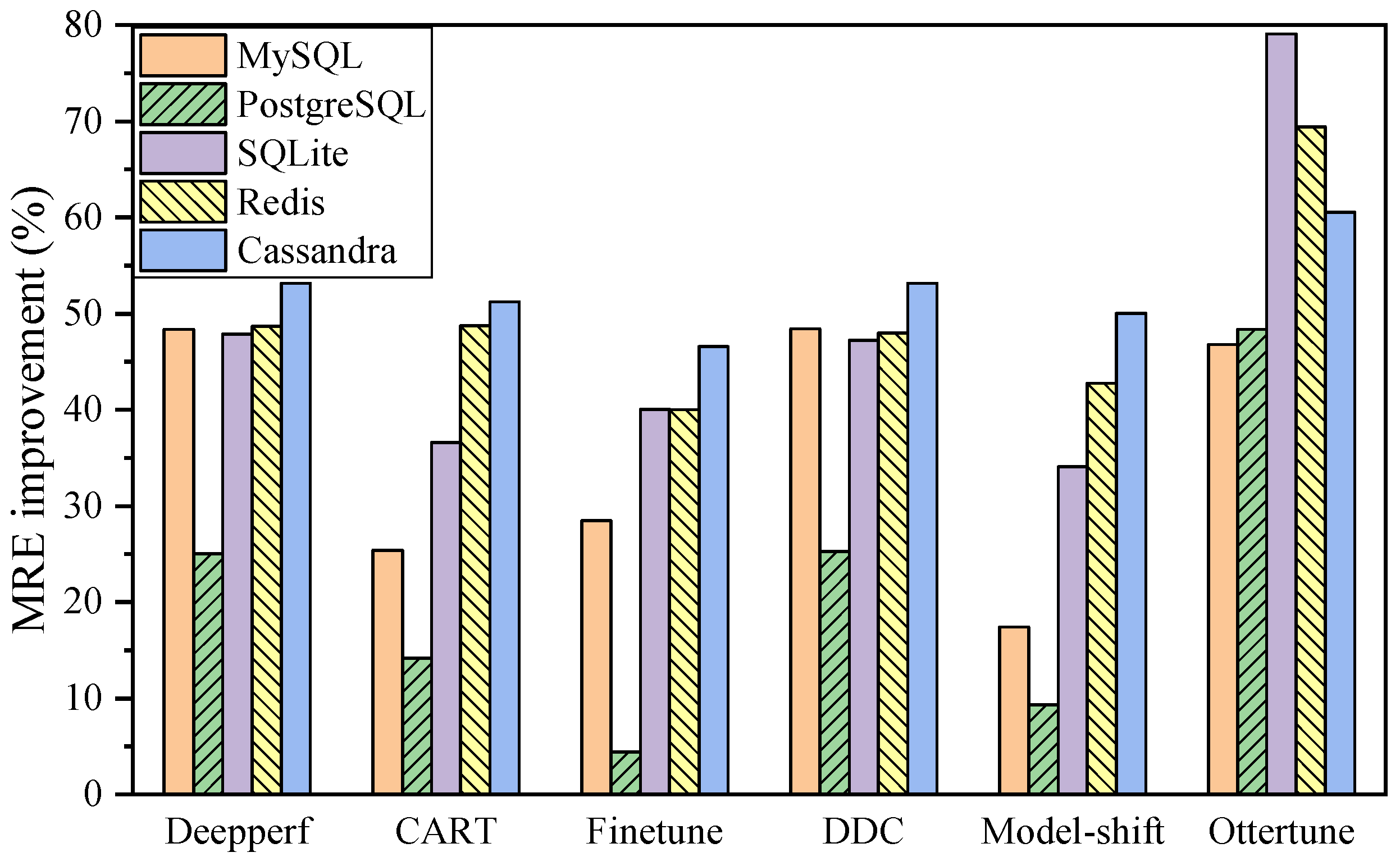
  • We verify the feasibility and validity of PCK through extensive experiments under different categories of database systems with different versions. Experimental results show that our proposal outperforms six state-of-the-art baseline algorithms by 30.73–60.83% on average.

2. Related Work

Researchers make an effort to understand the relationship of parameters and performance. Several performance prediction models [3,5,10,11,12,13,14,21,22,23] and tuning strategies [6,16,24,25,26,27,28,29,30,31] have been proposed to explore the relationship and recommend good configurations further.
Performance Prediction for Databases. The performance prediction methods fall into two major categories: analytical prediction models and learning-based prediction models. The first class of approaches require an in-depth analysis of the constraints on system performance, and the analysis models are given accordingly [24,25,26]. The latter class of approaches train prediction models using machine learning techniques, including GP regression [2,6,27,32], neural networks [7,10,28,29], CART [3,5,11,12,13,14], Fourier Learning [21,22], and so on.
Existing approaches usually assume a fixed environment such that the modeling/tuning process has to start from the scratch once the environment changes, which exacerbates the performance modeling problem. Therefore, transferring knowledge across environments to assist the modeling/tuning task has become a hot area of research in recent years.
Knowledge Transfer for Performance Prediction. The most relevant research to this paper is to transfer performance prediction models across environments.
To cope with the workload changes, OtterTune [2,32] reuses past experience to reduce the tuning cost for a new application. Rafiki [7] includes workload characteristics and the most impactful parameters directly in its surrogate model.
Valov et al. [33] analyzed different hardware platforms to understand the similarity on performance prediction. A simple linear regression model is used to transfer knowledge from a related environment to a target environment. Differently, there is another kind of approach that reuses source data with the hope to capture correlation between environments using learners such as GP Models [34].
Further, it is worth exploring why and when transfer learning works for performance modeling. Jamshidi et al. [17] combine many statistical and machine learning techniques to study this research question. Javidian et al. [35] exploit causal analysis to identify the key knowledge pieces that can be exploited for transfer learning.
Jamshidi et al. [15] propose a sampling strategy L2S, which is inspired by the research results in [17]. L2S extracts transferable knowledge from the source to drive the selection of more informative samples in the target environment.
Moreover, transfer learning can only be useful in cases where the source environment is similar to the target environment. BEETLE [36] focuses on the problem of whence to learn. A racing algorithm is applied to sequentially evaluate candidate environments to discover which of the available environments are best suited to be a source environment.
In this paper, we concentrate on transferring knowledge across different database versions. There are few relevant researches on this issue at present. The studies on version change scenario is the least among the three main environment change scenarios. The exploratory analysis [17] and causal analysis [35] give us insights into performance prediction across environment change, but no transfer scheme is given in these studies. BEETLE [36] places emphasis on identifying suitable sources to construct transfer learner. Other work [15,34] has made some discussion about the version change scenario, but they have not conducted in-depth research and experimental verification on this issue.

3. Problem Overview

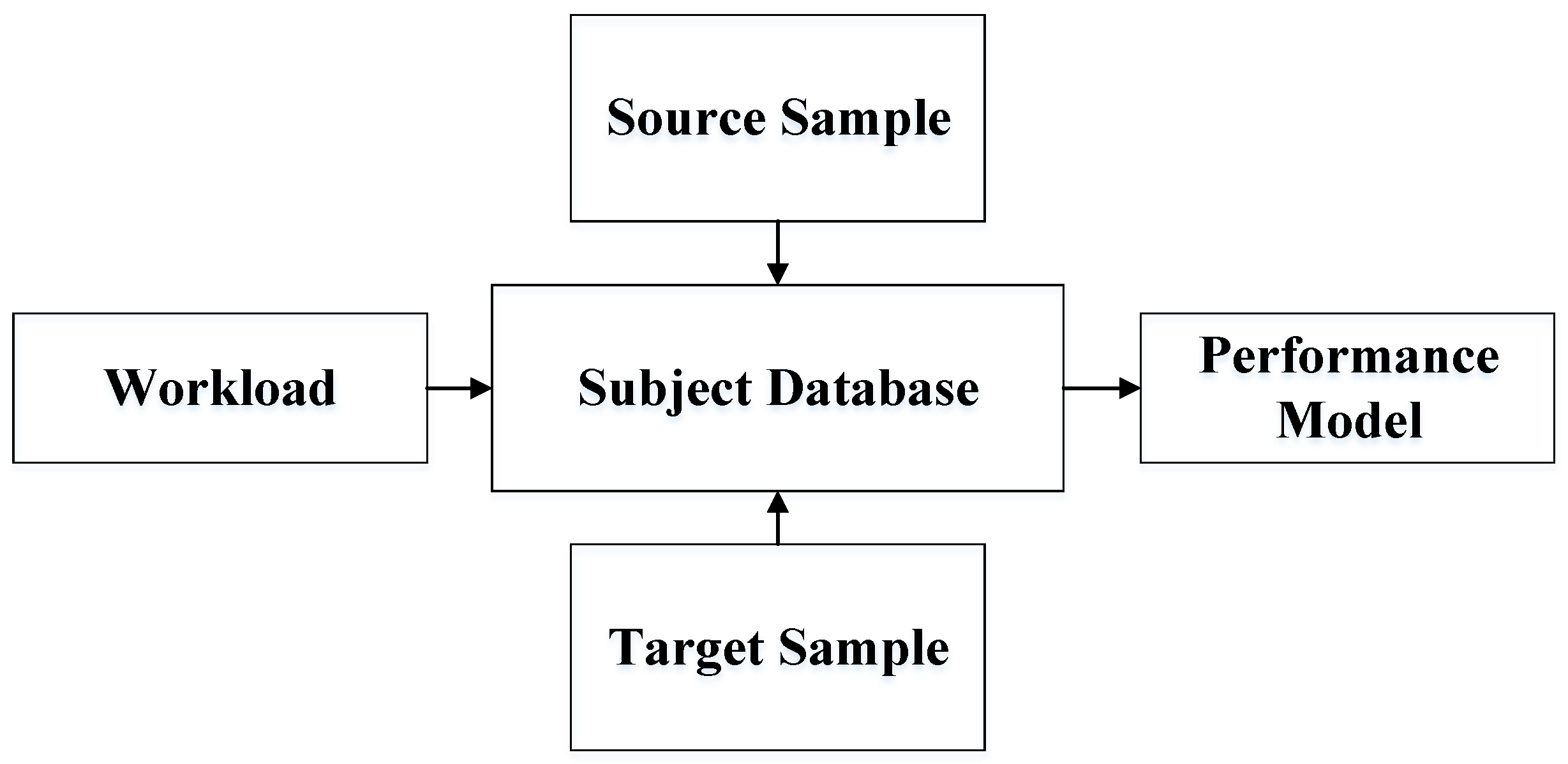
3.1. Problem Statement

In this paper, we focus on building an accurate performance model rapidly with a small amount of samples for a database system in a newer database version. For a given database and a specific workload, our object is to enable the reuse of previous performance measurements in an older database version to facilitate the performance prediction in a newer version. In order to formalize this problem concisely, we introduce some mathematical symbols to represent related concepts.
Configuration. A configuration of a database system is represented as a set x = ( c 1 , c 2 , , c n ) , where c i indicates the i-th configuration parameter of the database system and n is the number of configuration parameters. The configuration parameters can either be (1) an integer variable in the valid configuration bound of the parameter, (2) a categorical variable or a Boolean variable. The configuration space is a Cartesian product of all configuration parameters X = D o m ( c 1 ) × × D o m ( c n ) , where D o m ( c i ) is the valid range of each parameter.
Performance model. Performance (e.g., throughput or latency) is an essential non-functional property of database systems. Different configurations may lead to different performance values. We treat the performance as a black-box function, which describes how configuration parameters and their interactions influence the system performance. Given a database system A and a workload W with configuration space X , a performance model is a black-box function f : X R that maps each configuration x X of A to the performance of the system.
Sample. Due to the large configuration space and expensive measurement cost, researchers usually propose to measure the performance values of a limited number of configurations (called sample), then construct a performance model from these data to predict the performance values of any new configuration. We run a database A in a certain version v V on various configurations x i X , and record the resulting performance values y i . The training data for learning a performance model for system A with version v are D t r = ( x i , y i ) , i = 1 , 2 , , m , where m is the number of performance measurements. The database in an older version is called source domain, while the database in a newer version is called target domain. S S and S T indicate the samples in source and target, respectively.
The object is to learn a reliable performance model f ^ ( x ) in target domain. Specifically, we aim to minimize the prediction error over the configuration space:
arg min x X p e = | f ^ ( x ) f ( x ) | .
The difficulty of this problem is to use only a small sample while still be able to predict the performance of other unseen configurations with a high accuracy. In this paper, we import the measurements in source domain to help constructing a reliable performance prediction model in target domain. Thus, the inputs to this problem are a large number of samples from the source and a small number of samples from the target, while the output is a reliable performance model in target, as described in Figure 1.

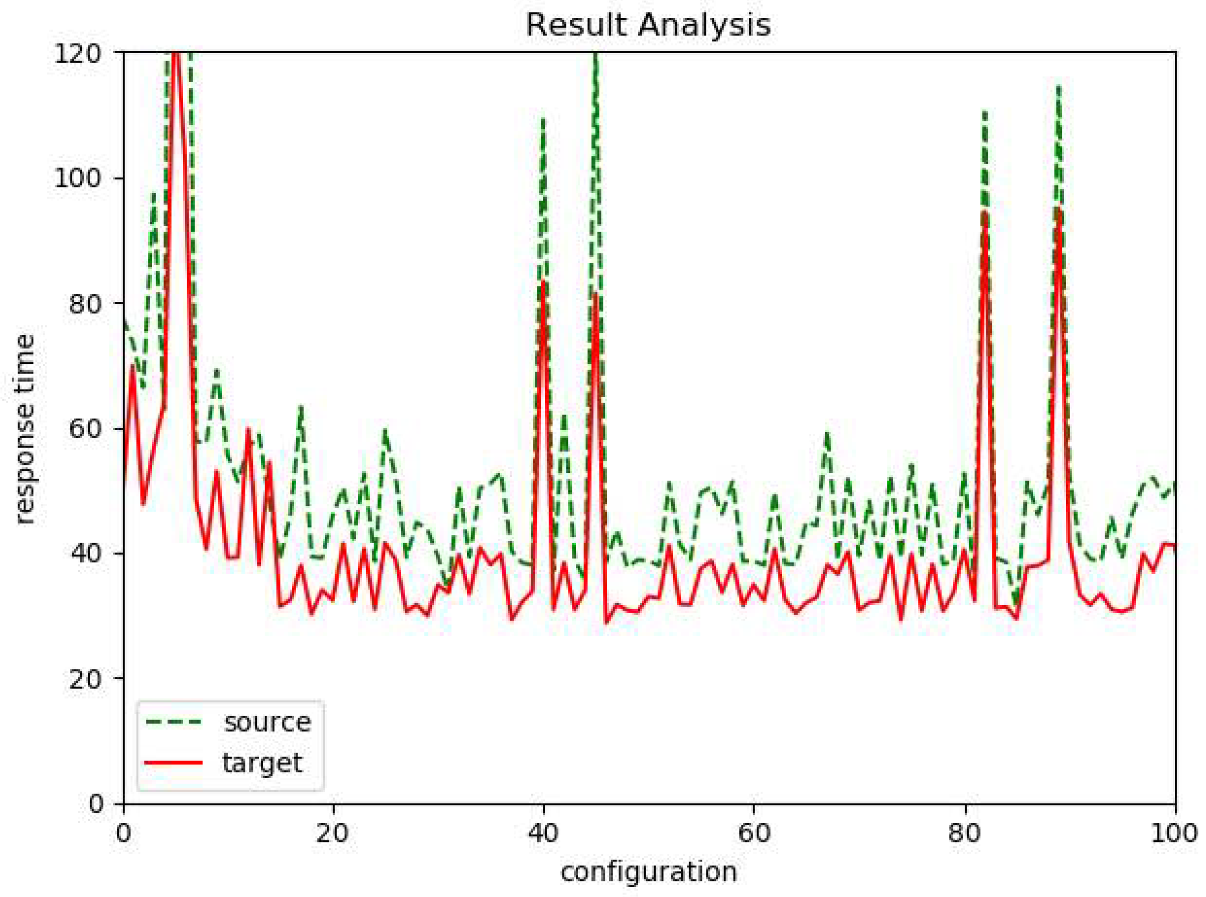
3.2. Key Observations

Generally, performance values are expected to differ in different database versions for a given configuration. Fortunately, performance models typically exhibit similarities across different database versions in the configuration space. An experiment is carried out to verify this observation, and the results are shown in Figure 2. We randomly select 100 valid configurations in MySQL, and obtain the performance measurements in both 5.5 and 8.0 versions, which are indicated by source and target, respectively. On the bases of the experimental results and some previous researches [17,34], we accept that the performance responses in source domain and target domain are similar in configuration space when database version changes.
The second key observation is that the performance response of a database system is reasonably smooth within a certain range, and it changes dramatically when some key parameters change. Intuitively, we expect that for nearby input points x 1 and x 2 in the smooth range, their corresponding output points y 1 and y 2 to be near-by as well. However, on the contrary, the performance responses of different regions vary greatly. The similar observations have been found in former studies [2,8].

3.3. Assumptions and Limitations

In reality, the correlations are quite strong in some version change situations, while for others, the correlations are extremely weak or even nonexistent. We assume that the strength of the correlation is related to the details of upgrades between versions. In some version update cases, the optimization features that are determined by the configuration options may undergo a substantial revision between different versions because algorithmic changes may significantly improve the way how the optimization features work. Nonetheless, some version updates do not influence the internal logic controlled by configuration parameters, thus the correlation remain strong in these cases. We focus on the latter case because that is the majority in database version update cases.
In addition, the number of configuration parameters changes as the database version updates. Some parameters are added and some are forbidden in the upgraded database version. We currently focus on the unchanged parameter from version to version for simplicity, and defer the problem of taking parameter change into consideration when transferring knowledge across different database versions as future work.

4. Partitioned Co-Kriging Based Performance Prediction
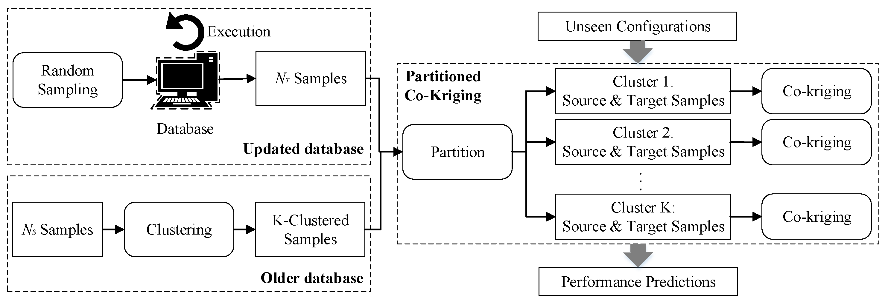
4.1. Overview

Our goal is to construct an accurate performance prediction model using a small sample in target domain. To overcome the challenge of insufficient sample, we reuse prior information that we can get from source domain to learn a performance model more efficiently. The foundation of our method is that performance responses in source and target have high correlations. Thus, the large samples in source can be applied to build a performance model in target. The performance prediction is realized by the co-kriging method.
The assumption of co-kriging method is that the performance response is stationary. In practice, the performance response of database is not stationary in the entire configuration space, but it is relatively smooth in different regions. Based on this characteristic, we propose to learn performance prediction models within each region. Therefore, we first need to solve the partition problem: how to divide the entire configuration space into several smooth regions?
Generally, there are only sparse samples in target due to the high cost in collecting the samples. The small samples provide too little information to perform the partitioning task. In contrast, the sample in source is usually readily available. As a consequence, we use the concept of relatedness between source and target to address the problem. The partition of configuration space can be achieved by clustering with the adequate samples from source domain. The prediction accuracy can be improved effectively by using this partition scheme.
Figure 3 illustrates the performance prediction process for unseen configurations in target. The input of PCK method incorporates performance measurements from both source and target. We use random sampling method to generate a small number of samples in target, while a large number of samples are available in source. According to the database performance characteristics, we consider dividing the entire configuration space into several smooth regions by clustering the sufficient performance measurements in source. With the region information of source samples, each target sample can determines its region by Euclidean distance. A target sample adopt the region information of a source sample which has the nearest Euclidean distance with it. Subsequently, we can learn corresponding performance models in different regions using all the samples and the partition information in configuration space. Finally, we can estimate the performance value for any unseen configuration with this performance prediction model.
In summary, we propose an innovative way of fast performance modeling in updated databases (newer database versions) using co-kriging. It makes use of the large number of source samples in two ways: (1) the abundant and easily accessible source samples can be reused to facilitate the construction of an accurate performance model, and (2) they can further provide partition information about the smooth region in configuration space due to the correlation of source and target, thus improve the prediction accuracy of the co-kriging-based prediction model.

4.2. Performance Prediction with Partitioned Co-Kriging

Using the above-mentioned prediction process, we now discuss the PCK method in Algorithm 1.
Random sampling. We collect training data in target domain by running a subject database with updated version on various configurations and record the resulting performance values. The selected configurations are generated by random sampling (RS) strategy, as it can effectively search for a large configuration space, especially when configuration parameters are not equally important [37] (line 1).
Clustering. The partition of configuration space is achieved by clustering the adequate source samples (line 2). We use a well-studied technique, called k-means [38], to cluster the source samples into meaningful groups. The goal of the k-means algorithm is to divide M points in N dimensions into K clusters so that the within-cluster sum of squares is minimized. M is the number of the source samples. N equals to the number of configuration parameters add one; it means that we consider not only each configuration parameter, but also its performance value in clustering. This is because we aim to identify the different smooth regions. K clusters correspond to K different regions.
Algorithm 1  P C K ( A , W , P , C B , S S , K , V M , C U ) .
Input: A: the subject database; W: workload; P: configuration parameters; C B : configuration bounds; S S : the available samples in source domain; K: the number of clusters; V M : variogram model; C U : the unseen configurations in target domain.
Output:  P U : performance predictions of the unseen configurations in target domain.
1:  S T R S ( N T , A , W , P , C B ) ;
2: K-clustered S S k m e a n s ( S S , K ) ;
3: K-clustered S T p a r t i t i o n ( S T , K-clustered S S );
4: K-clustered C U p a r t i t i o n ( C U , K-clustered S S );
5: for each c i C U  do
6:      p i c o k r i g i n g ( S S , S T , c i , V M ) in corresponding cluster;
7: end for
8: return  P U ;
One of the drawbacks of using k-means is that we have to specify the number of clusters (K) before starting. On the one hand, the accuracy of prediction models can be increased by clustering different smooth regions. On the other hand, K should not be selected too large because of the small sample in target. Otherwise, the sample size in each region will be too small to learn a reliable prediction model. In conclusion, choosing K is a trade-off, and we are going to explore this problem in our experiments.
Partition. After the clustering is complete, we get K smooth regions in configuration space. Then, K performance prediction models can be constructed using co-kriging. The input of co-kriging includes not only the source samples in the cluster, but also the target samples in corresponding region. In target domain, the region of a sample is determined by the Euclidean distances with source samples. In order to facilitate the co-kriging-based performance prediction in next step, the samples in both source and target are partitioned using the clustering results (line 3–4).
Co-kriging. Kriging, a regression method, is a minimum variance unbiased linear estimator and has received wide use for ore reserve estimation applications in mining [20]. Kriging utilizes the spatial correlation, of the variable of interest with itself, to determine the weights in an optimal manner. Co-kriging is the logical extension of ordinary kriging to situations where two or more variables are spatially interdependent and the one whose values are to be estimated is not sampled as intensively as the others with which it is correlated [19]. Its advantage is that when the primary variable is difficult or expensive to obtain, the co-kriging method adopts the auxiliary variable that is easier to obtain and is correlated with the primary variable to predict the primary variable, thus improving the prediction accuracy (line 6).
When the auxiliary variable is readily available and changes smoothly, such variable can be introduced into the co-kriging method as an auxiliary influencing factor. In this work, we employ co-kriging method to predict the performance of new configuration in an updated database version (target). Introducing the performance response in an older database version (source) as an auxiliary variable is conducive to the prediction result. In the application of co-kriging, a first step is to model the variogram for each variable as well as a cross-variogram for the two variables. Under the second-order stationary hypothesis, its expectation is
E [ Z 2 ( x ) ] = m 2 .
The cross-variogram is
γ 12 ( h ) = E [ Z 1 ( x + h ) Z 1 ( x ) ] [ Z 2 ( x + h ) Z 2 ( x ) ] .
Thus, the interpolation formula of co-kriging method is
Z 2 * ( x 0 ) = i = 1 N 1 λ 1 i Z 1 ( x 1 i ) + j = 1 N 2 λ 2 j Z 2 ( x 2 j ) .
where Z 2 * ( x 0 ) is the performance prediction value of configuration x 0 in target; Z 2 ( x 2 j ) indicates the performance measurement of each configuration in target; λ 2 j is the weight coefficient for performance measurement of each configuration in target; Z 1 ( x 1 i ) is the performance measurement of each configuration in source; λ 1 i is the weight coefficient for performance measurement of each configuration in source; N 1 , N 2 refer to the sample size of source and target, respectively; and N 1 > N 2 .
Two Lagrange multipliers u 1 and u 2 are introduced for derivation:
i = 1 N 1 λ 1 i γ 11 ( x 1 i x I ) + j = 1 N 2 λ 2 j γ 21 ( x 2 j x I ) + u 1 = γ 21 ( x 0 x I ) , i = 1 N 1 λ 1 i γ 21 ( x 1 i x J ) + j = 1 N 2 λ 2 j γ 22 ( x 2 j x J ) + u 2 = γ 22 ( x 0 x J ) , i = 1 , 2 , , N 1 , j = 1 , 2 , , N 2 , i = 1 N 1 λ 1 i = 0 , j = 1 N 2 λ 2 j = 1 .
where γ 11 and γ 22 are the variograms of Z 1 and Z 2 , separately. γ 12 and γ 21 are the cross-variograms for the two variables, and γ 12 = γ 21 .
By solving linear Equation (5), the weight coefficients ( λ 1 i , i = 1 , 2 , , N 1 ; λ 2 j , j = 1 , 2 , , N 2 ) and two Lagrange multipliers u 1 and u 2 can be obtained. Thus, the performance estimation of any configuration in the configuration space can be acquired from Equation (4).
Performance prediction. Given any unseen configuration in target, we first identify the region where it belongs according to the clustering results. The performance of the configuration is then predicted by co-kriging method using the samples and variogram model in this region, as described in Algorithm 1 (lines 5–8).

5. Experimental Evaluation

We have implemented the PCK and other algorithms, and conducted extensive experiments in diverse databases. The source code and the data can be found in the online repository: https://github.com/xdbdilab/PCK. In this section, we first describe our experiment setup, and then present the experimental results to prove the efficiency and effectiveness of the proposed approach.

5.1. Experimental Settings

Subject databases, versions, and benchmarks. We carried out an investigation into the subject systems of researches on configuration tuning for database systems [2,6,7,8,9,10,14,16,28,29,31,39,40,41,42,43,44], and chose five widely used database systems to evaluate PCK approach: MySQL (https://www.mysql.com/ (accessed on 25 September 2020)), PostgreSQL (https://www.postgresql.org/ (accessed on 26 September 2021)),SQLite (https://www.sqlite.org/ (accessed on 26 September 2021)), Redis (https://redis.io/ (accessed on 11 October 2020)), and Cassandra (http://cassandra.apache.org/ (accessed on 13 October 2020)). MySQL is an open-source relational database management system (RDBMS). PostgreSQL is an open-source object-relational database management system (ORDBMS). SQLite is an open-source embedded RDBMS. Redis is an open-source in-memory data structure store. Cassandra is an open-source column-oriented NoSQL database management system. In this experiment, we choose two (PostgreSQL, SQLite, and Cassandra) or three (MySQL, Redis) representative versions for convenience. The time gaps among these releases of three database are about five years for PostgreSQL, nearly a half year for SQLite, about five and a half years for Cassandra, and approximate three years for MySQL and Redis. In addition, we use sysbench (https://github.com/akopytov/sysbench (accessed on 25 September 2020)) for MySQL, pgbench (https://www.postgresql.org/docs/11/pgbench.html (accessed on 26 September 2021)) for PostgreSQL, a customized workload for SQLite, YCSB [45] for Cassandra, and Redis-Bench (https://redis.io/topics/benchmarks (accessed on 11 October 2020)) for Redis.
Parameters. For each database system, we use domain expertise to identify a subset of parameters that are considered critical to the performance, as in [2,9,10]. Reducing the number of considered parameters can reduce the search space exponentially, and numerous existing approaches [9,12] also adopt this manual feature selection strategy. Note that even with only these parameters, the search space is still enormous, and exhaustive search is infeasible. Table 1 summarizes the database systems and versions, along with the benchmarks, the numbers of selected parameters, and performance metrics, respectively.
Running environment. In order to avoid interference in collecting samples from different subject database systems, we conduct experiments on different servers and computer. In addition, we ensure a consistent running environment for different versions of the same subject system. The running environments for different subject databases systems are listed as follows.
MySQL, PostgreSQL: The physical server is equipped with two 2-core Intel(R) Core(TM) i5-4590 CPU @3.30GHZ processors, 4GB RAM, 64GB disk, and running CentOS 6.5 and Java 1.8.0.
SQLite: The computer is equipped with a Intel(R) Core(TM) i5-4460 CPU @3.20GHZ processors, 8GB RAM, 1TB disk, and running Windows 10 and Java 1.8.0_291.
Redis: The cloud server is equipped with two 2-core Intel(R) Xeon(R) Platinum 8163 CPU @2.50GHz processors, 4GB RAM, 53.7GB disk, and running CentOS 7.6 and Java 1.8.0_261.
Cassandra: The physical server is equipped with two 4-core Intel(R) Xeon(R) CPU E5-2683 V3 @2.00GHz processors, 32GB RAM, 86GB disk, and running CentOS 6.5 and Java 1.8.0_211.
Baseline Algorithms. To evaluate the performance of PCK approach, we compare it with six state-of-the-art algorithms: DeepPerf [10], CART [3], Finetune [46], DDC [47], Model-shift [33], and Ottertune [2]. We provide a brief description for each algorithm as follows.
DeepPerf and CART establish performance prediction models in target domain directly. They consider the performance prediction problem as a nonlinear regression problem and apply different machine learning methods, namely Deep Neural Network (DNN) and the Classification and Regression Trees (CART) technique, to find this nonlinear model.
Finetune and DDC are two widely used transfer learning schemes. Finetune is a network-based transfer learning method. It freezes the partial network that pre-trained in the source domain, and transfers it to be a part of DNN which used in target domain. DDC is a mapping-based transfer learning, which maps instances from the source and target into a new data space.
Model-shift approach shifts the model that has been learned in the source to predict the system performance in the target using linear regression models. CART is applied to build performance prediction models in source domain.
Ottertune is a transfer learning approach that exploits source samples to learn a performance model in the target. The Gaussian Process (GP) model is used to learn a performance model that can predict unobserved response values.

5.2. Evaluation of Prediction Accuracy

Data collection. We use the random sampling strategy to generate a set of configurations for each database and test them on the database system with given workloads on different versions to get the performance measurements. A configuration–performance pair is regarded as a sample. The numbers of samples for MySQL, PostgreSQL, SQLite, Redis, and Cassandra are 294, 300, 280, 323, and 1129, respectively. The collection of all source samples serves as auxiliary training data. In the target domain, a subset of these samples is selected randomly for training dataset; the remaining samples serve as the testing dataset.
Evaluation metric. Holdout validation is employed to compare the prediction accuracy between different methods. We use the training dataset and auxiliary training data to generate a performance model for each method, and then use this model to predict performance values of configurations in the testing dataset. We select Mean Relative Error (MRE) as a metric for evaluating prediction accuracy, which is computed as follows:
M R E = 1 N i = 1 N | a i p i | a i × 100
where N is a total number of configurations in the testing dataset, and a i and p i represent the actual performance value and predicted performance value, respectively. We choose this metric as it is widely used to measure the accuracy of prediction models [5,10,33,34].
Performance results. We run PCK method and six baseline algorithms for five subject database systems independently. The size of training dataset in target domain is set to c × n , where c is the number of selected configuration parameters for each subject database system (which is shown in the column # of selected parameters of Table 1), and n ranges from 1 to 15. To evaluate the consistency and stability of the approaches, for each sample size of each subject database system, we repeat the random sampling, training and testing process 5 times. We then show and compare the mean of the MREs obtained with the 7 different approaches for each sample size. The experiment results of five subject database systems for larger version changes are listed in Table 2, Table 3, Table 4, Table 5 and Table 6, respectively.
As expected, our proposed method has achieved better performance than all other six algorithms. Specifically, for five subject database systems, PCK outperforms all other six baseline algorithms: 24.99–53.18% improvement over DeepPerf, 14.20–51.19% improvement over CART, 4.42–46.58% improvement over Finetune, 25.26–53.13% improvement over DDC, 9.34–50.03% improvement over Model-shift, and 46.80–69.42% over Ottertune. The improvement percentages are shown in Figure 4. For the sake of simplicity, the data in Figure 4 is obtained by averaging the MRE data of different sample sizes in each subject database system.
DeepPerf tackles the performance prediction problem directly by training a performance model with DNN. Further, Finetune and DDC are two DNN-based transfer learning approaches. The above experimental results show that the MRE results of PCK are better than these three DNN-based performance modeling methods. It is because that training a high-performance DNN often requires a large amount of training data, but we can only provide a small sample due to the high cost of performance measurement.
In another aspect, we find out that the two DNN-based transfer learning methods in most cases perform higher prediction accuracy than simple DNN-based performance prediction model in five database systems. Similarly, the Model-shift approach transfers the CART-based performance model in the source to the target using linear regression models, and it also achieves better MRE than CART. This observation verifies the effectiveness of transfer learning on performance prediction task.
The validity of above-mentioned transfer learning methods proves that there exists a correlation between the source and target. Our proposed PCK method aims to take advantage of this correlation to build a high-performance prediction model in target domain. In the experiment results, the PCK achieves higher prediction accuracy compared with other four transfer learning method under almost all the sample sizes.
From another point of view, PCK requires a much smaller number of target samples to reach the same standard of prediction accuracy, compared with other baseline approaches. It means that PCK outperforms six baseline algorithms not only in terms of prediction accuracy, but also in terms of measurement effort.
To further verify our conclusion, we conduct the similar experiments across different version changes. The MRE comparison among different approaches for MySQL and Redis under different version change scenarios (version 5.5–5.7, 5.7–8.0 for MySQL, and version 4.0.1–5.0.0, 5.0.0–6.0.5 for Redis) are listed in Table 7, Table 8, Table 9 and Table 10, respectively. Experimental results confirm that the PCK outperforms the state-of-the-art baselines in terms of prediction accuracy and measurement cost in almost all experimental settings in this paper.

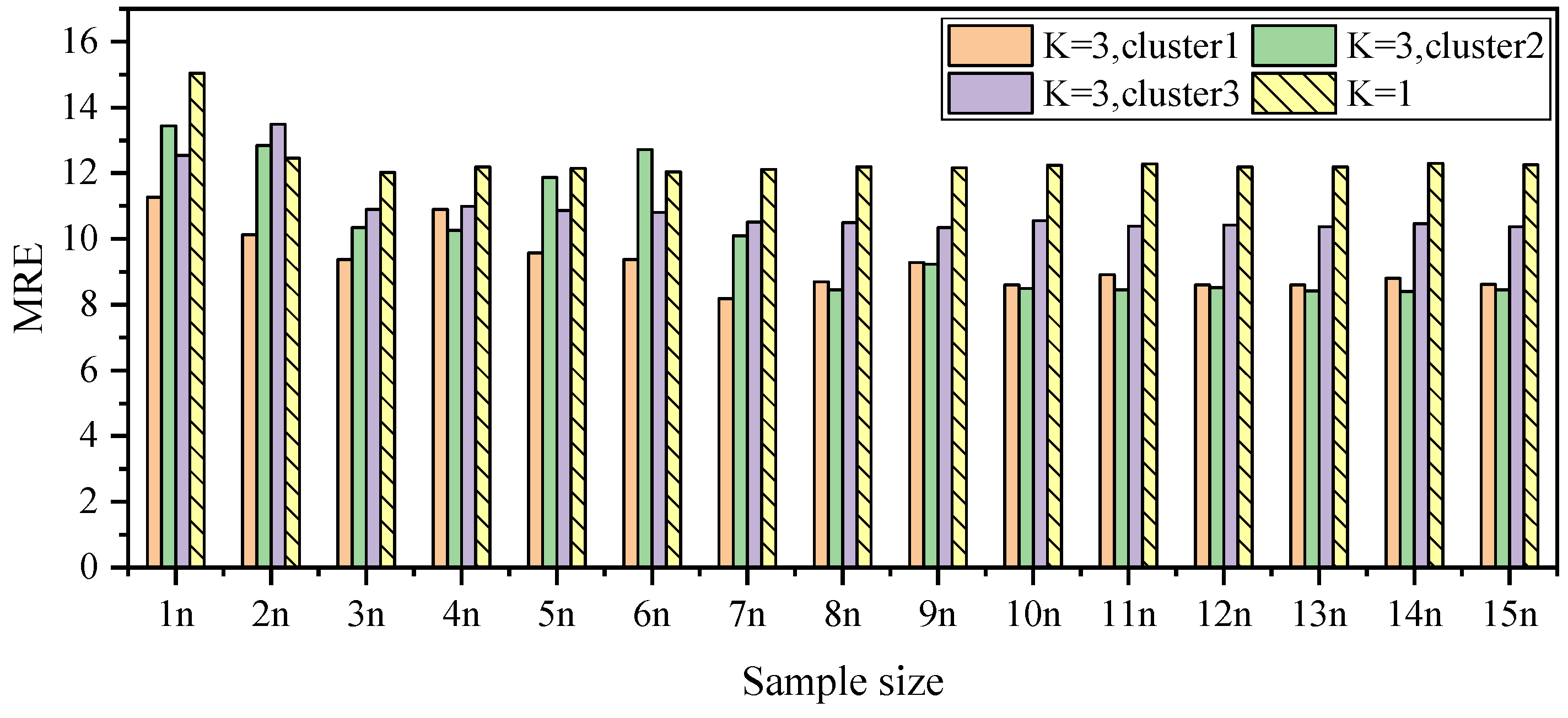
5.3. Trade-Off on Choosing K

In this part, we will discuss the trade-off on choosing the number of clusters (K), and illustrate the influence of different K values on the prediction accuracy. In order to explore this problem, we systematically vary the value of K from 1 to 10 in each subject system and we measure the prediction accuracy in each case. Taking MySQL (version 5.5–8.0) as an example, the experiment results are shown in Table 11.
Our results, in Table 11, indicate that PCK achieves the highest prediction accuracy for almost all sample sizes when K equals to 3 in MySQL. The MRE of PCK decreases when K increases appropriately. This demonstrates that clustering different smooth regions could help boost the performance of prediction model. However, the prediction accuracy will not continue to grow when K exceeds a certain threshold, such as 3 in the above example. This is due to the insufficient target samples. If a large K is chosen in PCK, the available target sample in each region will be too little to learn a reliable performance model. Consequently, the choice of K is the key to whether the PCK method can achieve high prediction accuracy.
In order to further verify the necessity of PCK, we compare the MRE in different clusters ( K = 3 ) with the MRE without clustering ( K = 1 ) in MySQL, the result is shown in Figure 5. We observe that the MRE without clustering is higher than the MRE in three different clusters in almost all sample sizes. Finally, the optimal prediction accuracy is achieved in this case ( K = 3 ). In addition, PCK achieves the best prediction performance in Redis (version 4.0.1–6.0.5) and PostgreSQL (version 9.3–11.0) when K = 2 , and K = 1 in Cassandra (version 2.1.0–3.11.6), K = 4 in SQLite (version 3.31.1–3.36.0), respectively. The reason for the small K in Cassandra is its larger configuration space, thus the insufficient measurements may lead to inaccurate partitioning.

6. Discussion

6.1. Prediction Accuracy

Experimental results on five different database systems are shown in Table 2, Table 3, Table 4, Table 5 and Table 6, respectively. Our PCK method achieved better prediction accuracy than all the baseline algorithms. The MRE reduction of PCK over six state-of-the-art baseline algorithms rages from 30.73% to 60.83% on average. The reason for this result is that PCK can leverage the transferable knowledge in source to facilitate the performance modeling in target. The existence of transferable knowledge is based on the strong correlation between the performance responses of different versions.
We conducted experiments in different version change scenarios of the same subject database system, and the results confirmed this fact. The MRE comparisons of PCK among different version change scenarios for MySQL (as shown in Table 2, Table 7, and Table 8) and Redis (as shown in Table 5, Table 9, and Table 10) indicate that the smaller the version changes, the higher the prediction accuracy achieved by PCK. This result is intuitive because the smaller version change often means a stronger correlation between source and target.
In addition, an appropriate value of K can guarantee the high prediction accuracy achieved by PCK, as demonstrated in Table 11. The trade-off of choosing the value of K mainly lies in the tradeoff between the precise partition of configuration space and the insufficient samples in target. The optimal K is usually small because of the limited samples in target, thus it can be obtained simply through a few experiments.

6.2. Measurement Effort

In this paper, we assume that a number of available performance measurements in the source are available, while in the target there is a lack of samples. This is reasonable because the source database has been running for a relative long time and has been deeply studied by database administrators. Thus, we can obtain sufficient samples at a low cost and avoid the overhead of collecting a large number of samples in source. Therefore, the measurement effort in this paper refers specifically to performance measurements in the target. Experimental results on five different database systems show that PCK can achieve better performance prediction accuracy with less samples in target. To reach the same standard of prediction accuracy, almost all the baseline algorithms require more than 15 times of performance measurements in target compared with our PCK method. These results suggest that PCK can effectively decrease the measurement cost in performance prediction tasks across different database versions.

6.3. Effectiveness of Transfer Learning

We select DeepPerf and CART as baselines to verify the effectiveness of transfer learning. These two approaches establish performance prediction models in target domain directly. We also evaluate the performance of transfer learning schemes based on DeepPerf and CART given the measurements of source database. Finetune and DDC are two widely used transfer learning schemes, and we use these two schemes on the basis of DeepPerf in this paper. Similarly, Model-shift approach uses linear regression models to shift the CART model that has been learned in the source to predict the performance of the system in the target.
Experimental results confirm the effectiveness of transfer learning. Among all the experimental settings (namely different database systems, different version change scenarios, and different sample sizes) in this paper, the probabilities that the transfer learning-based approaches perform better than the directly learning approaches are 99.3% for Finetune, 61.5% for DDC, and 74.8% for Model-shift, respectively. In other words, Finetune and DDC perform higher prediction accuracy than DeepPerf, meanwhile, Model-shift approach obtains better predication performance than CART under most conditions. Therefore, utilizing the transferable knowledge across environments is a promising direction to contribute to learning faster, better, and less costly performance models.

7. Conclusions and Future Work

The current approaches target a specific database version where one needs to learn a performance model from scratch for a newer database version. In this paper, we target the use case when the database version updates. We proposed PCK, a fast performance modeling strategy, which is orthogonal to the previously proposed modeling method. By exploiting knowledge pieces from source via both clustering and co-kriging, our proposed PCK approach significantly improves prediction accuracy and reduces excessive measurement effort of performance modeling. Experimental results on five different database systems show that PCK can achieve better performance prediction accuracy with fewer data in target. The MRE reduction of PCK over six state-of-the-art baseline algorithms rages from 30.73% to 60.83% on average. To achieve the same prediction accuracy, PCK can save more than 15 times of measurements in target compared with other approaches. Furthermore, the experimental results verify the effectiveness of transfer learning on performance prediction task.
Currently, PCK is suitable for the version change scenarios that the correlation of performance responses remains strong. It is possible to introduce a scheme to identify whether the correlation is strong or weak after the database version changes, and this will be one of our future work. Besides, our proposed method focuses on the unchanged parameter in source and target. In the future, we will continue to improve the PCK to take parameter changes (added and forbidden parameters) into consideration when transferring knowledge across different database versions. Note that PCK is proposed for the database version change scenarios. However, there are varying use cases, namely different kinds of environmental changes, such as workload change and hardware change scenarios. We will explore the usability of PCK and its variants in other environmental change scenarios, this is also an interesting future issue.

Author Contributions

Conceptualization, L.B. and R.C.; methodology, L.B. and R.C.; software, S.W. and J.D.; validation, S.W., X.W., Y.D. and R.S.; formal analysis, R.C., L.B. and S.W.; investigation, S.W., X.W., Y.D. and R.S.; resources, L.B.; data curation, S.W., X.W., Y.D. and R.S.; writing—original draft preparation, R.C.; writing—review and editing, L.B. and J.D.; visualization, R.C. and J.D.; supervision, L.B.; project administration, R.C. and X.W.; funding acquisition, L.B. All authors have read and agreed to the published version of the manuscript.

Funding

This research was funded in part by the National Key R&D Program of China under Grant No. 2018YFC0831200, in part by National Natural Science Foundation of China under Grant No. 61202040 with Xidian University, in part by the Key R&D Program of Shaanxi under Grant No. 2019ZDLGY13-03-02, in part by Natural Science Foundation of Shaanxi Province, China under Grant No. 2019JM-368, and in part by the Key R&D Program of Hebei under Grant No. 20310102D.

Institutional Review Board Statement

Not applicable.

Informed Consent Statement

Not applicable.

Data Availability Statement

Data available in a publicly accessible repository that does not issue DOIs. Publicly available datasets were analyzed in this study. This data can be found here: https://github.com/xdbdilab/PCK.

Conflicts of Interest

The authors declare no conflict of interest.

References

  1. Xu, T.; Jin, L.; Fan, X.; Zhou, Y.; Pasupathy, S.; Talwadker, R. Hey, You Have given Me Too Many Knobs!: Understanding and Dealing with over-Designed Configuration in System Software. In Proceedings of the 2015 10th Joint Meeting on Foundations of Software Engineering, Bergamo, Italy, 30 August 2015–4 September 2015; pp. 307–319. [Google Scholar]
  2. Van Aken, D.; Pavlo, A.; Gordon, G.J.; Zhang, B. Automatic database management system tuning through large-scale machine learning. In Proceedings of the 2017 ACM International Conference on Management of Data, Chicago, IL, USA, 14–19 May 2017; pp. 1009–1024. [Google Scholar]
  3. Guo, J.; Czarnecki, K.; Apel, S.; Siegmund, N.; Wąsowski, A. Variability-aware performance prediction: A statistical learning approach. In Proceedings of the 2013 28th IEEE/ACM International Conference on Automated Software Engineering (ASE), Silicon Valley, CA, USA, 11–15 November 2013; pp. 301–311. [Google Scholar]
  4. Lu, J.; Chen, Y.; Herodotou, H.; Babu, S. Speedup your analytics: Automatic parameter tuning for databases and big data systems. Proc. VLDB Endow. 2019, 12, 1970–1973. [Google Scholar] [CrossRef] [Green Version]
  5. Guo, J.; Yang, D.; Siegmund, N.; Apel, S.; Sarkar, A.; Valov, P.; Czarnecki, K.; Wasowski, A.; Yu, H. Data-efficient performance learning for configurable systems. Empir. Softw. Eng. 2018, 23, 1826–1867. [Google Scholar] [CrossRef] [Green Version]
  6. Duan, S.; Thummala, V.; Babu, S. Tuning database configuration parameters with iTuned. Proc. VLDB Endow. 2009, 2, 1246–1257. [Google Scholar] [CrossRef] [Green Version]
  7. Mahgoub, A.; Wood, P.; Ganesh, S.; Mitra, S.; Gerlach, W.; Harrison, T.; Meyer, F.; Grama, A.; Bagchi, S.; Chaterji, S. Rafiki: A middleware for parameter tuning of nosql datastores for dynamic metagenomics workloads. In Proceedings of the 18th ACM/IFIP/USENIX Middleware Conference, Las Vegas, NV, USA, 11–15 December 2017; pp. 28–40. [Google Scholar]
  8. Bao, L.; Liu, X.; Wang, F.; Fang, B. ACTGAN: Automatic Configuration Tuning for Software Systems with Generative Adversarial Networks. In Proceedings of the 2019 34th IEEE/ACM International Conference on Automated Software Engineering (ASE), San Diego, CA, USA, 11–15 November 2019; pp. 465–476. [Google Scholar]
  9. Zhu, Y.; Liu, J.; Guo, M.; Bao, Y.; Ma, W.; Liu, Z.; Song, K.; Yang, Y. Bestconfig: Tapping the performance potential of systems via automatic configuration tuning. In Proceedings of the 2017 Symposium on Cloud Computing, Santa Clara, CA, USA, 24–27 September 2017; pp. 338–350. [Google Scholar]
  10. Ha, H.; Zhang, H. Deepperf: Performance prediction for configurable software with deep sparse neural network. In Proceedings of the 2019 IEEE/ACM 41st International Conference on Software Engineering (ICSE), Montreal, QC, Canada, 25–31 May 2019; pp. 1095–1106. [Google Scholar]
  11. Nair, V.; Menzies, T.; Siegmund, N.; Apel, S. Faster discovery of faster system configurations with spectral learning. Autom. Softw. Eng. 2018, 25, 247–277. [Google Scholar] [CrossRef]
  12. Sarkar, A.; Guo, J.; Siegmund, N.; Apel, S.; Czarnecki, K. Cost-efficient sampling for performance prediction of configurable systems (t). In Proceedings of the 2015 30th IEEE/ACM International Conference on Automated Software Engineering (ASE), Lincoln, NE, USA, 9–13 November 2015; pp. 342–352. [Google Scholar]
  13. Valov, P.; Guo, J.; Czarnecki, K. Empirical comparison of regression methods for variability-aware performance prediction. In Proceedings of the 19th International Conference on Software Product Line, Nashville, TN, USA, 20–24 July 2015; pp. 186–190. [Google Scholar]
  14. Nair, V.; Menzies, T.; Siegmund, N.; Apel, S. Using bad learners to find good configurations. In Proceedings of the 2017 11th Joint Meeting on Foundations of Software Engineering, Paderborn, Germany, 4–8 September 2017; pp. 257–267. [Google Scholar]
  15. Jamshidi, P.; Velez, M.; Kästner, C.; Siegmund, N. Learning to sample: Exploiting similarities across environments to learn performance models for configurable systems. In Proceedings of the 2018 26th ACM Joint Meeting on European Software Engineering Conference and Symposium on the Foundations of Software Engineering, Lake Buena Vista, FL, USA, 4–9 November 2018; pp. 71–82. [Google Scholar]
  16. Zhang, J.; Liu, Y.; Zhou, K.; Li, G.; Xiao, Z.; Cheng, B.; Xing, J.; Wang, Y.; Cheng, T.; Liu, L.; et al. An end-to-end automatic cloud database tuning system using deep reinforcement learning. In Proceedings of the 2019 International Conference on Management of Data, Amsterdam, The Netherlands, 30 June 2019–5 July 2019; pp. 415–432. [Google Scholar]
  17. Jamshidi, P.; Siegmund, N.; Velez, M.; Kästner, C.; Patel, A.; Agarwal, Y. Transfer learning for performance modeling of configurable systems: An exploratory analysis. In Proceedings of the 2017 32nd IEEE/ACM International Conference on Automated Software Engineering (ASE), Urbana, IL, USA, 30 October–3 November 2017; pp. 497–508. [Google Scholar]
  18. Pan, S.J.; Yang, Q. A survey on transfer learning. IEEE Trans. Knowl. Data Eng. 2009, 22, 1345–1359. [Google Scholar] [CrossRef]
  19. Oliver, M.A.; Webster, R. Kriging: A method of interpolation for geographical information systems. Int. J. Geogr. Inf. Syst. 1990, 4, 313–332. [Google Scholar] [CrossRef]
  20. Myers, D.E. CO-KRIGING: Methods and alternatives. In The Role of Data in Scientific Progress; Glaeser, P.S., Ed.; Elsevier Science Publisher: North-Holland, The Netherlands, 1985; pp. 425–428. [Google Scholar]
  21. Zhang, Y.; Guo, J.; Blais, E.; Czarnecki, K. Performance prediction of configurable software systems by fourier learning (t). In Proceedings of the 2015 30th IEEE/ACM International Conference on Automated Software Engineering (ASE), Lincoln, NE, USA, 9–13 November 2015; pp. 365–373. [Google Scholar]
  22. Zhang, Y.; Guo, J.; Blais, E.; Czarnecki, K.; Yu, H. A mathematical model of performance-relevant feature interactions. In Proceedings of the 20th International Systems and Software Product Line Conference, Beijing, China, 16–23 September 2016; pp. 25–34. [Google Scholar]
  23. Kolesnikov, S.; Siegmund, N.; Kästner, C.; Grebhahn, A.; Apel, S. Tradeoffs in modeling performance of highly configurable software systems. Softw. Syst. Model. 2019, 18, 2265–2283. [Google Scholar] [CrossRef]
  24. Narayanan, D.; Thereska, E.; Ailamaki, A. Continuous resource monitoring for self-predicting DBMS. In Proceedings of the 13th IEEE International Symposium on Modeling, Analysis, and Simulation of Computer and Telecommunication Systems, Atlanta, GA, USA, 27–29 September 2005; pp. 239–248. [Google Scholar]
  25. Tran, D.N.; Huynh, P.C.; Tay, Y.C.; Tung, A.K. A new approach to dynamic self-tuning of database buffers. ACM Trans. Storage (TOS) 2008, 4, 1–25. [Google Scholar] [CrossRef]
  26. Tian, W.; Martin, P.; Powley, W. Techniques for automatically sizing multiple buffer pools in DB2. In Proceedings of the 2003 Conference of the Centre for Advanced Studies on Collaborative Research, Toronto, ON, Canada, 6–9 October 2003; pp. 294–302. [Google Scholar]
  27. Thummala, V.; Babu, S. iTuned: A tool for configuring and visualizing database parameters. In Proceedings of the 2010 ACM SIGMOD International Conference on Management of Data, Indianapolis, IN, USA, 6–10 June 2010; pp. 1231–1234. [Google Scholar]
  28. Tan, J.; Zhang, T.; Li, F.; Chen, J.; Zheng, Q.; Zhang, P.; Qiao, H.; Shi, Y.; Cao, W.; Zhang, R. ibtune: Individualized buffer tuning for large-scale cloud databases. Proc. VLDB Endow. 2019, 12, 1221–1234. [Google Scholar] [CrossRef] [Green Version]
  29. Li, G.; Zhou, X.; Li, S.; Gao, B. Qtune: A query-aware database tuning system with deep reinforcement learning. Proc. VLDB Endow. 2019, 12, 2118–2130. [Google Scholar] [CrossRef]
  30. Tan, Z.; Babu, S. Tempo: Robust and self-tuning resource management in multi-tenant parallel databases. Proc. VLDB Endow. 2016, 9, 720–731. [Google Scholar] [CrossRef] [Green Version]
  31. Mahgoub, A.; Wood, P.; Medoff, A.; Mitra, S.; Meyer, F.; Chaterji, S.; Bagchi, S. SOPHIA: Online reconfiguration of clustered nosql databases for time-varying workloads. In Proceedings of the 2019 USENIX Annual Technical Conference, Renton, WA, USA, 10–12 July 2019; pp. 223–240. [Google Scholar]
  32. Zhang, B.; Van Aken, D.; Wang, J.; Dai, T.; Jiang, S.; Lao, J.; Sheng, S.; Pavlo, A.; Gordon, G.J. A demonstration of the ottertune automatic database management system tuning service. Proc. VLDB Endow. 2018, 11, 1910–1913. [Google Scholar] [CrossRef] [Green Version]
  33. Valov, P.; Petkovich, J.C.; Guo, J.; Fischmeister, S.; Czarnecki, K. Transferring performance prediction models across different hardware platforms. In Proceedings of the 8th ACM/SPEC on International Conference on Performance Engineering, L’Aquila, Italy, 22–26 April 2017; pp. 39–50. [Google Scholar]
  34. Jamshidi, P.; Velez, M.; Kästner, C.; Siegmund, N.; Kawthekar, P. Transfer learning for improving model predictions in highly configurable software. In Proceedings of the 2017 IEEE/ACM 12th International Symposium on Software Engineering for Adaptive and Self-Managing Systems (SEAMS), Buenos Aires, Argentina, 22–23 May 2017; pp. 31–41. [Google Scholar]
  35. Javidian, M.A.; Jamshidi, P.; Valtorta, M. Transfer learning for performance modeling of configurable systems: A causal analysis. arXiv 2019, arXiv:1902.10119. [Google Scholar]
  36. Krishna, R.; Nair, V.; Jamshidi, P.; Menzies, T. Whence to Learn? Transferring Knowledge in Configurable Systems using BEETLE. IEEE Trans. Softw. Eng. 2020. [Google Scholar] [CrossRef] [Green Version]
  37. Bergstra, J.; Bengio, Y. Random Search for Hyper-Parameter Optimization. J. Mach. Learn. Res. 2012, 13, 281–305. [Google Scholar]
  38. Wong, J.A.H.A. Algorithm AS 136: A K-Means Clustering Algorithm. J. R. Stat. Soc. 1979, 28, 100–108. [Google Scholar]
  39. Siegmund, N.; Grebhahn, A.; Apel, S.; Kästner, C. Performance-influence models for highly configurable systems. In Proceedings of the 2015 10th Joint Meeting on Foundations of Software Engineering, Bergamo, Italy, 30 August–4 September2015; pp. 284–294. [Google Scholar]
  40. Ishihara, Y.; Shiba, M. Dynamic Configuration Tuning of Working Database Management Systems. In Proceedings of the 2020 IEEE 2nd Global Conference on Life Sciences and Technologies (LifeTech), Kyoto, Japan, 10–12 March 2020; pp. 393–397. [Google Scholar]
  41. Zheng, C.; Ding, Z.; Hu, J. Self-tuning performance of database systems with neural network. In International Conference on Intelligent Computing, Proceedings of the Intelligent Computing Theory, ICIC 2014, Taiyuan, China, 3–6 August 2014; Springer: Cham, Switzerland, 2014; pp. 1–12. [Google Scholar]
  42. Debnath, B.K.; Lilja, D.J.; Mokbel, M.F. SARD: A statistical approach for ranking database tuning parameters. In Proceedings of the 2008 IEEE 24th International Conference on Data Engineering Workshop, Cancun, Mexico, 7–12 April 2008; pp. 11–18. [Google Scholar]
  43. Kanellis, K.; Alagappan, R.; Venkataraman, S. Too many knobs to tune? towards faster database tuning by pre-selecting important knobs. In Proceedings of the 12th USENIX Workshop on Hot Topics in Storage and File Systems (HotStorage 20), Virtual, 13–14 July 2020. [Google Scholar]
  44. Mahgoub, A.; Medoff, A.M.; Kumar, R.; Mitra, S.; Klimovic, A.; Chaterji, S.; Bagchi, S. OPTIMUSCLOUD: Heterogeneous Configuration Optimization for Distributed Databases in the Cloud. In Proceedings of the 2020 USENIX Annual Technical Conference (USENIX ATC 20), Virtual, 15–17 July 2020; pp. 189–203. [Google Scholar]
  45. Cooper, B.F.; Silberstein, A.; Tam, E.; Ramakrishnan, R.; Sears, R. Benchmarking cloud serving systems with YCSB. In Proceedings of the 1st ACM Symposium on Cloud Computing, Indianapolis, IN, USA, 10–11 June 2010; pp. 143–154. [Google Scholar]
  46. Yosinski, J.; Clune, J.; Bengio, Y.; Lipson, H. How Transferable Are Features in Deep Neural Networks? In Proceedings of the 27th International Conference on Neural Information Processing Systems, Montreal, QC, Canada, 8–13 December 2014; MIT Press: Cambridge, MA, USA, 2014; Volume 2, pp. 3320–3328. [Google Scholar]
  47. Tzeng, E.; Hoffman, J.; Zhang, N.; Saenko, K.; Darrell, T. Deep domain confusion: Maximizing for domain invariance. arXiv 2014, arXiv:1412.3474. [Google Scholar]
Figure 1. Problem overview of performance modeling across different database versions.
Applsci 11 09669 g001
Figure 2. Performance models exhibit similarities across different database versions.
Applsci 11 09669 g002
Figure 3. Overview of partitioned co-kriging approach.
Applsci 11 09669 g003
Figure 4. MRE improvement of PCK compared with six baseline algorithms.
Applsci 11 09669 g004
Figure 5. MRE comparison in different cluster ( K = 3 ).
Applsci 11 09669 g005
Table 1. Subject databases and versions, benchmarks, parameters, and performance metrics.
Subject DatabaseCategorySubject VersionsBenchmark# of Selected ParametersPerformance
MySQLRDBMS5.5, 5.7, 8.0sysbench10Latency (ms)
PostgreSQLORDBMS9.3, 11.0pgbench9Transactions per second
SQLiteEmbedded DB3.31.1, 3.36.0Customized8Transactions per second
RedisIn-memory DB4.0.1, 5.0.0, 6.0.5Redis-Bench9Requests per second
CassandraNoSQL DB2.1.0, 3.11.6YCSB28Throughput (MB/s)
Table 2. MRE comparison among different approaches for MySQL (version 5.5–8.0).
Sample Size1n2n3n4n5n6n7n8n9n10n11n12n13n14n15n
DeepPerf21.82924.65321.44622.75723.05023.23421.50821.31320.84921.03315.44419.55816.97016.49317.168
CART23.28122.51116.52919.26818.07113.55013.89912.64212.08613.03512.65111.1449.66512.93710.359
Finetune14.53213.85413.32012.64012.64913.37613.61014.90614.46712.52714.55013.70314.05014.03713.087
DDC19.25525.56326.35021.32521.91222.09624.01718.91719.93619.17419.28519.93517.63215.66116.233
Model-shift15.84816.17111.31411.24812.90210.12811.34210.22410.69711.06411.41910.82210.21711.19811.246
Ottertune16.84619.04118.60521.73719.47519.25819.29318.32219.08118.94517.39319.10017.99117.37916.504
PCK12.39912.17710.22210.73410.74710.9229.6189.2689.6459.2739.3039.2309.1839.2809.197
Table 3. MRE comparison among different approaches for PostgreSQL (version 9.3–11.0).
Sample Size1n2n3n4n5n6n7n8n9n10n11n12n13n14n15n
DeepPerf9.6376.3844.9973.8353.5773.5253.2093.2193.2763.123.0312.8282.8162.8282.819
CART3.193.0233.2323.1283.0393.0652.8392.9322.992.9052.9612.8862.8682.8312.807
Finetune2.7782.7672.8382.6772.7252.5912.7292.7632.7832.5222.5952.5522.6212.612.593
DDC7.4155.6194.5073.7493.3853.3822.9682.9283.0952.9432.7672.7562.7142.8092.757
Model-shift2.7182.6032.6452.9912.8582.9322.752.6762.9022.8312.7992.6742.7982.8862.745
Ottertune11.9349.2899.3737.7926.8126.4315.1274.764.4864.1733.8243.5743.3123.2743.217
PCK2.6342.6162.5932.5902.6062.5852.5682.5762.5722.5702.5732.5682.5582.5642.167
Table 4. MRE comparison among different approaches for SQLite (version 3.31.1–3.36.0).
Sample Size1n2n3n4n5n6n7n8n9n10n11n12n13n14n15n
DeepPerf9.1092.8462.2491.9452.0072.0071.8571.9171.8411.7991.7361.7111.6061.5441.56
CART1.6921.7931.9321.6861.7951.5751.6231.5931.5161.6321.5731.5781.5351.5411.522
Finetune2.392.2711.8761.7221.8011.6921.7541.661.641.671.5391.5841.5471.5171.567
DDC5.4522.8732.2862.0581.8191.9261.911.8061.6731.7131.8611.6331.6921.6281.705
Model-shift1.5931.3521.7241.4711.7081.5191.611.571.5961.5651.6551.5721.5981.551.577
Ottertune8.8048.7688.6217.7547.5016.2836.2715.7555.5095.1614.4453.9443.6642.7182.09
PCK1.2081.1011.0581.0521.0281.0331.0121.0241.0101.0161.0000.9971.0021.0010.999
Table 5. MRE comparison among different approaches for Redis (version 4.0.1–6.0.5).
Sample Size1n2n3n4n5n6n7n8n9n10n11n12n13n14n15n
DeepPerf10.4057.5986.3045.6085.8736.0605.9475.4825.7275.5525.3415.1355.3555.1875.294
CART6.2705.4995.5605.9645.7635.4085.1985.3846.0245.8325.8765.4435.8785.7765.700
Finetune4.7905.7215.2274.7795.3315.0075.4514.9315.1504.6644.6384.7804.7964.6674.666
DDC9.6887.4306.8055.3775.8475.2925.5625.7115.2295.4175.5495.4425.4155.2485.084
Model-shift4.6824.6434.9275.4605.3145.0245.3425.0615.2795.2805.2175.1275.0135.1104.960
Ottertune31.17716.05911.74711.41310.2109.89510.0339.92910.0899.1119.1688.7698.2998.2227.718
PCK3.2783.0832.9312.8773.0362.8892.8862.8792.8892.8682.8732.8772.8672.8702.867
Table 6. MRE comparison among different approaches for Cassandra (version 2.1.0–3.11.6).
Sample Size1n2n3n4n5n6n7n8n9n10n11n12n13n14n15n
DeepPerf25.60824.30924.90725.05424.57125.48525.24924.67424.50724.12524.27424.45124.11424.10524.219
CART23.45223.86823.43223.18723.50923.19723.71823.41023.27723.23623.32523.20723.66823.54723.800
Finetune22.36921.40821.74222.30621.45421.77020.98421.28221.50321.46521.11321.62221.34021.55421.443
DDC26.09024.98324.86524.93824.10324.39024.33324.38524.70224.36224.15724.35623.95924.67124.206
Model-shift23.30722.72122.92322.6623.19623.03922.88323.08622.97122.86022.91422.86822.91222.90022.987
Ottertune36.85232.77130.58130.59229.66029.37929.00328.67728.79228.45028.33328.26627.92528.05627.732
PCK11.83211.22211.55511.38111.40611.30611.51211.46411.51111.47711.46311.39711.48211.43711.474
Table 7. MRE comparison among different approaches for MySQL (version 5.5–5.7).
Sample Size1n2n3n4n5n6n7n8n9n10n11n12n13n14n15n
DeepPerf23.3829.87112.72611.2287.1299.9798.65711.1026.7539.4268.4129.5910.21610.3510.188
CART5.8947.34610.7738.8679.3436.2829.6927.3137.3246.9776.8746.6816.2025.3365.266
Finetune7.0186.4085.4735.6655.8225.0114.8975.1494.6445.3573.9084.814.7264.0483.823
DDC13.1689.1088.03414.5389.59713.55411.1819.32110.08110.47210.15210.9289.20110.7978.821
Model-shift5.5875.62712.675.4616.828.9966.344.7897.8929.2895.3829.6855.5865.87110.351
Ottertune18.72217.43915.24718.01916.59815.4915.32114.53919.94421.55915.1519.48719.18613.5218.009
PCK2.6582.3682.6462.5732.6392.5942.6162.6592.5522.5442.5942.5562.5042.5472.523
Table 8. MRE comparison among different approaches for MySQL (version 5.7–8.0).
Sample Size1n2n3n4n5n6n7n8n9n10n11n12n13n14n15n
DeepPerf16.0514.42914.07915.5916.05814.95215.82715.06315.69416.01115.84715.17115.28316.05416.123
CART14.21615.6915.62315.18814.89914.76114.67315.13814.82915.33214.80415.17915.11114.97815.068
Finetune11.48411.89311.59612.33312.05211.97312.39311.94912.06812.02912.2312.27712.29112.26212.21
DDC12.33814.67815.91115.80115.37115.8715.26215.74315.23915.5315.5116.23915.43115.36215.826
Model-shift15.1914.76714.52914.16114.1414.30613.88914.12314.08714.10513.98513.94814.12114.07914.219
Ottertune26.18220.68318.48316.68817.75613.85714.19614.55311.75412.43311.53711.06510.64810.2989.311
PCK10.52210.39210.35510.48710.25610.33210.32610.30110.27210.29510.33110.35910.31910.3039.997
Table 9. MRE comparison among different approaches for Redis (version 4.0.1–5.0.0).
Sample Size1n2n3n4n5n6n7n8n9n10n11n12n13n14n15n
DeepPerf9.0585.3084.4213.6542.8792.4422.0142.1182.1432.0371.8541.7371.811.7611.821
CART1.5331.5531.5561.5431.4511.5381.6241.5341.4551.4831.5241.5331.4961.4651.519
Finetune1.5611.7561.6531.5771.5551.5581.5161.5211.5131.521.4911.4851.5391.4581.446
DDC8.3086.8384.1443.1332.282.2912.0632.0682.0041.7281.7481.881.8341.8241.704
Model-shift1.5611.661.5311.5581.6021.5291.5471.551.5541.5621.5281.5551.5021.5341.549
Ottertune36.17315.0219.4287.8138.4287.3317.3616.4916.1465.8365.6035.2795.184.9064.496
PCK1.3221.321.3141.3131.2841.2611.2751.2021.1611.1131.0880.9990.9040.9111.01
Table 10. MRE comparison among different approaches for Redis (version 5.0.0–6.0.5).
Sample Size1n2n3n4n5n6n7n8n9n10n11n12n13n14n15n
DeepPerf10.1684.6344.5333.7522.4132.4362.0921.8051.871.8791.7181.7321.6011.6411.612
CART1.2661.3911.2591.4161.3491.3111.2981.321.3081.311.3341.2571.2711.3231.362
Finetune1.7811.5881.4951.4571.5341.5281.4511.3391.4071.3031.3471.3061.3351.3171.272
DDC8.536.7083.562.5292.611.8612.1131.9071.9731.8381.6541.7171.611.6461.601
Model-shift1.1961.4251.411.4061.3721.1631.2431.2711.3781.3021.3461.2641.3371.2831.33
Ottertune27.59812.5939.3139.7038.0237.6517.1666.6366.7686.5975.9415.5925.4335.014.565
PCK0.7110.6480.6410.640.6360.6360.6350.6340.6340.6350.6340.6330.6330.6320.631
Table 11. MRE comparison with different K for MySQL.
Sample Size1n2n3n4n5n6n7n8n9n10n11n12n13n14n15n
Cluster Size
115.04412.45912.01712.19112.13812.04212.11912.19212.16612.23712.28512.18712.19912.30312.246
214.27214.49212.35310.99211.22910.96910.31410.28510.45410.51510.42910.44510.36410.35710.337
312.39912.17710.22210.73410.74710.9229.6189.2689.6459.2739.3039.23049.1839.2809.197
414.24714.32611.44711.92711.37210.81910.60610.52410.20710.73510.25110.23910.01910.1009.981
516.04513.67412.45811.94312.43511.11910.38110.56911.02710.34710.09710.01010.08410.0279.931
616.07013.49712.61111.59611.94111.29511.49111.12911.73210.66810.81810.77610.16610.69510.298
715.28715.50413.38213.00512.27111.74811.54712.52011.91811.73111.63111.92411.40811.82111.858
815.30014.24513.27011.91012.62911.49011.63611.92811.25811.04011.28410.90110.94410.78510.732
915.46414.06612.94312.75612.25412.33211.84211.60111.92910.98410.94910.99911.04210.92010.892
1017.34914.89713.55313.47612.94512.48411.81811.89411.51412.06410.90811.38311.27010.76210.811
Publisher’s Note: MDPI stays neutral with regard to jurisdictional claims in published maps and institutional affiliations.

