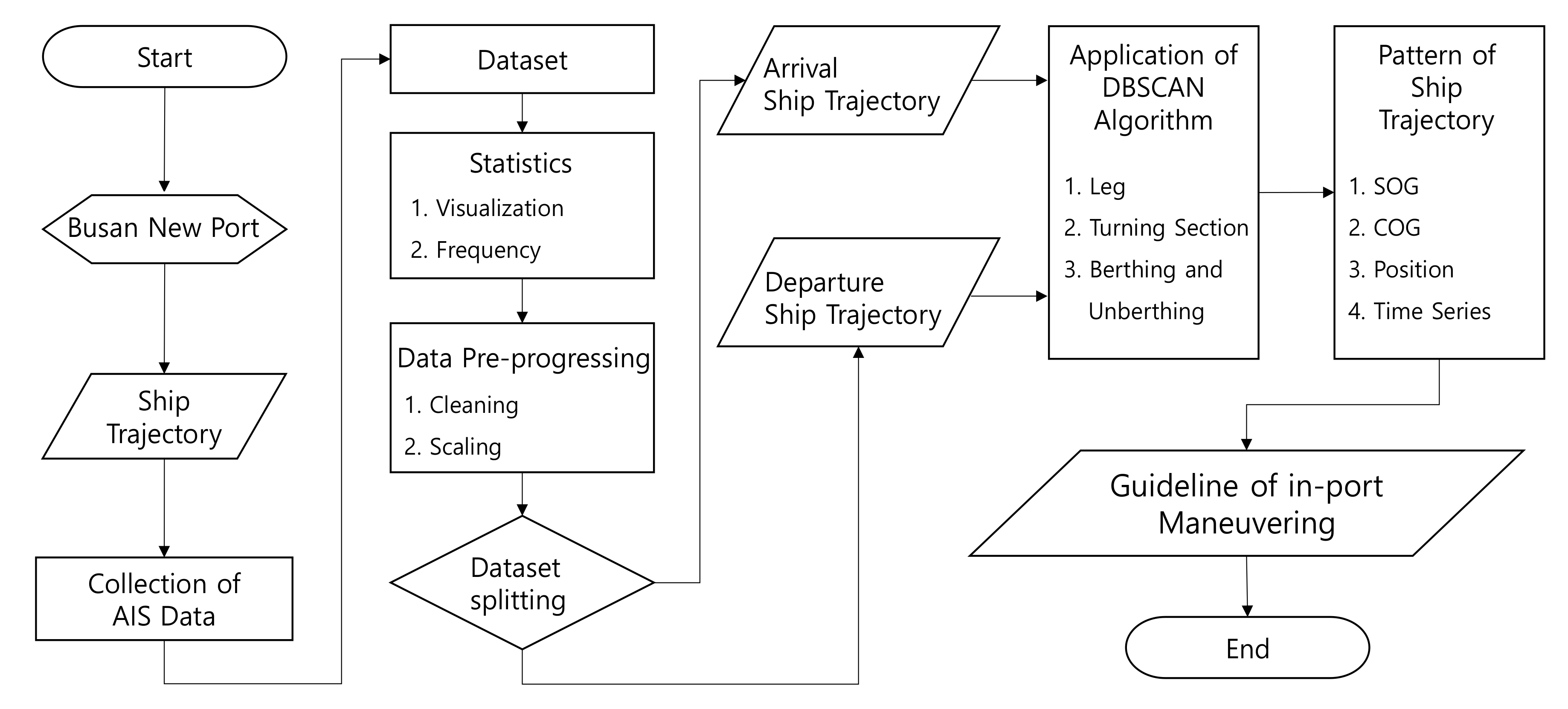
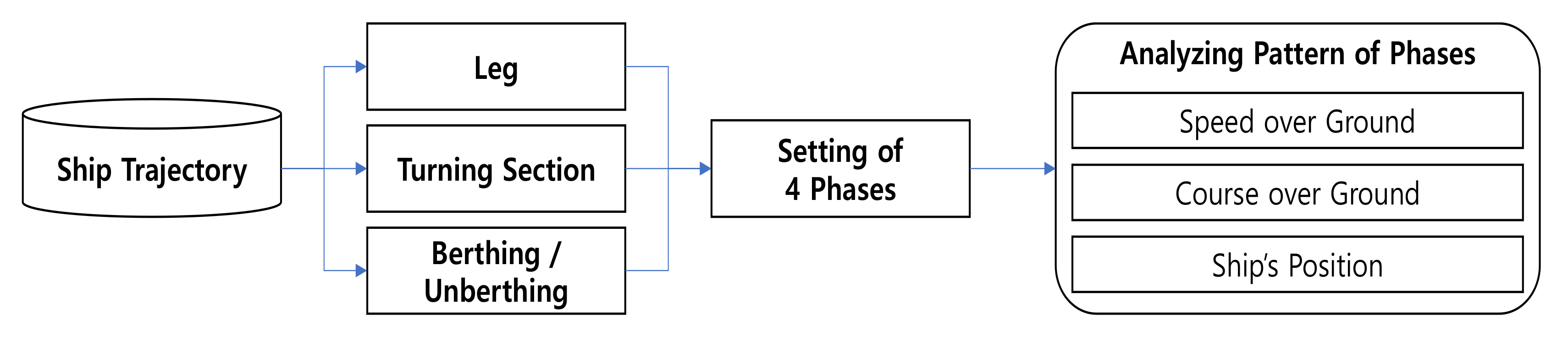
Figure 1.
Flowchart of the study.
Figure 1.
Flowchart of the study.
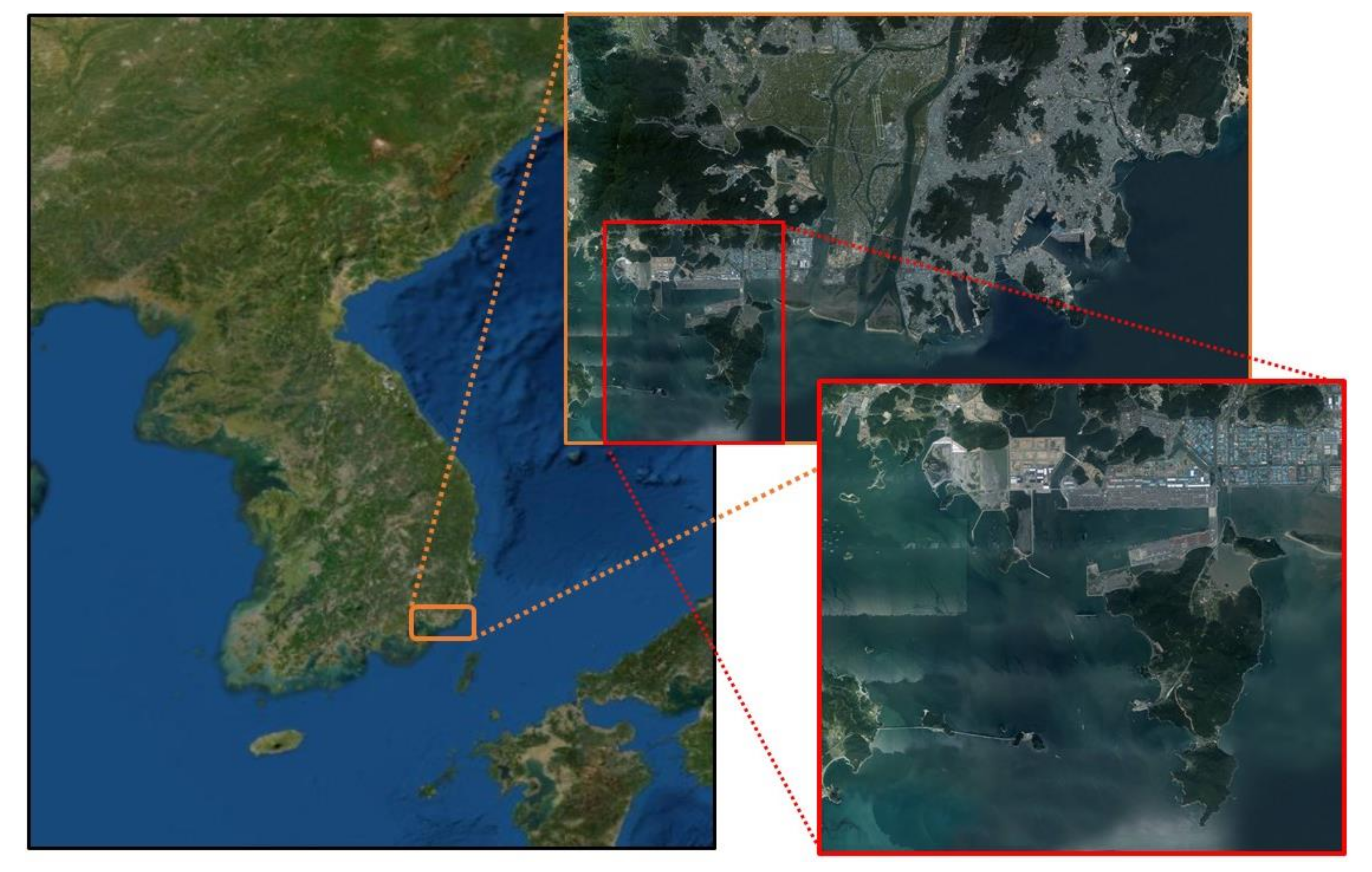
Figure 2.
Geographical location of Busan New Port in the Korea.
Figure 2.
Geographical location of Busan New Port in the Korea.
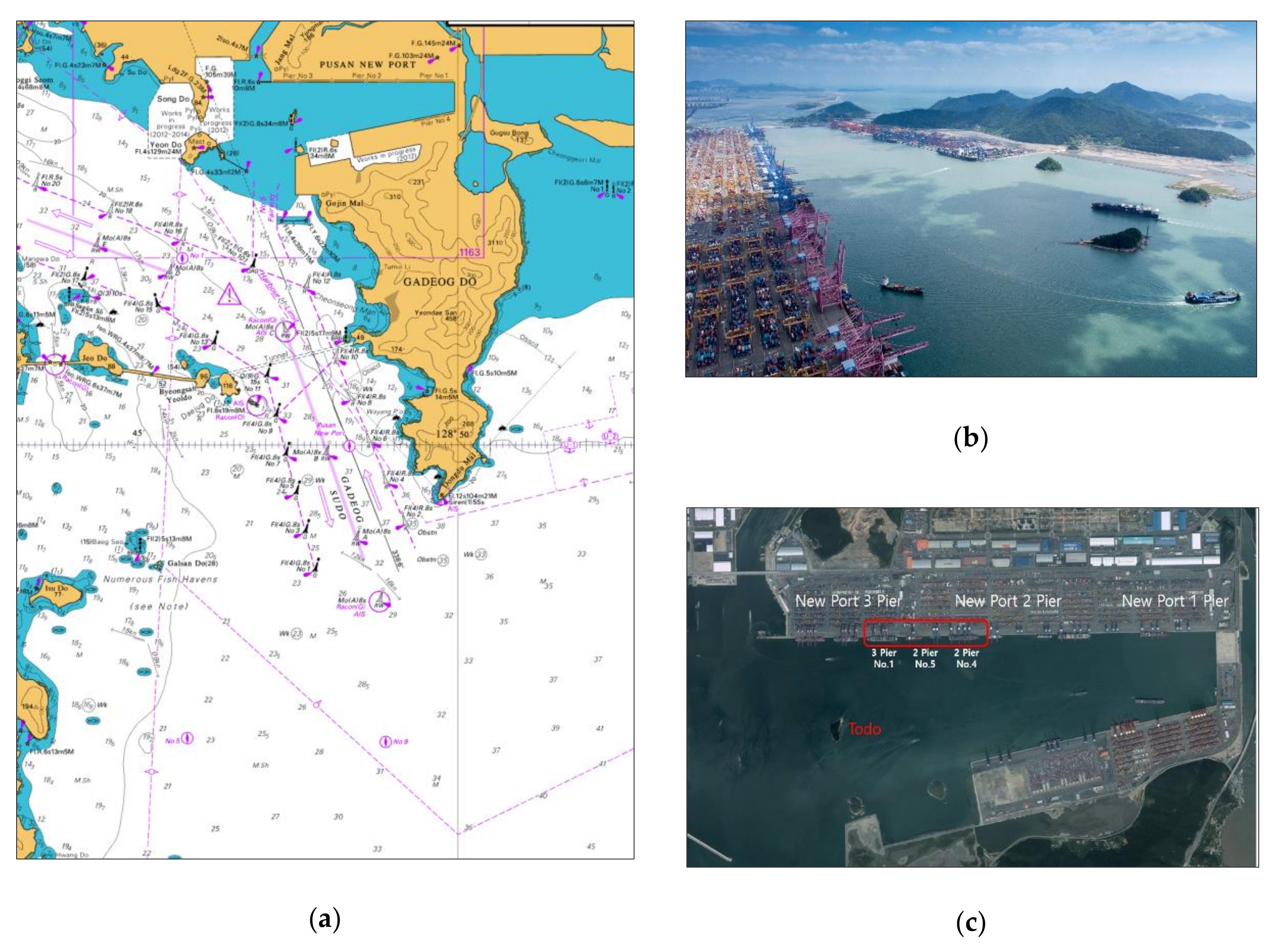
Figure 3.
Topographical characteristics of Busan New Port: (a) British Admiralty Chart; (b) ship passing around Todo island; (c) location of the target pier.
Figure 3.
Topographical characteristics of Busan New Port: (a) British Admiralty Chart; (b) ship passing around Todo island; (c) location of the target pier.
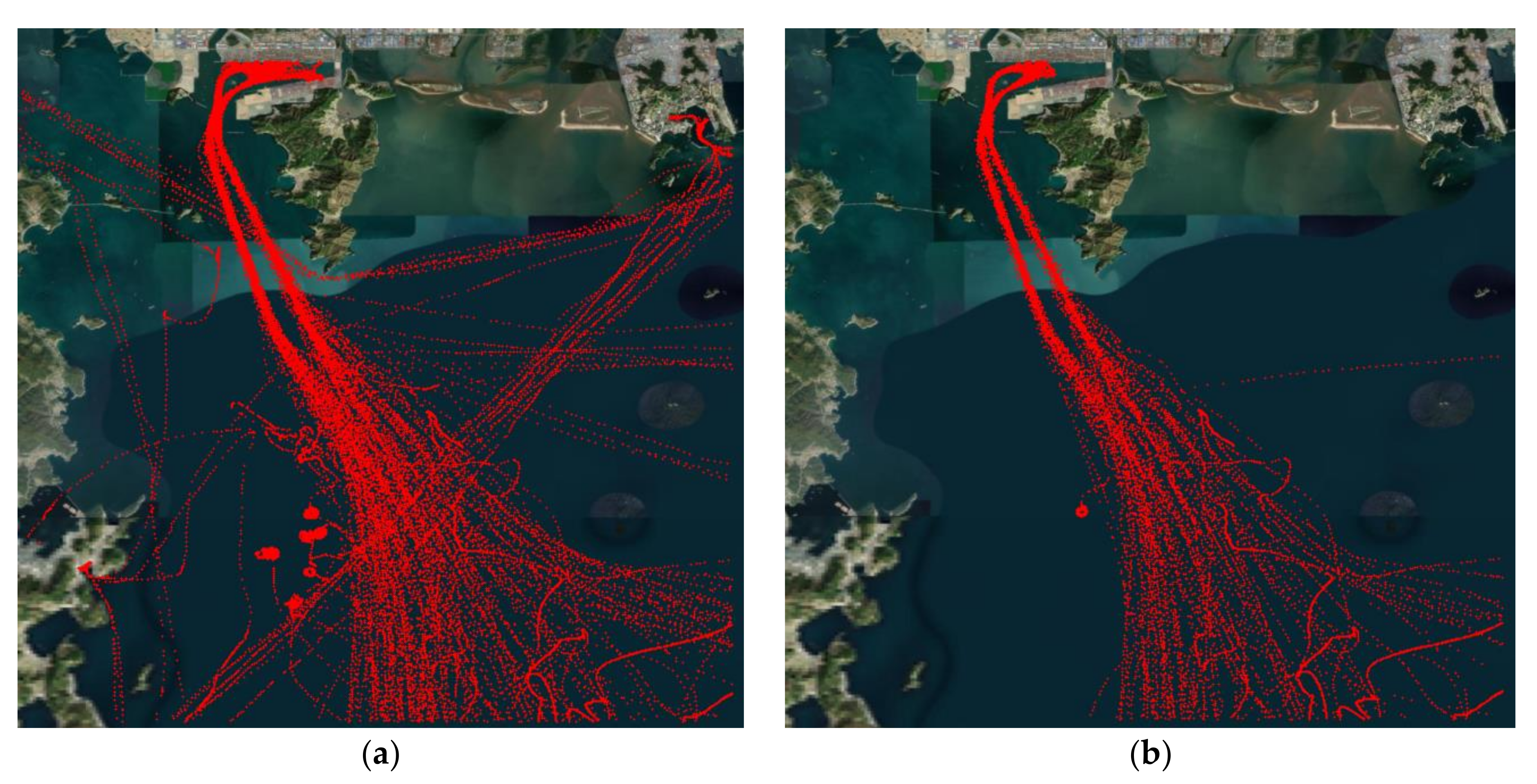
Figure 4.
Visualization of ship trajectory using AIS data: (a) raw data; (b) data to use for analysis.
Figure 4.
Visualization of ship trajectory using AIS data: (a) raw data; (b) data to use for analysis.
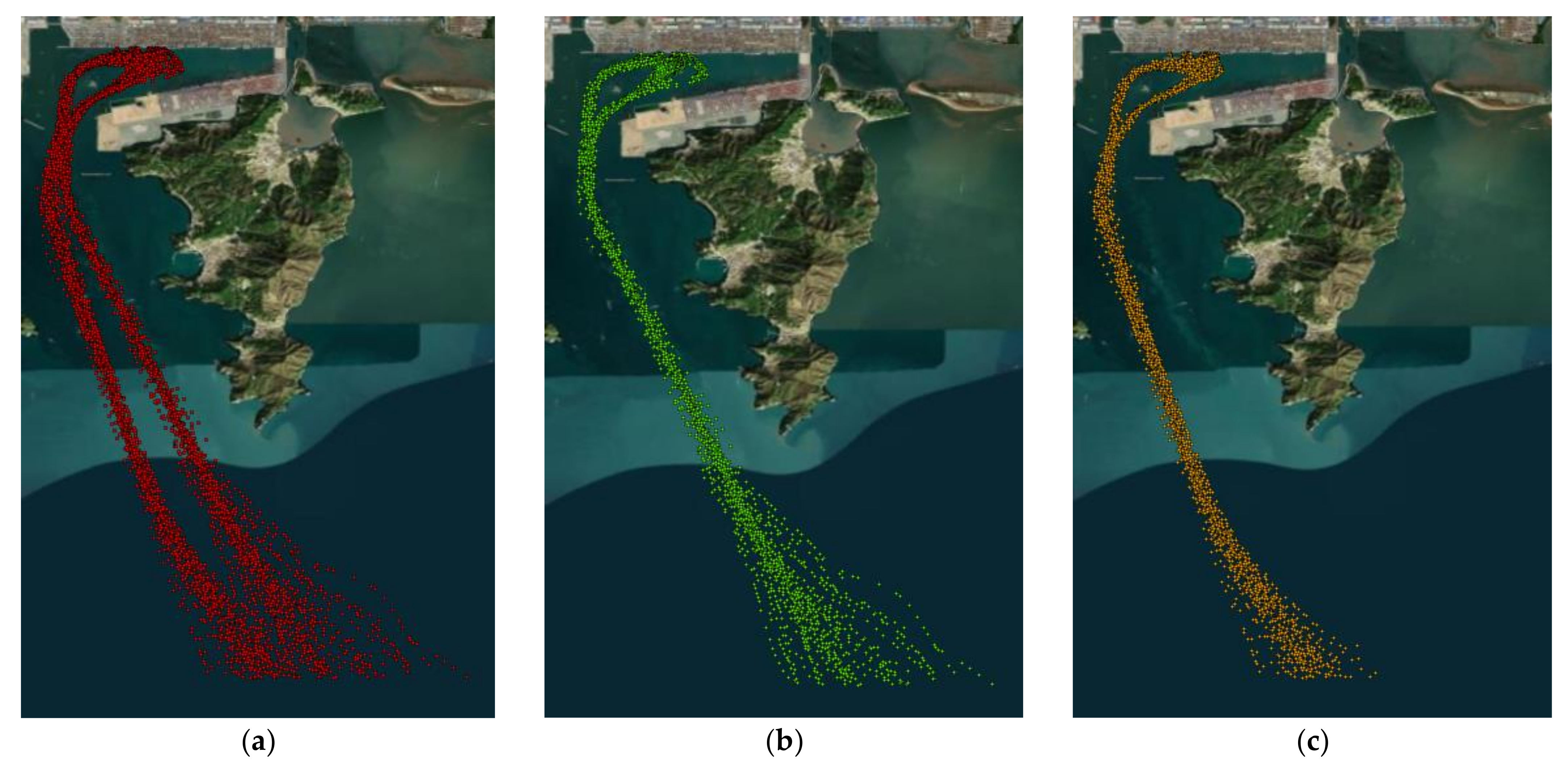
Figure 5.
Pre-processed AIS ship trajectory data: (a) all data; (b) arrival data; (c) departure data.
Figure 5.
Pre-processed AIS ship trajectory data: (a) all data; (b) arrival data; (c) departure data.
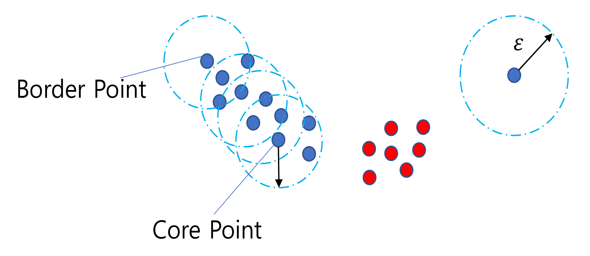
Figure 6.
Example of the density-based spatial clustering of applications with noise (DBSCAN) algorithm.
Figure 6.
Example of the density-based spatial clustering of applications with noise (DBSCAN) algorithm.
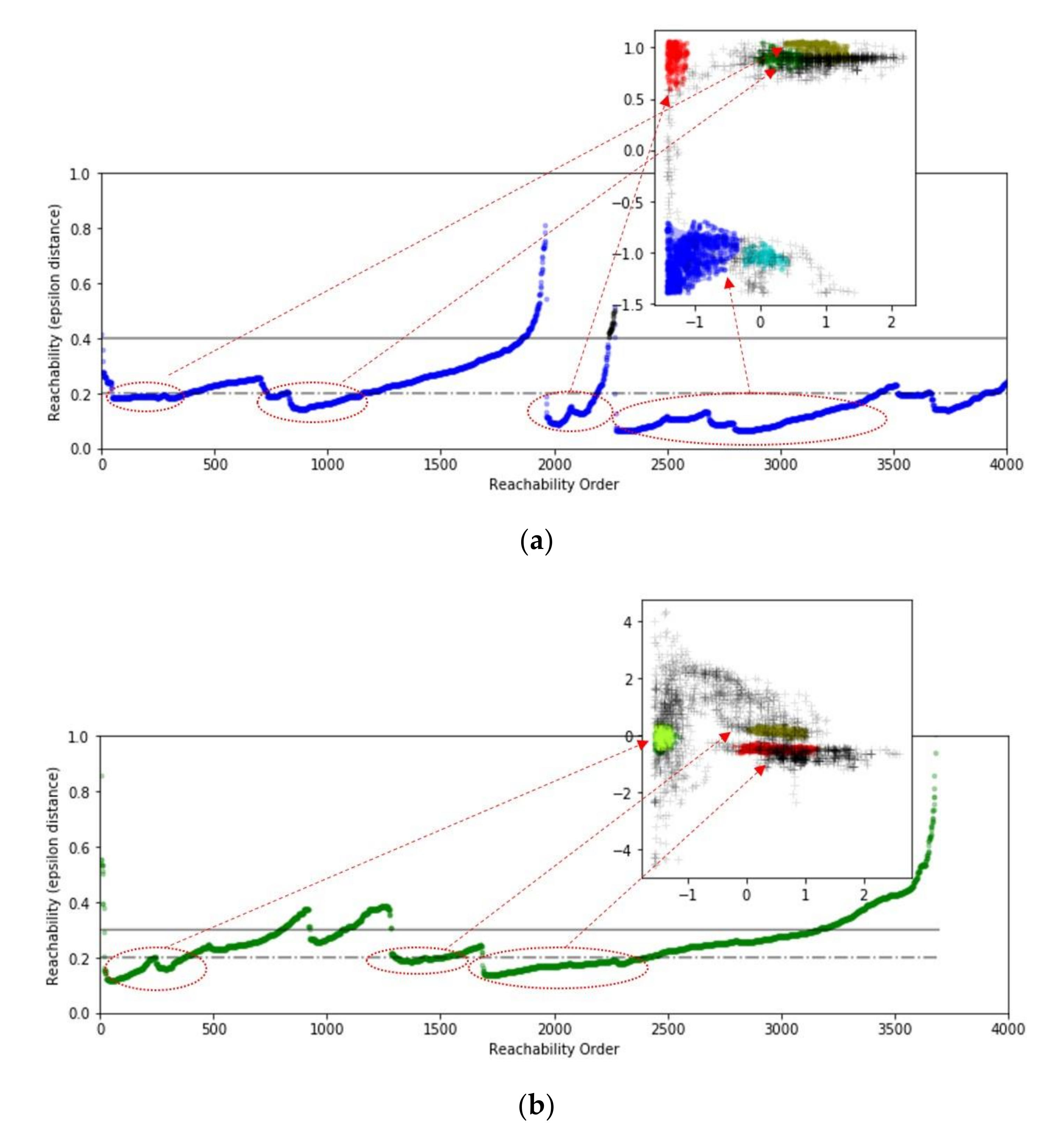
Figure 7.
Reachability plot: (a) arrival ship trajectory data; (b) departure ship trajectory data.
Figure 7.
Reachability plot: (a) arrival ship trajectory data; (b) departure ship trajectory data.
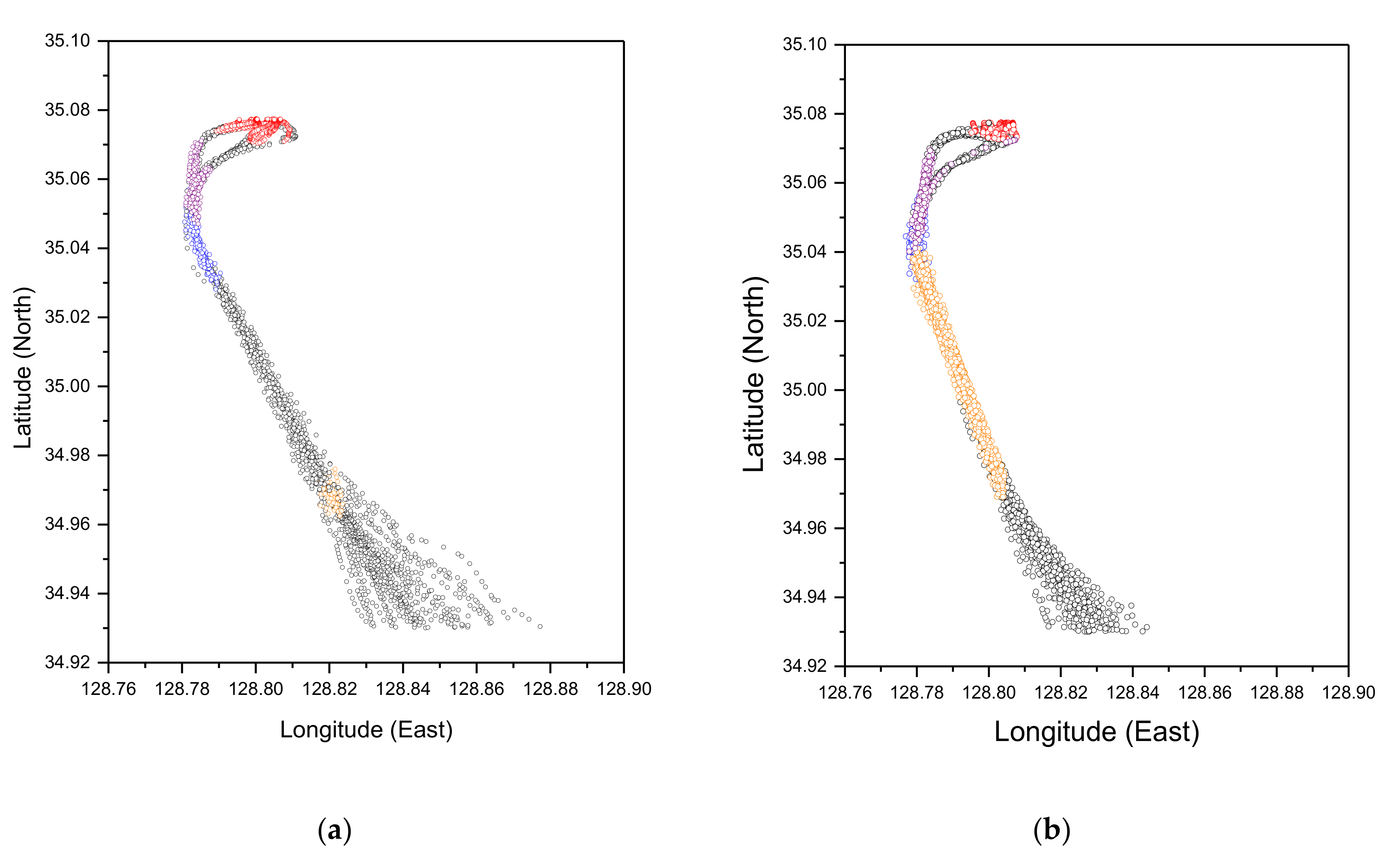
Figure 8.
Application of the DBSCAN algorithm: (a) arrival; (b) departure.
Figure 8.
Application of the DBSCAN algorithm: (a) arrival; (b) departure.
Figure 9.
Framework for analyzing the pattern of a ship’s trajectory.
Figure 9.
Framework for analyzing the pattern of a ship’s trajectory.
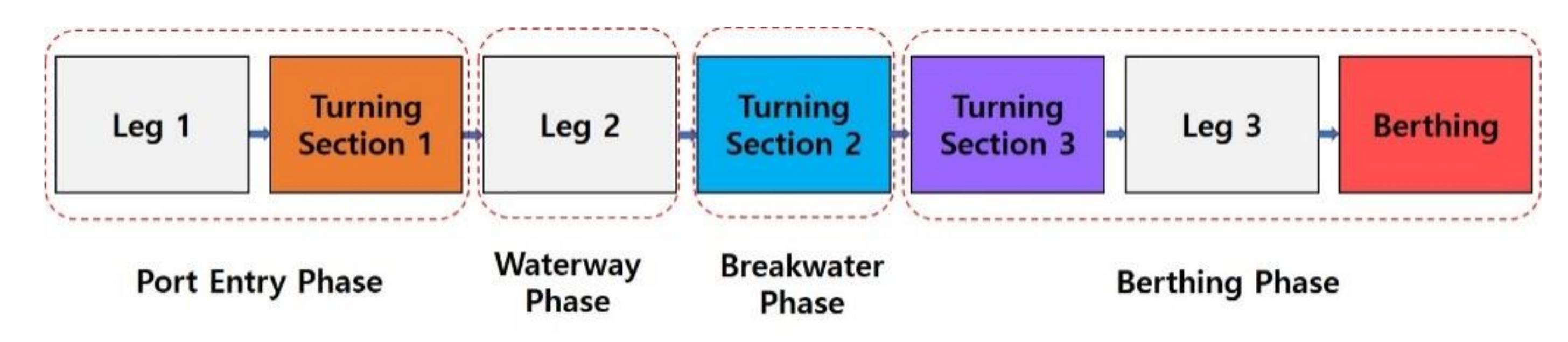
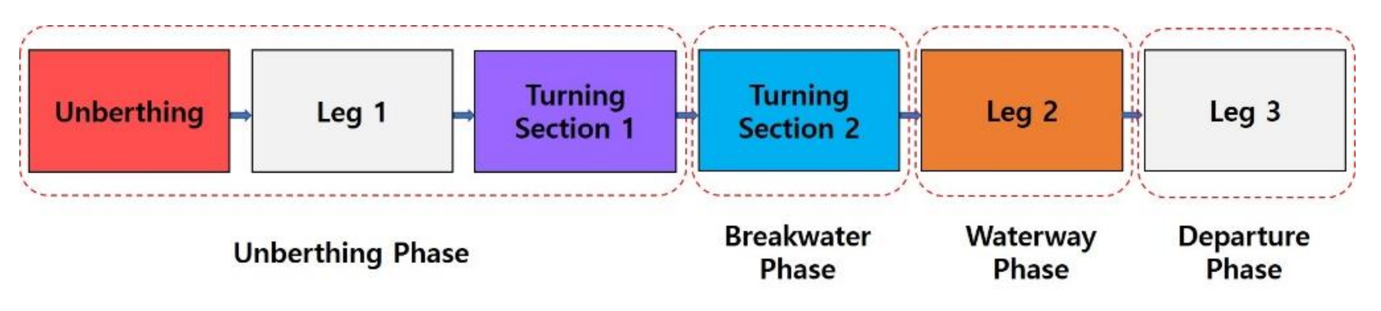
Figure 10.
Phase designation of the arrival cluster.
Figure 10.
Phase designation of the arrival cluster.
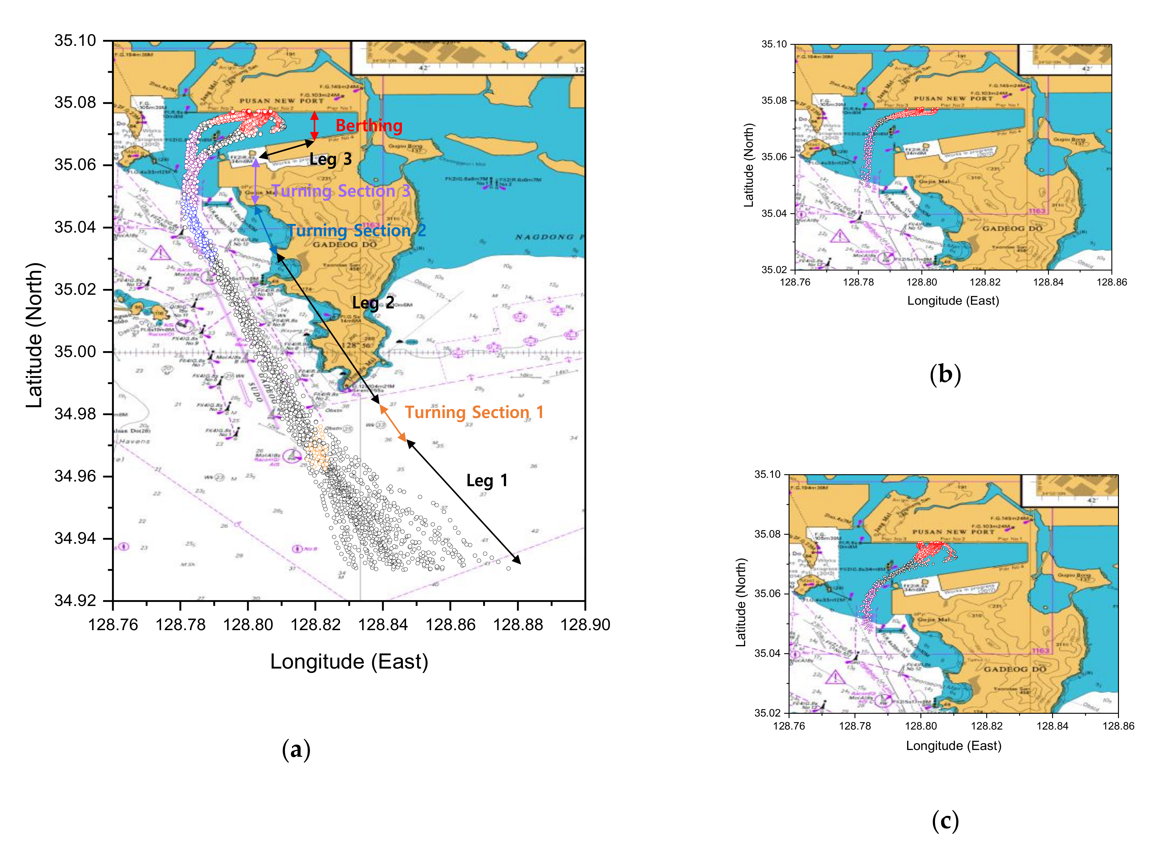
Figure 11.
Plotting the arriving ship’s trajectory data on the British Admiralty Chart: (a) all data; (b) passing the left side of Todo; and (c) passing the right side of Todo.
Figure 11.
Plotting the arriving ship’s trajectory data on the British Admiralty Chart: (a) all data; (b) passing the left side of Todo; and (c) passing the right side of Todo.
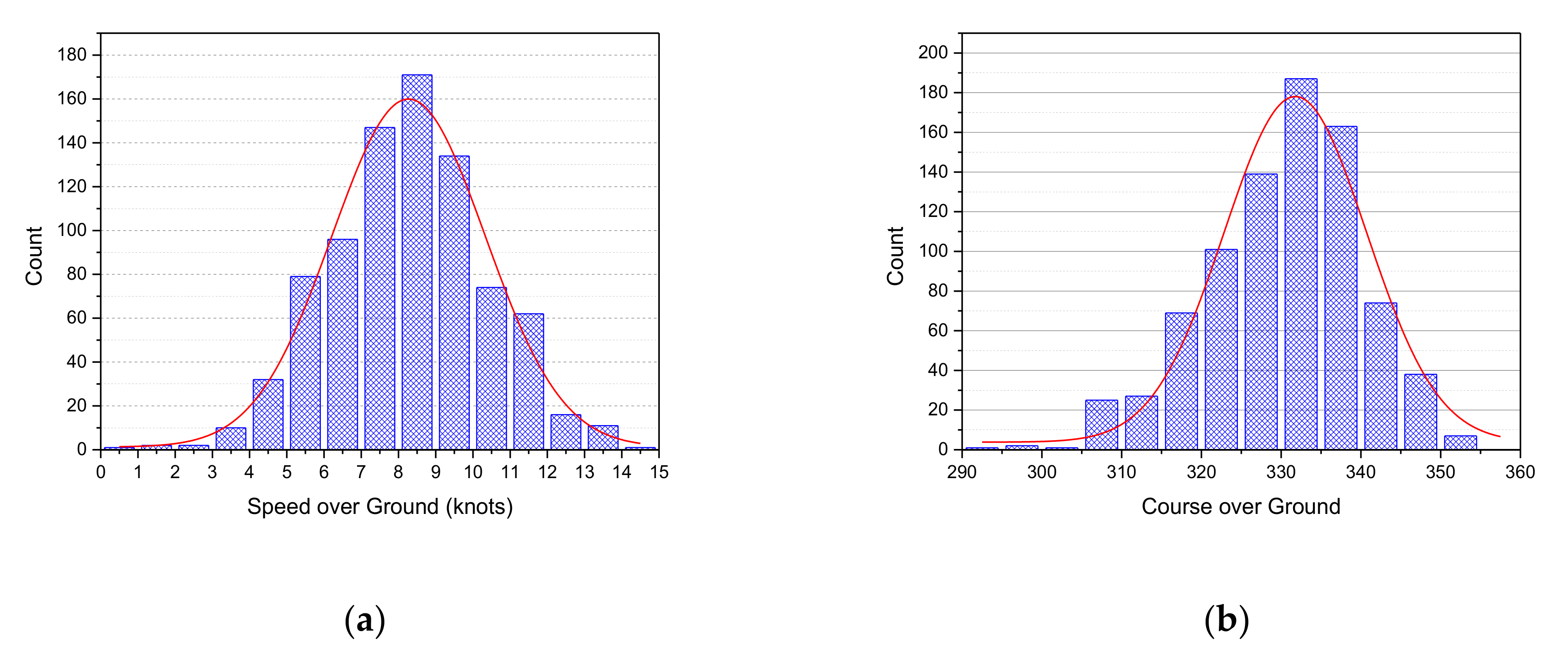
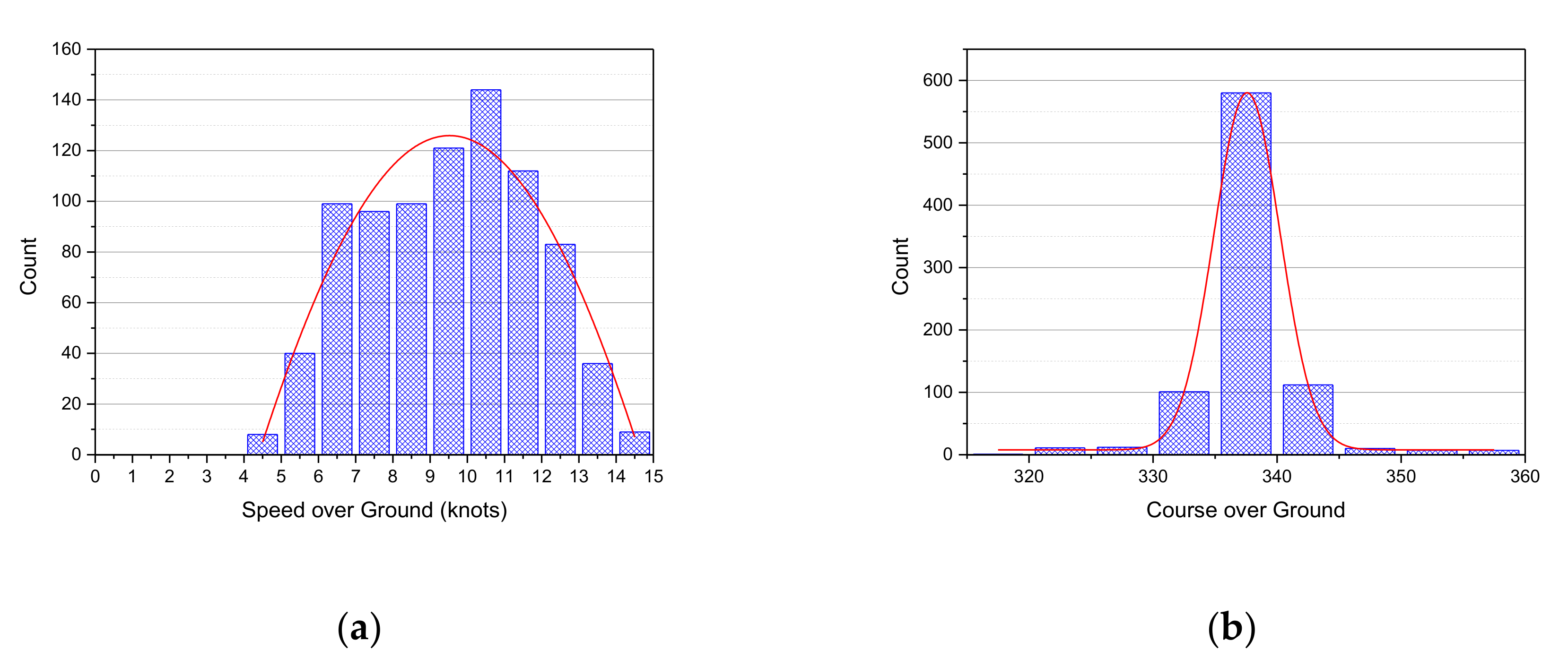
Figure 12.
Frequency analysis of the port entry phase: (a) speed over ground (SOG); (b) course over ground (COG).
Figure 12.
Frequency analysis of the port entry phase: (a) speed over ground (SOG); (b) course over ground (COG).
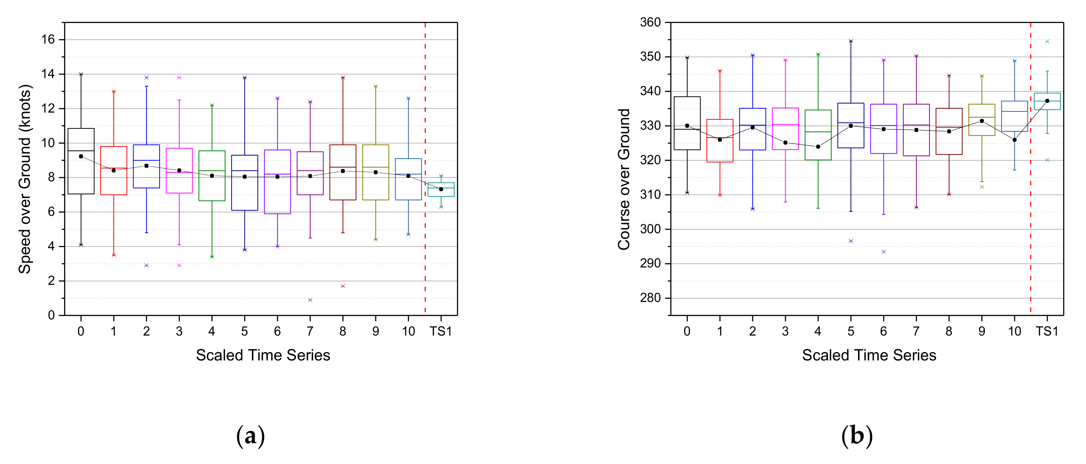
Figure 13.
Boxplot time series analysis of the port entry phase: (a) SOG; (b) COG; * the time series analysis for ship trajectories in Leg 1 is expressed in 11 stages, from 0 to 10, by multiplying the result scaled in Equation (1) by 10. This phase is expressed as a 12 stages time series graph by adding a Turning Section 1 in addition to Leg 1 divided into 11 stages. The boxplot was used to visually express the descriptive statistics for 12 stages.
Figure 14.
Frequency analysis of the waterway phase: (a) SOG; (b) COG.
Figure 14.
Frequency analysis of the waterway phase: (a) SOG; (b) COG.
Figure 15.
Boxplot time analysis of the arrival waterway phase: (a) SOG; (b) COG; * the time series analysis for ship trajectories in this phase is expressed in 11 stages, from 0 to 10, by multiplying the result scaled in Equation (1) by 10. In addition, the boxplot was used to visually express the descriptive statistics for 11 stages.
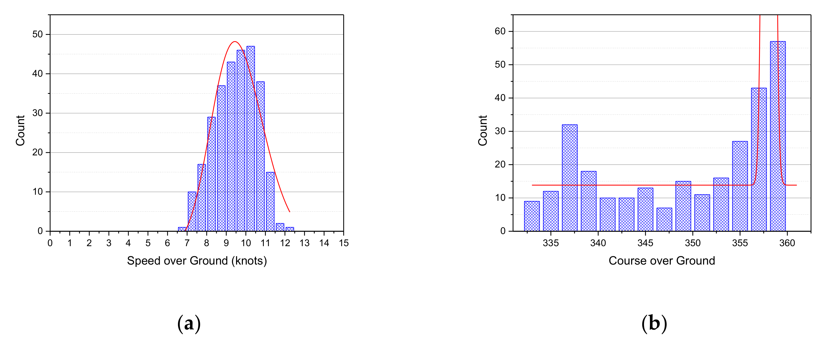
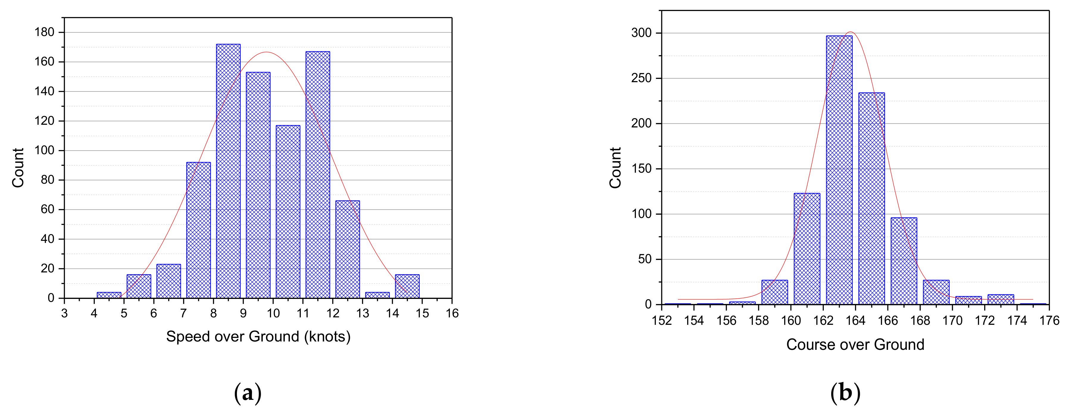
Figure 16.
Frequency analysis of the arrival breakwater phase: (a) SOG; (b) COG.
Figure 16.
Frequency analysis of the arrival breakwater phase: (a) SOG; (b) COG.
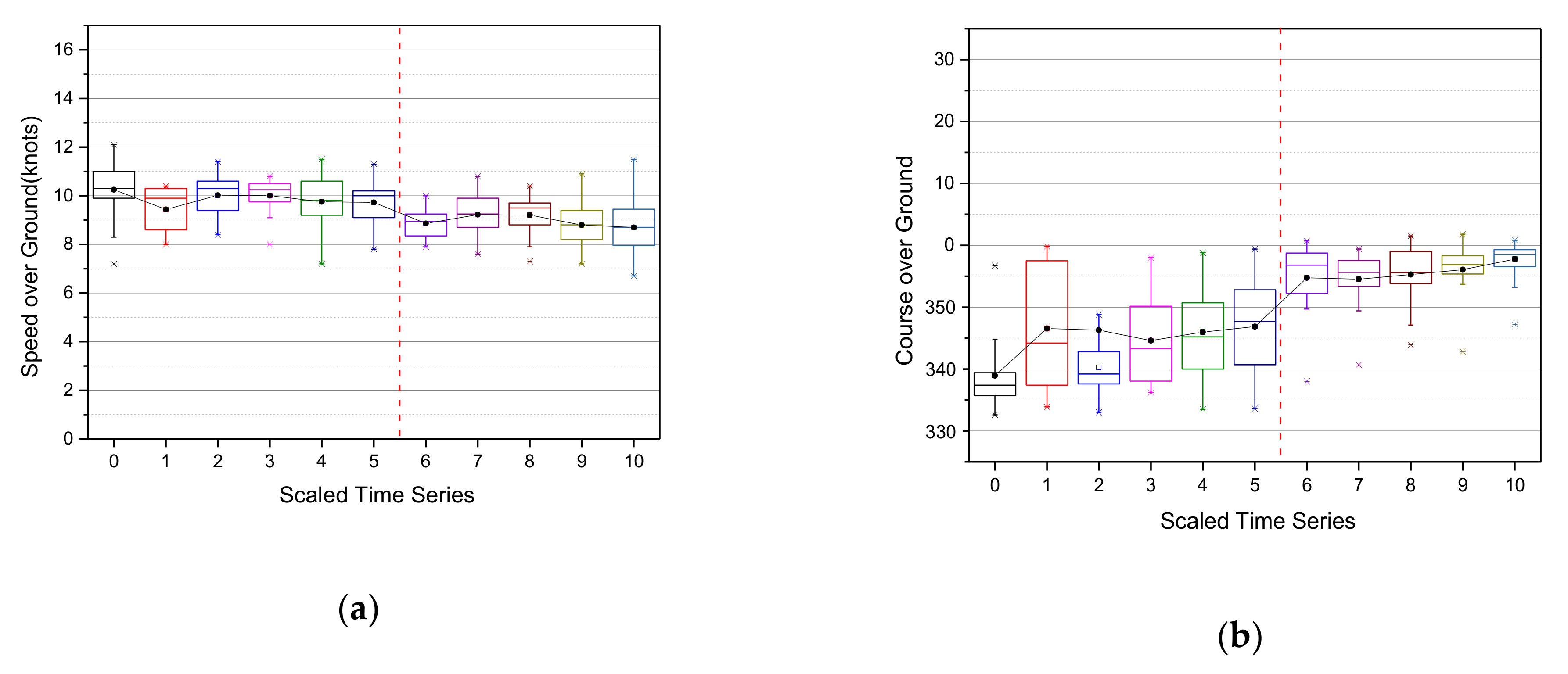
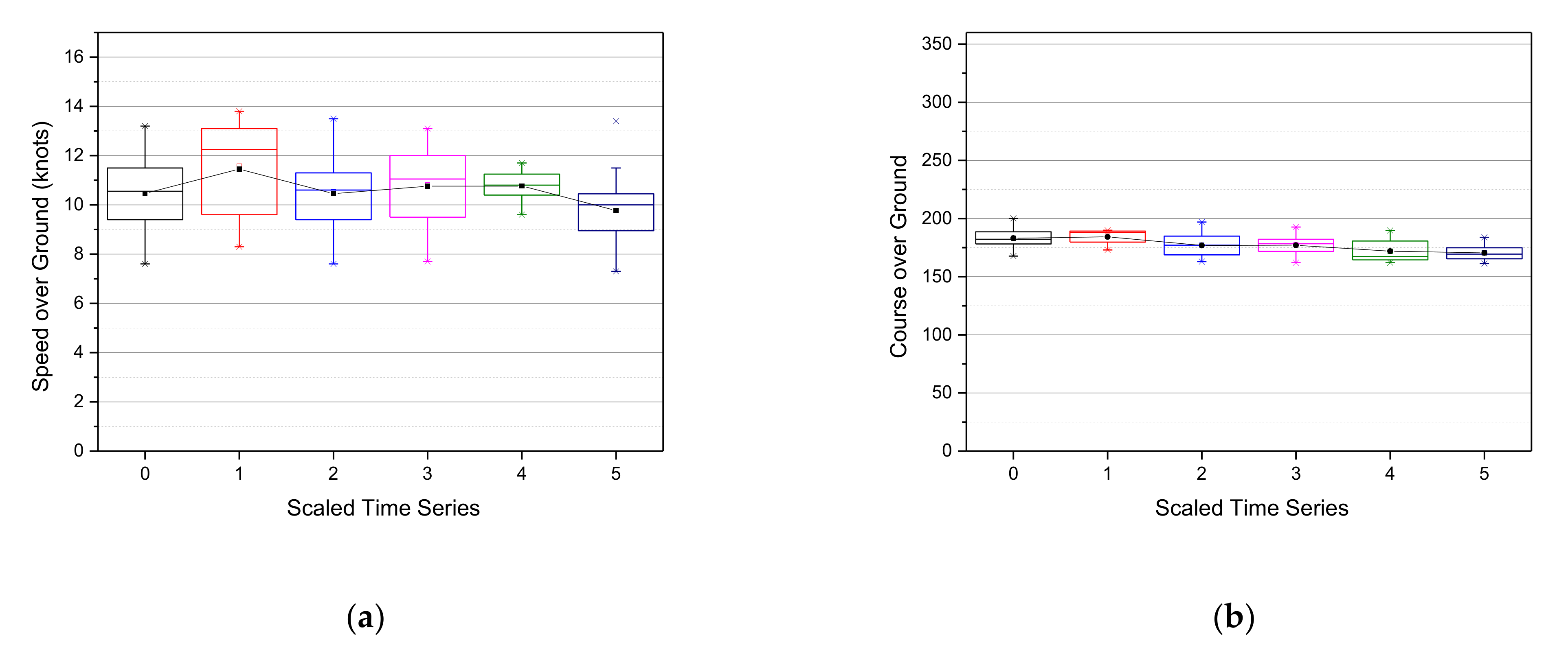
Figure 17.
Boxplot time series analysis of the arrival breakwater phase: (a) SOG; (b) COG; * the time series analysis for ship trajectories in this phase is expressed in 11 stages, from 0 to 10, by multiplying the result scaled in Equation (1) by 10. In addition, the boxplot was used to visually express the descriptive statistics for 11 stages.
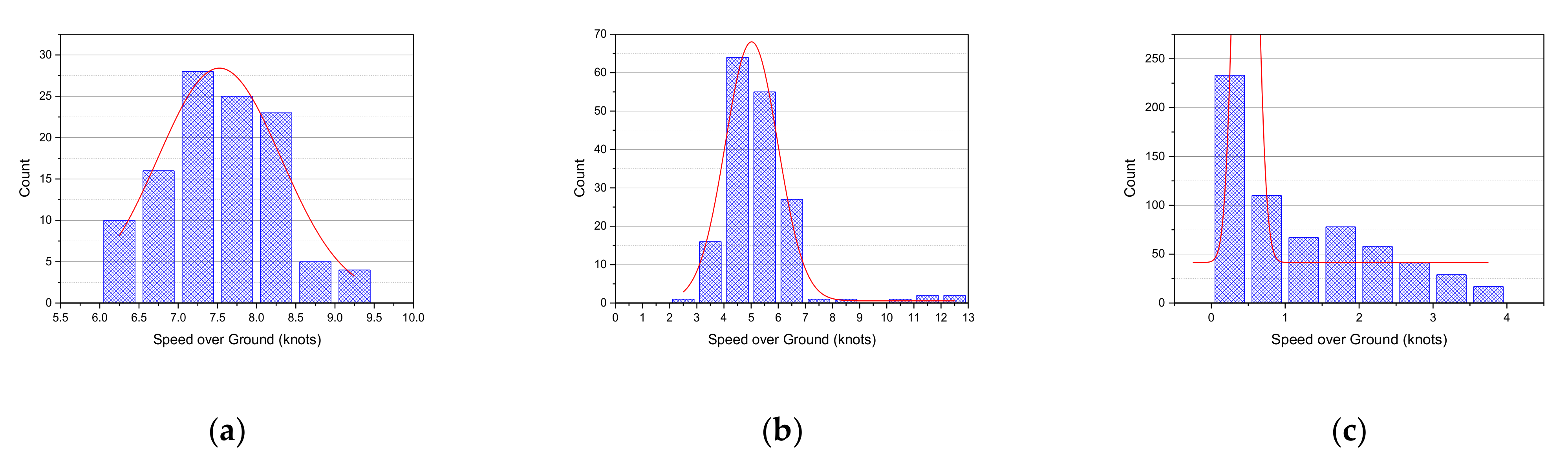
Figure 18.
Frequency analysis of the SOG on the left-side berthing phase: (a) Turning Section 3; (b) Leg 3; and (c) Berthing.
Figure 18.
Frequency analysis of the SOG on the left-side berthing phase: (a) Turning Section 3; (b) Leg 3; and (c) Berthing.
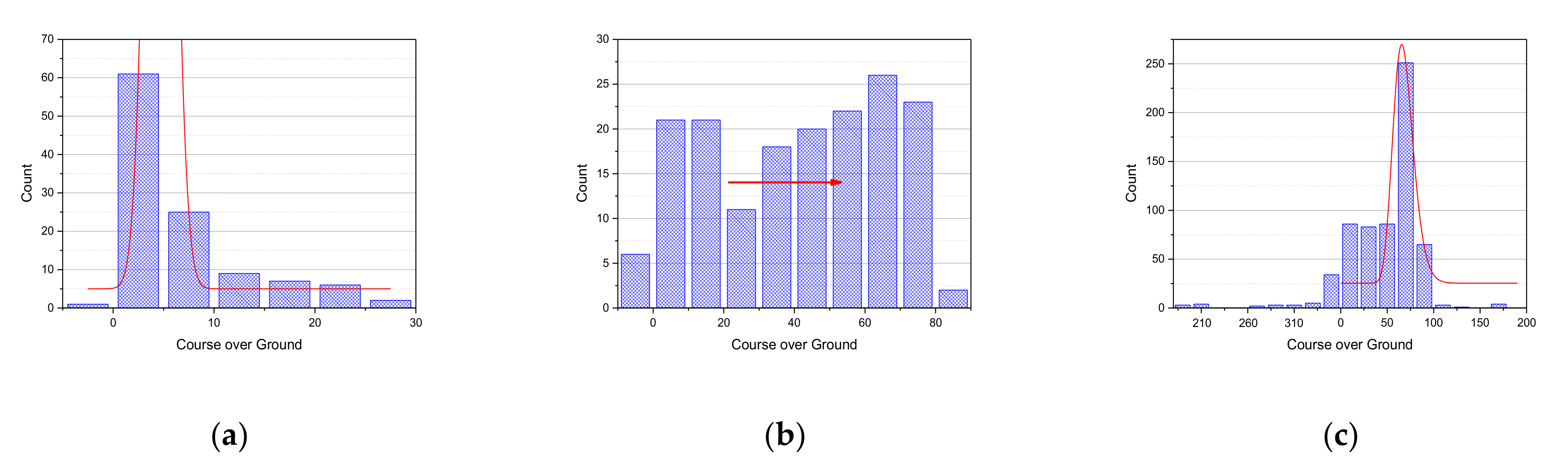
Figure 19.
Frequency analysis for the COG of the left-side berthing phase: (a) Turning Section 3; (b) Leg 3; and (c) Berthing.
Figure 19.
Frequency analysis for the COG of the left-side berthing phase: (a) Turning Section 3; (b) Leg 3; and (c) Berthing.
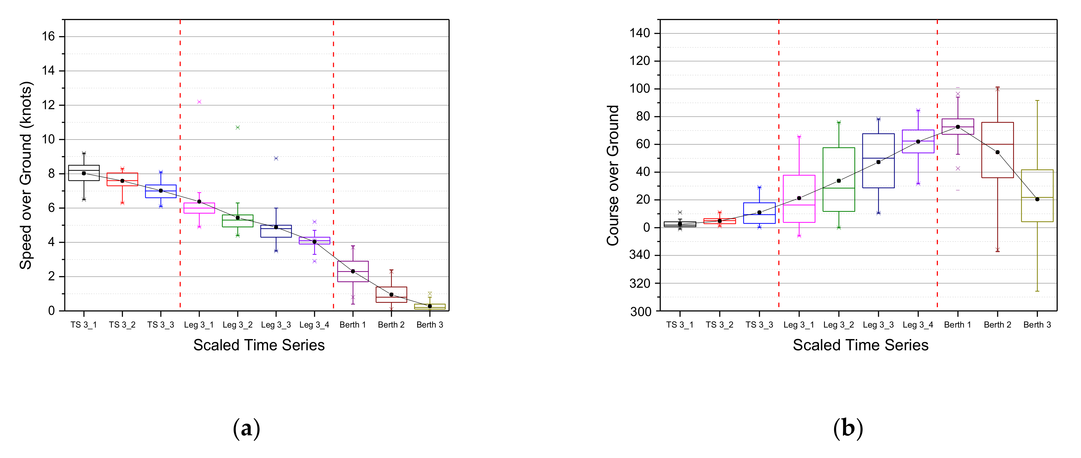
Figure 20.
Boxplot time series of the berthing phase passing Todo on the left: (a) SOG; (b) COG; * the time series analysis for ship trajectories in the case of passing Todo on the left is expressed in 11 stages by multiplying the result scaled in Equation (1) by 10. It was divided into 3 stages in Turning Section 3 (TS 3), 4 stages in Leg 3, and 3 stages in Berth. In addition, the boxplot was used to visually express the descriptive statistics for 11 stages.
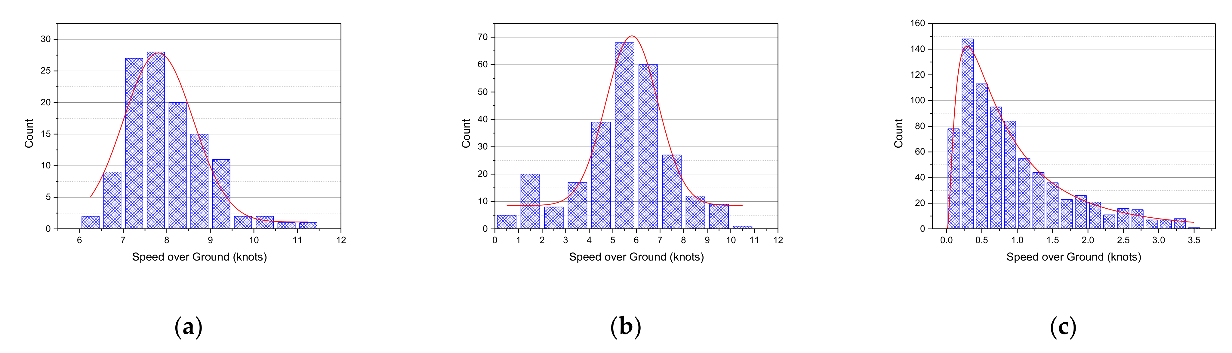
Figure 21.
Frequency analysis of the SOG of the right-side berthing phase: (a) Turning Section 3; (b) Leg 3; and (c) Berthing.
Figure 21.
Frequency analysis of the SOG of the right-side berthing phase: (a) Turning Section 3; (b) Leg 3; and (c) Berthing.
Figure 22.
Frequency analysis for the COG of the right-side berthing phase: (a) Turning Section 3; (b) Leg 3; and (c) Berthing.
Figure 22.
Frequency analysis for the COG of the right-side berthing phase: (a) Turning Section 3; (b) Leg 3; and (c) Berthing.
Figure 23.
Boxplot time series of the berthing phase passing through Todo on the right side: (a) SOG; (b) COG; * the time series analysis for ship trajectories in the case of passing Todo on the right is expressed in 11 stages by multiplying the result scaled in Equation (1) by 10. It was divided into 3 stages in Turning Section 3 (TS 3), 4 stages in Leg 3, and 3 stages in Berth. In addition, the boxplot was used to visually express the descriptive statistics for 11 stages.
Figure 24.
Phase designation of the departure cluster.
Figure 24.
Phase designation of the departure cluster.
Figure 25.
Plotting departing ships’ trajectory data on the British Admiralty Chart: (a) all data; (b) passing on left side of Todo; and (c) passing on right side of Todo.
Figure 25.
Plotting departing ships’ trajectory data on the British Admiralty Chart: (a) all data; (b) passing on left side of Todo; and (c) passing on right side of Todo.
Figure 26.
Frequency analysis for the SOG of the left side unberthing phase: (a) Unberthing; (b) Leg 1; and (c) Turning Section 1.
Figure 26.
Frequency analysis for the SOG of the left side unberthing phase: (a) Unberthing; (b) Leg 1; and (c) Turning Section 1.
Figure 27.
Frequency analysis for the COG of the left side unberthing phase: (a) Unberthing; (b) Leg 1; and (c) Turning Section 1.
Figure 27.
Frequency analysis for the COG of the left side unberthing phase: (a) Unberthing; (b) Leg 1; and (c) Turning Section 1.
Figure 28.
Boxplot time series of the unberthing phase passing through Todo to the left: (a) SOG; (b) COG; * the time series analysis for ship trajectories in the case of passing Todo on the left is expressed in 11 stages by multiplying the result scaled in Equation (1) by 10. It was divided into 3 stages in Unberth, 4 stages in Leg 1, and 3 stages in Turning Section 1 (TS 1). In addition, the boxplot was used to visually express the descriptive statistics for 11 stages.
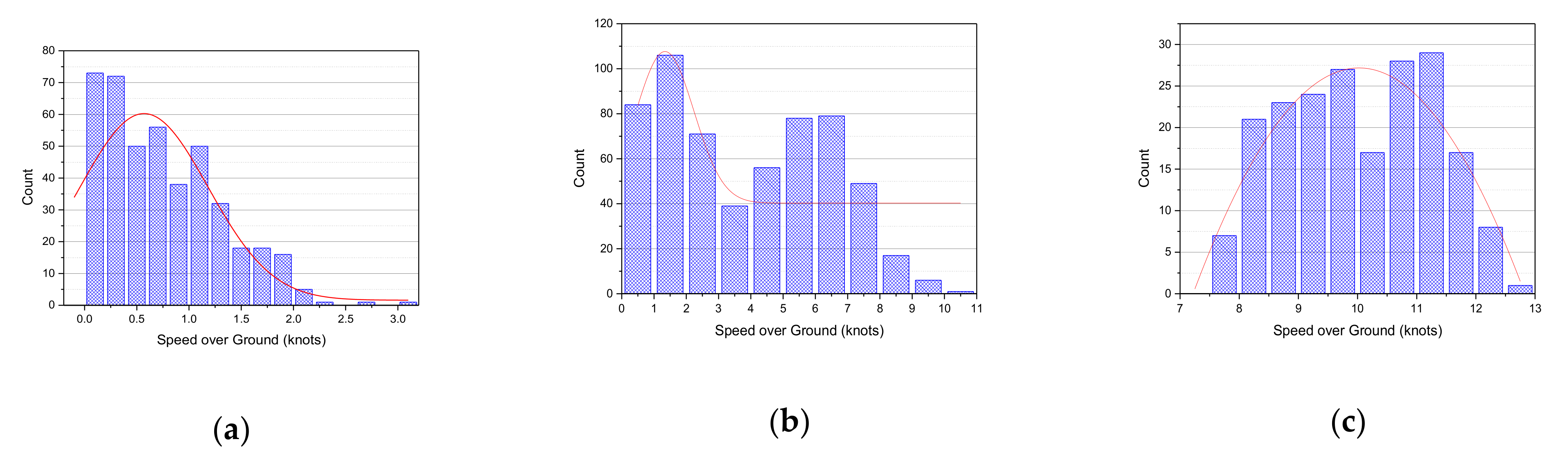
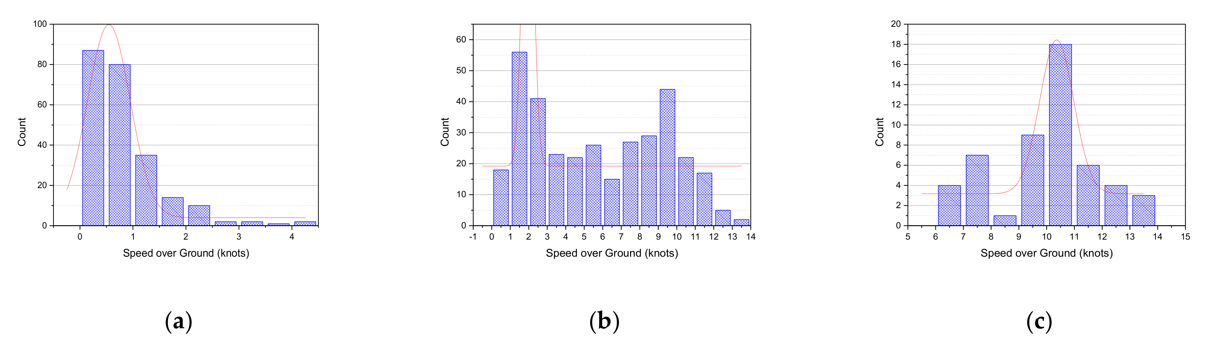
Figure 29.
Frequency analysis for the SOG of the right-side unberthing phase: (a) Unberthing; (b) Leg 1; and (c) Turning Section 1.
Figure 29.
Frequency analysis for the SOG of the right-side unberthing phase: (a) Unberthing; (b) Leg 1; and (c) Turning Section 1.
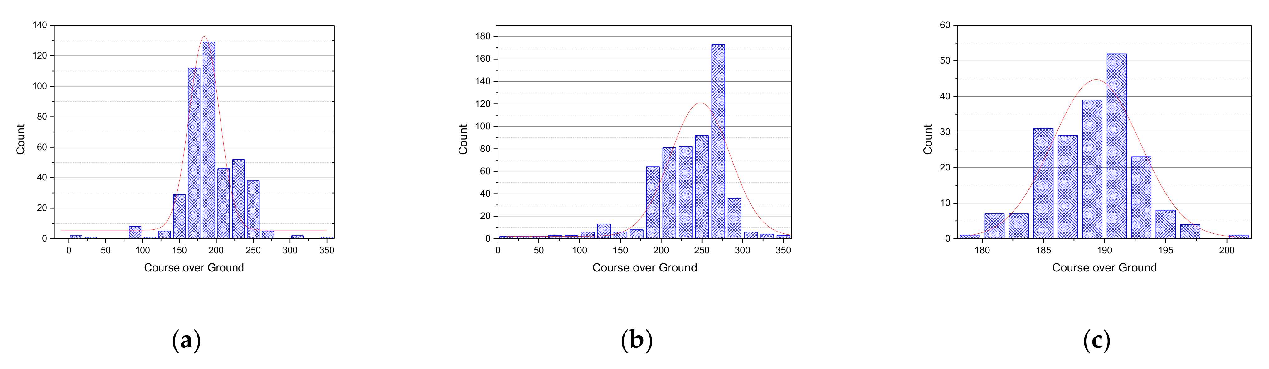
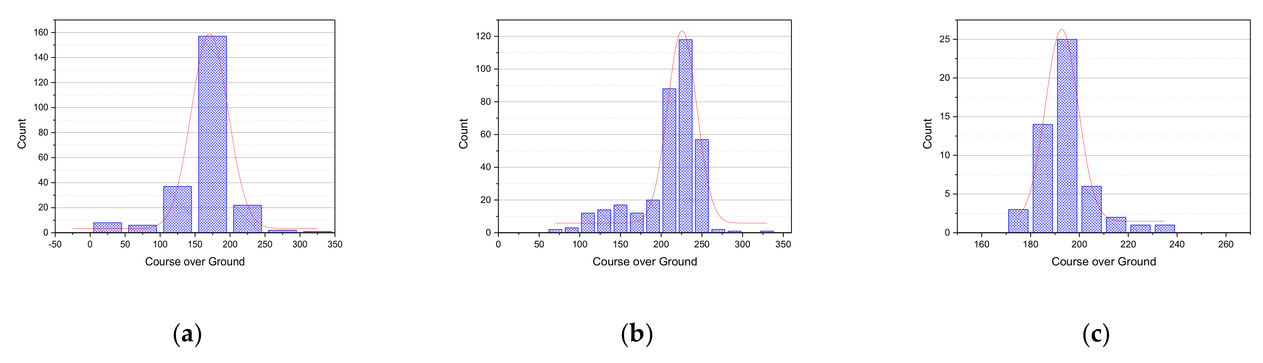
Figure 30.
Frequency analysis of the COG during the right-side unberthing phase: (a) Unberthing; (b) Leg 1; and (c) Turning Section 1.
Figure 30.
Frequency analysis of the COG during the right-side unberthing phase: (a) Unberthing; (b) Leg 1; and (c) Turning Section 1.
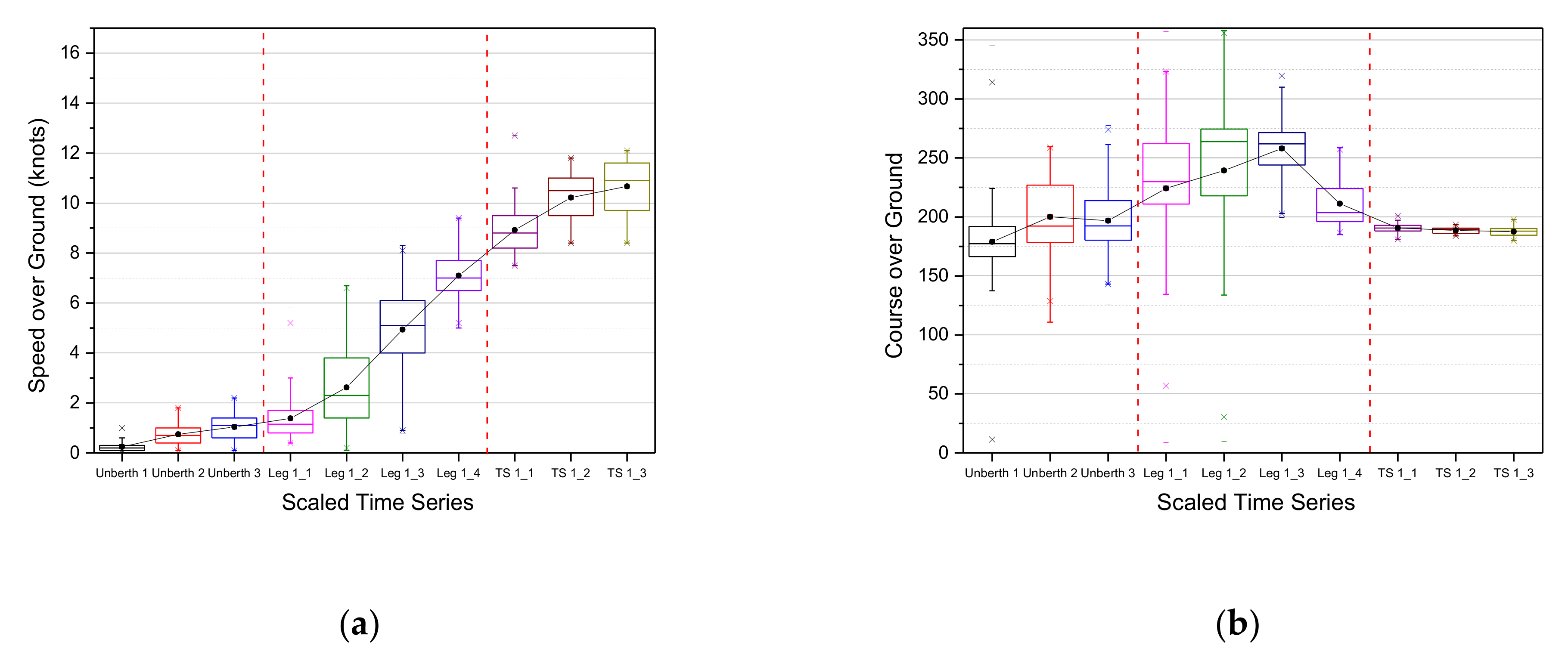
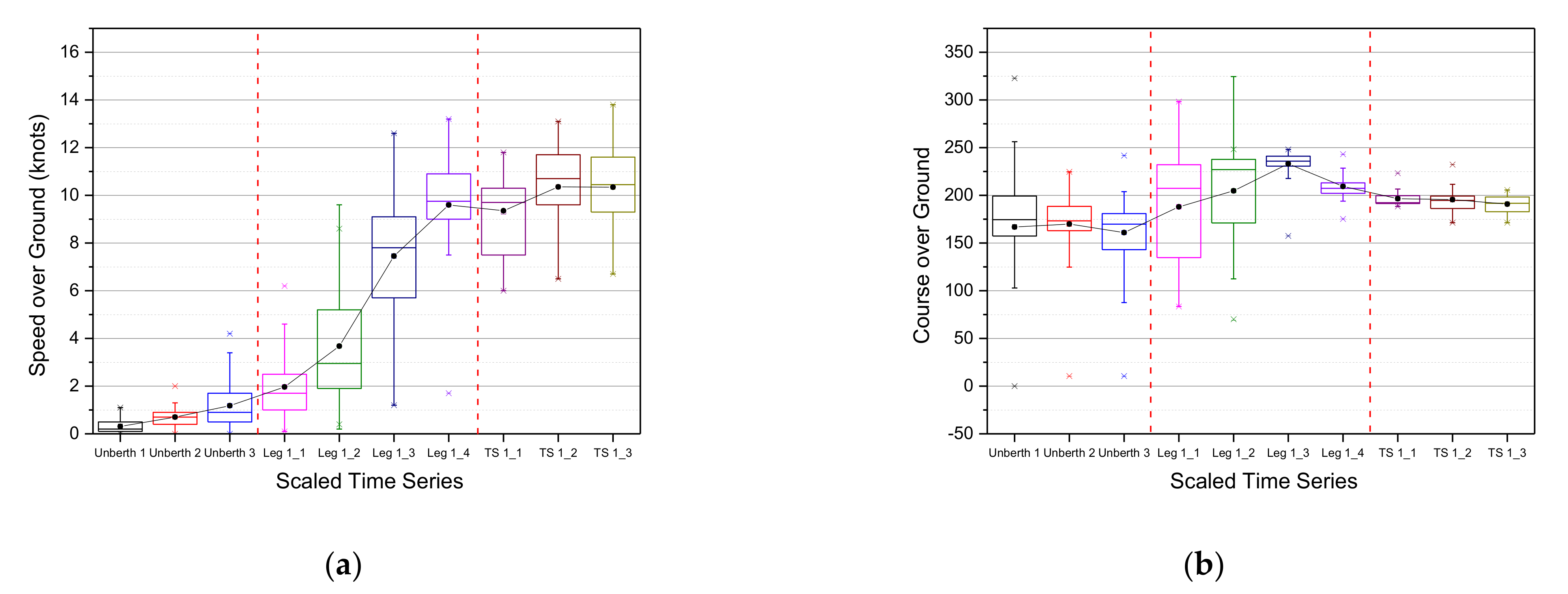
Figure 31.
Boxplot time series of the unberthing phase, passing Todo on the right: (a) SOG; (b) COG; * the time series analysis for ship trajectories in the case of passing Todo on the right is expressed in 11 stages by multiplying the result scaled in Equation (1) by 10. It was divided into 3 stages in Unberth, 4 stages in Leg 1, and 3 stages in Turning Section 1 (TS 1). In addition, the boxplot was used to visually express the descriptive statistics for 11 stages.
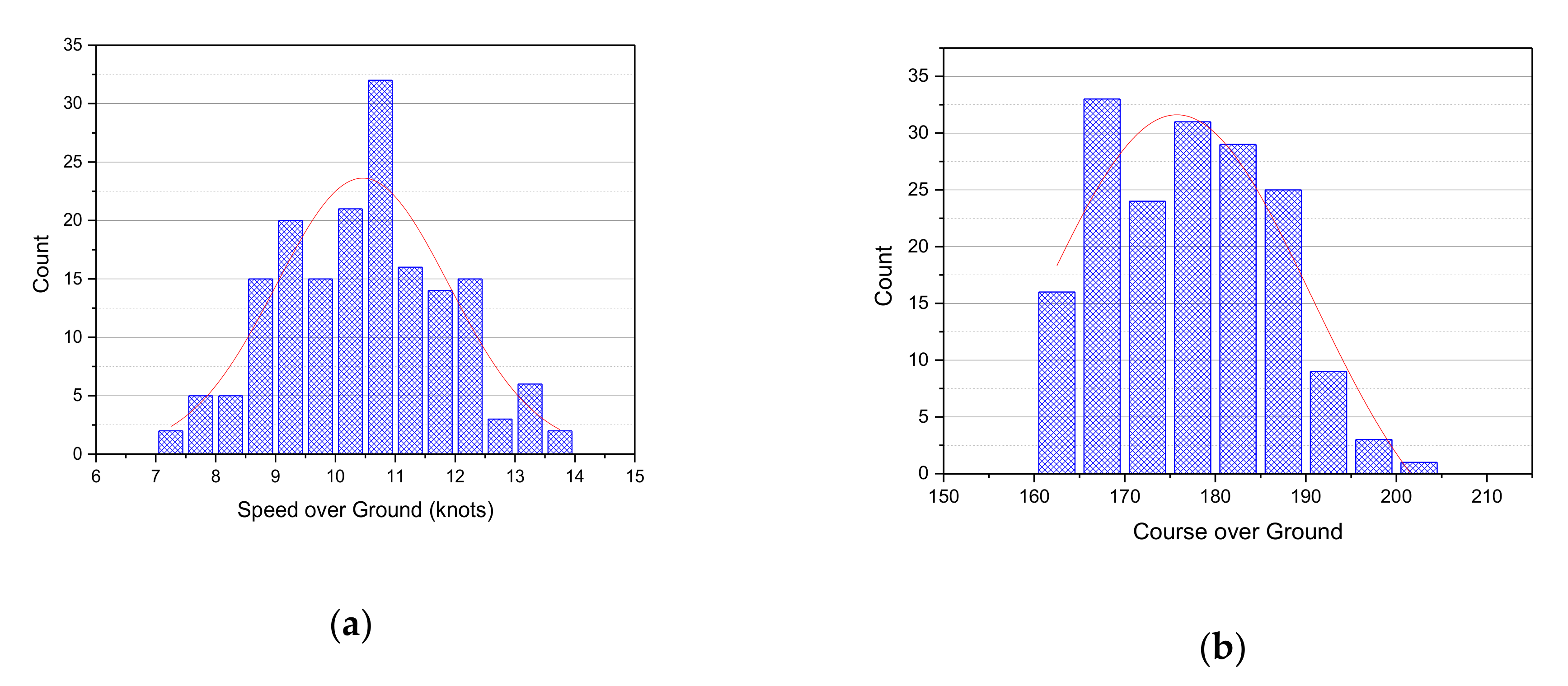
Figure 32.
Frequency analysis of the departure breakwater phase: (a) SOG; (b) COG.
Figure 32.
Frequency analysis of the departure breakwater phase: (a) SOG; (b) COG.
Figure 33.
Boxplot time series analysis of the departure breakwater phase: (
a) SOG; (
b) COG; * the time series analysis
Figure 6. stages, from 0 to 5, by multiplying the result scaled in Equation (1) by 10. In addition, the boxplot was used to visually express the descriptive statistics for 6 stages.
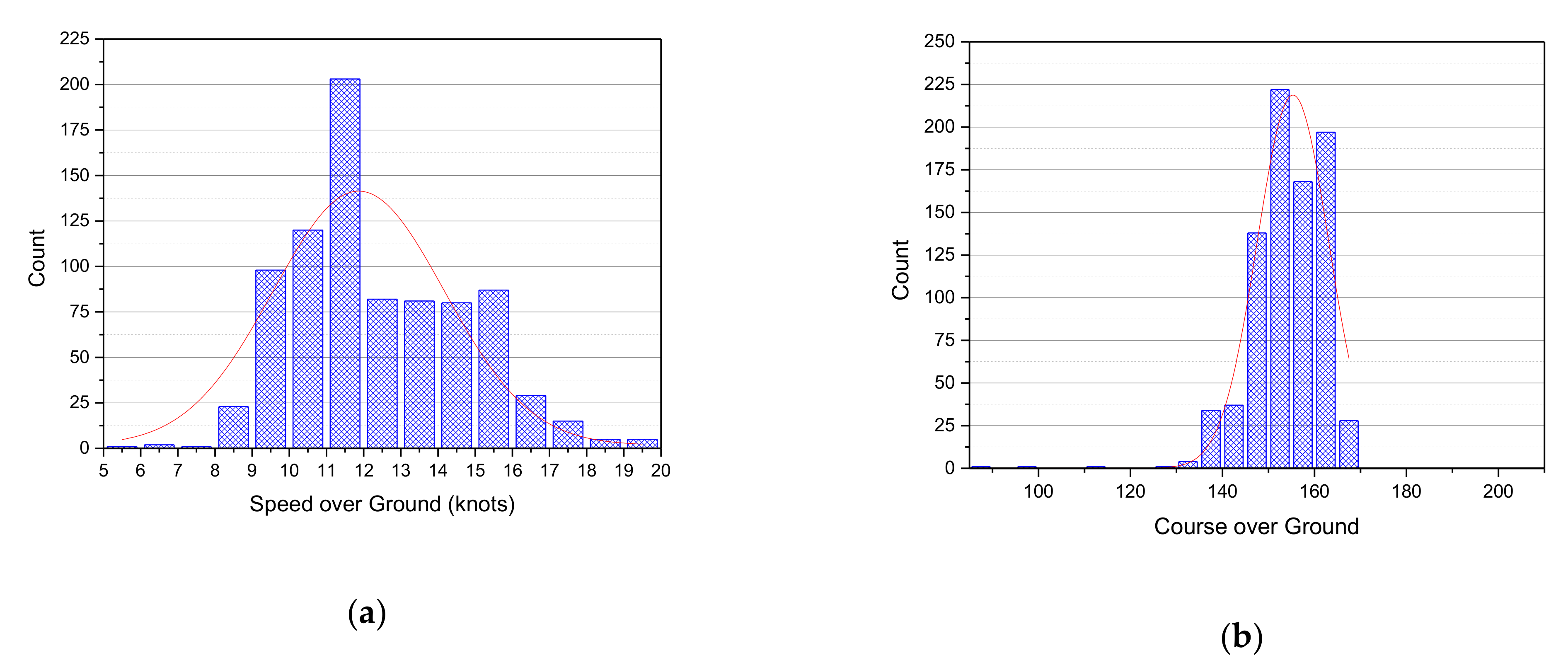
Figure 34.
Frequency analysis of the departure waterway phase: (a) SOG; (b) COG.
Figure 34.
Frequency analysis of the departure waterway phase: (a) SOG; (b) COG.
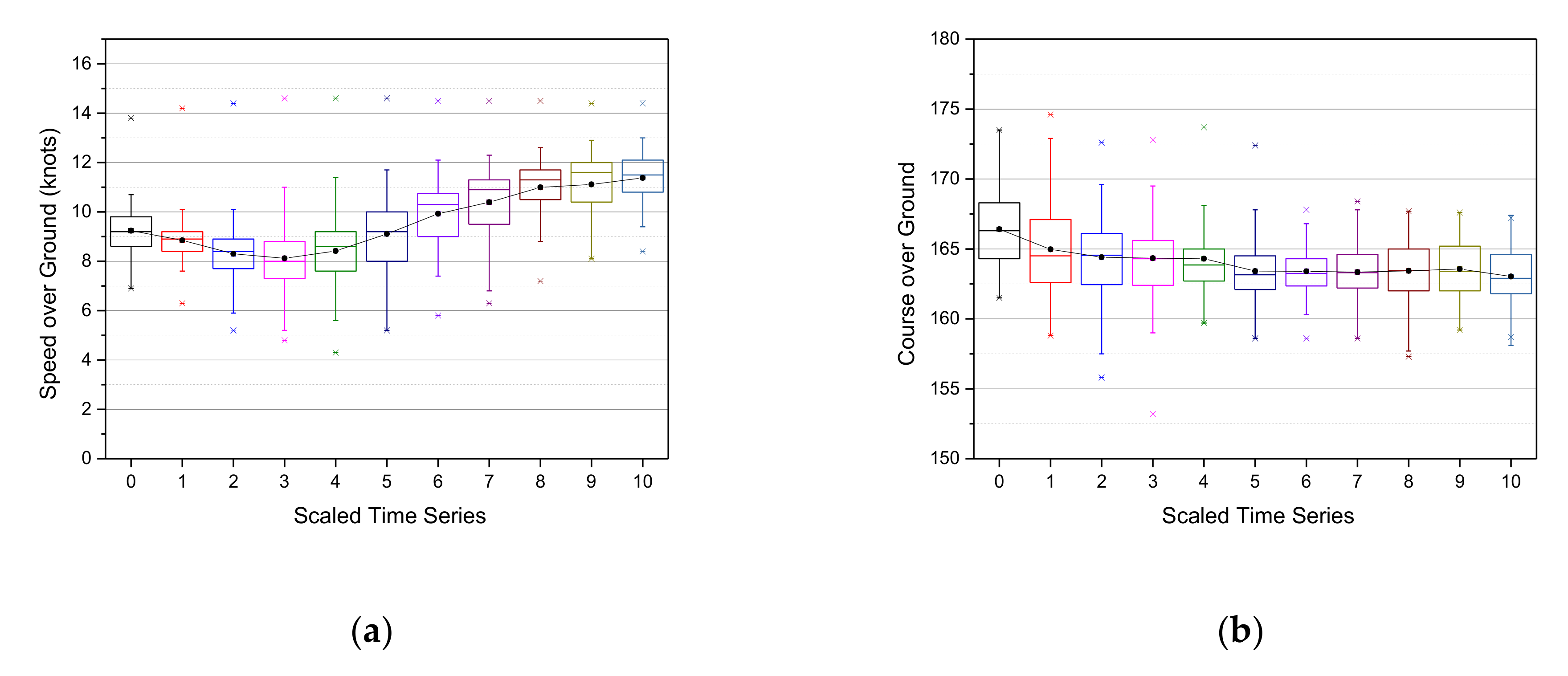
Figure 35.
Boxplot time series analysis of the departure waterway phase: (a) SOG; (b) COG; * the time series analysis for Scheme 11. stages, from 0 to 10, by multiplying the result scaled in Equation (1) by 10. In addition, the boxplot was used to visually express the descriptive statistics for 11 stages.
Figure 36.
Frequency analysis of the departure phase: (a) SOG; (b) COG.
Figure 36.
Frequency analysis of the departure phase: (a) SOG; (b) COG.
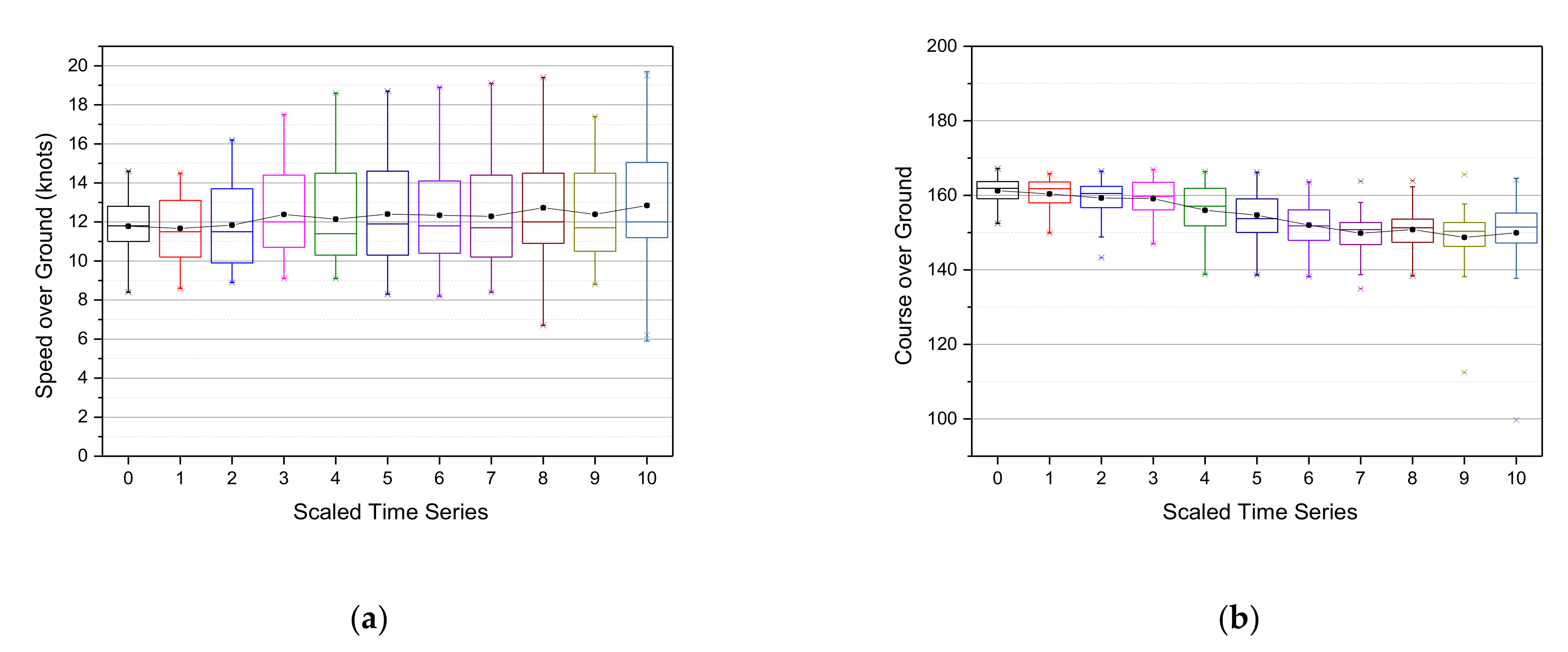
Figure 37.
Boxplot time series analysis of the departure phase: (
a) SOG; (
b) COG; * the time series analysis for ship trajec
Table 11. stages, from 0 to 10, by multiplying the result scaled in Equation (1) by 10. In addition, the boxplot was used to visually express the descriptive statistics for 11 stages.
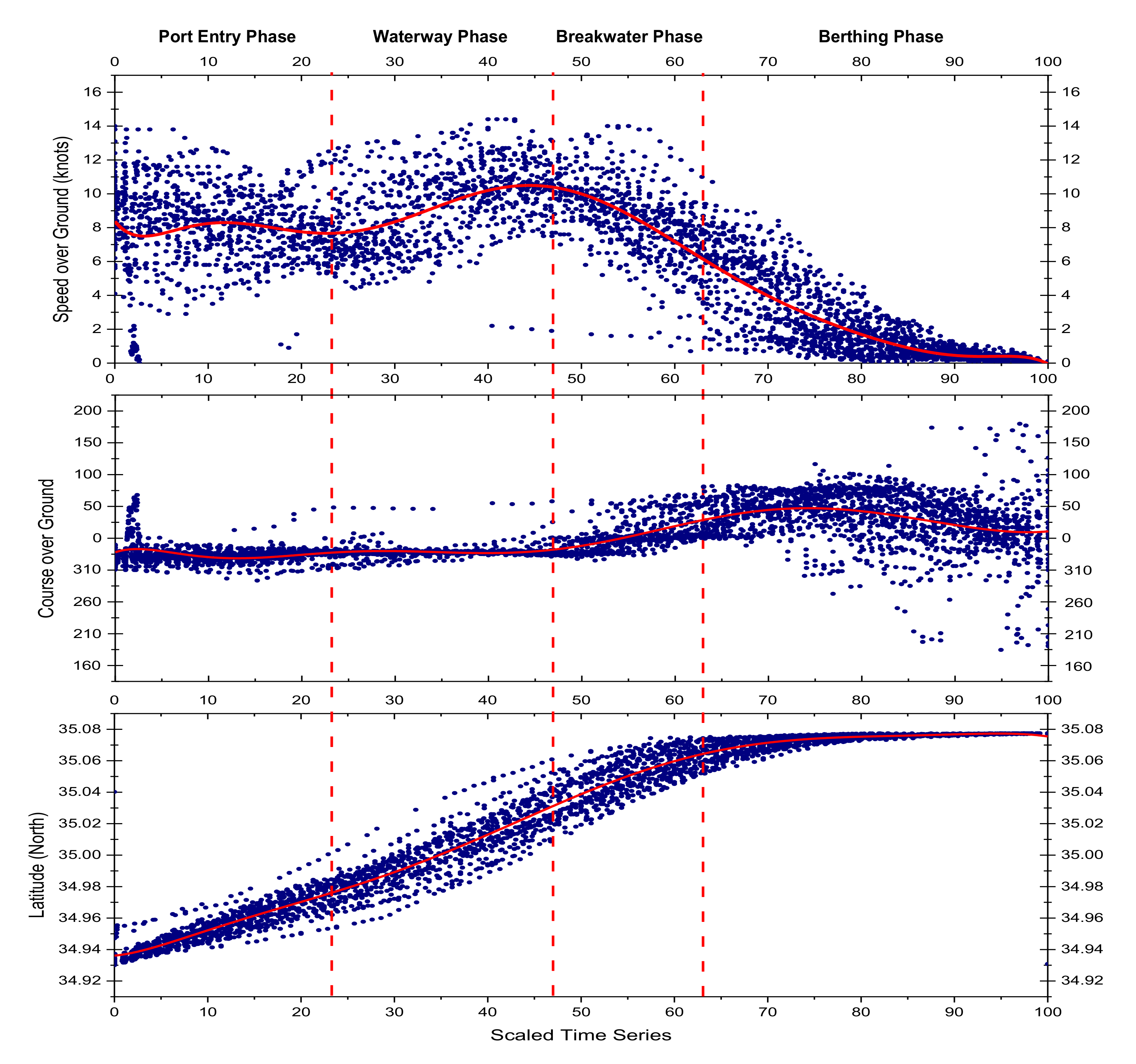
Figure 38.
Scatter graph of arriving ship trajectories for maneuvering guidelines.
Figure 38.
Scatter graph of arriving ship trajectories for maneuvering guidelines.
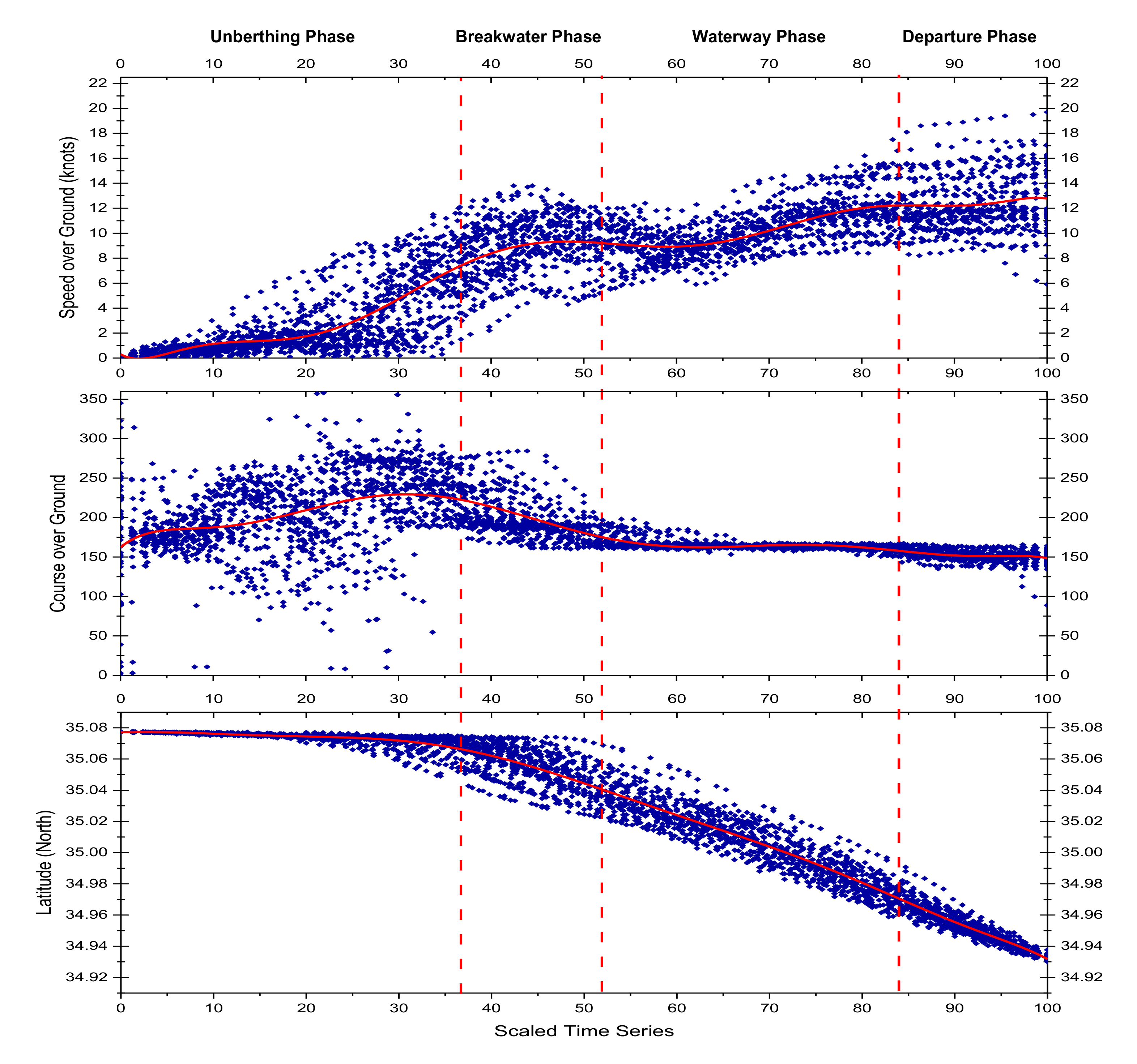
Figure 39.
Scatter graph of departing ship trajectories for maneuvering guidelines.
Figure 39.
Scatter graph of departing ship trajectories for maneuvering guidelines.
Table 1.
Characteristics of the target piers.
Table 1.
Characteristics of the target piers.
| Pier | Pier Length | Water Depth | Simultaneous Berthing Capacity |
|---|
| New Port 2 Pier | 2000 m | 16~17 m | 6 ships/4000 TEU |
| New Port 3 Pier | 1100 m | 18 m | 2 ships/4000 TEU, two ships/2000 TEU |
Table 2.
Automatic identification system (AIS) data characteristics for analysis.
Table 2.
Automatic identification system (AIS) data characteristics for analysis.
| Categorization | Automatic Identification System Data |
|---|
| Period | 01 January 2020~30 April 2020 |
| Collection Area | Latitude 034.8 N~035.1 N, Longitude 128.7 E~129.0 E |
| (Around Busan New Port) |
| Pier | Pier 2 No.4 |
| Pier 2 No.5 |
| Pier 3 No.1 |
| Ship Type | Container ship |
| Size of ship | Gross tonnage 100~220 K |
| Information | Ship’s position (latitude, longitude) |
| Speed over ground (knots) |
Course over ground (degree)
Ship’s position (latitude, longitude) |
Table 3.
Number of ships and berthings.
Table 3.
Number of ships and berthings.
| Status | Number of Ships | Number of Berthings |
|---|
| 1 Time | 2 Times | ≥3 Times | Total | Pier 2
No.4 | Pier 2
No.5 | Pier 3
No.1 | Total |
|---|
| Arrival | 36 | 5 | 1 | 42 | 28 | 21 | 1 | 50 |
| Departure | 35 | 6 | 1 | 42 | 28 | 21 | 1 | 50 |
Table 4.
Number of times and on which side ships passed Todo.
Table 4.
Number of times and on which side ships passed Todo.
| Status | Todo
Passing | Pier | Total |
|---|
| Pier 2 No.4 | Pier 2 No.5 | Pier 3 No.1 |
|---|
| Arrival | Left | 5 | 17 | 1 | 23 |
| Right | 23 | 4 | - | 27 |
| Departure | Left | 18 | 12 | 1 | 31 |
| Right | 10 | 9 | - | 19 |
Table 5.
Descriptive statistics for the port entry phase of the scaled time series.
Table 5.
Descriptive statistics for the port entry phase of the scaled time series.
| Scaled Time | Speed Over Ground | Course Over Ground |
|---|
| Mean | Std. | Min | Median | Max | Mean | Std. | Min | Median | Max |
|---|
| 0 | 9.23 | 2.41 | 4.10 | 9.55 | 14.00 | 330.03 | 10.09 | 310.60 | 329.00 | 349.80 |
| 1 | 8.41 | 2.10 | 3.50 | 8.55 | 13.00 | 326.01 | 8.83 | 309.90 | 326.60 | 346.00 |
| 2 | 8.68 | 2.28 | 2.90 | 9.00 | 13.80 | 329.54 | 10.40 | 305.09 | 330.20 | 350.50 |
| 3 | 8.41 | 2.30 | 2.90 | 8.30 | 13.80 | 325.13 | 42.28 | 0.10 | 330.40 | 349.10 |
| 4 | 8.10 | 2.23 | 3.40 | 8.40 | 12.20 | 323.95 | 40.11 | 0.80 | 328.25 | 350.80 |
| 5 | 8.05 | 2.24 | 3.80 | 8.40 | 13.80 | 330.00 | 12.03 | 296.60 | 330.90 | 354.60 |
| 6 | 8.05 | 2.17 | 4.00 | 8.20 | 12.60 | 329.04 | 11.97 | 293.50 | 330.10 | 349.10 |
| 7 | 8.08 | 2.17 | 0.90 | 8.40 | 12.40 | 328.81 | 10.73 | 306.30 | 330.25 | 350.30 |
| 8 | 8.38 | 2.13 | 1.70 | 8.60 | 13.80 | 328.38 | 8.20 | 310.10 | 329.60 | 344.60 |
| 9 | 8.31 | 1.93 | 4.40 | 8.60 | 13.30 | 331.42 | 7.52 | 312.30 | 332.50 | 344.50 |
| 10 | 8.09 | 1.63 | 4.70 | 8.20 | 12.60 | 325.95 | 48.11 | 5.80 | 334.20 | 348.90 |
| TS1 1 | 7.32 | 0.45 | 6.30 | 7.40 | 8.10 | 337.25 | 5.69 | 320.10 | 337.20 | 354.50 |
Table 6.
Descriptive statistics for the arrival waterway phase of the scaled time series.
Table 6.
Descriptive statistics for the arrival waterway phase of the scaled time series.
| Scaled Time | Speed Over Ground | Course Over Ground |
|---|
| Mean | Std. | Min | Median | Max | Mean | Std. | Min | Median | Max |
|---|
| 0 | 7.78 | 1.67 | 5.30 | 7.75 | 12.60 | 329.27 | 46.13 | 0.20 | 335.80 | 359.50 |
| 1 | 7.65 | 2.12 | 4.90 | 7.60 | 13.60 | 335.30 | 4.94 | 322.20 | 335.90 | 346.50 |
| 2 | 7.97 | 2.08 | 4.50 | 7.30 | 14.10 | 332.48 | 38.50 | 1.80 | 337.00 | 359.50 |
| 3 | 7.96 | 2.10 | 4.70 | 7.45 | 14.40 | 329.53 | 53.87 | 2.60 | 337.15 | 356.10 |
| 4 | 8.61 | 2.22 | 4.80 | 8.30 | 14.40 | 338.21 | 2.87 | 331.30 | 338.00 | 349.70 |
| 5 | 9.67 | 1.99 | 5.80 | 9.90 | 13.10 | 338.65 | 2.39 | 329.10 | 338.45 | 344.70 |
| 6 | 10.35 | 1.69 | 5.70 | 10.50 | 13.40 | 338.51 | 2.33 | 327.40 | 338.50 | 346.60 |
| 7 | 10.49 | 1.75 | 6.00 | 10.70 | 13.60 | 337.93 | 2.80 | 325.00 | 338.10 | 344.00 |
| 8 | 10.77 | 1.77 | 6.90 | 10.60 | 14.00 | 337.70 | 1.59 | 333.90 | 337.80 | 342.40 |
| 9 | 10.88 | 1.82 | 6.00 | 10.80 | 14.00 | 337.26 | 4.52 | 331.00 | 336.95 | 359.10 |
| 10 | 10.59 | 1.47 | 5.30 | 10.50 | 13.80 | 331.49 | 43.78 | 0.20 | 336.95 | 355.10 |
Table 7.
Descriptive statistics for the arrival breakwater phase of the scaled time series.
Table 7.
Descriptive statistics for the arrival breakwater phase of the scaled time series.
| Scaled Time | Speed Over Ground | Course Over Ground |
|---|
| Mean | Std. | Min | Median | Max | Mean | Std. | Min | Median | Max |
|---|
| 0 | 10.25 | 0.96 | 7.20 | 10.30 | 12.10 | 338.93 | 5.64 | 332.60 | 337.40 | 356.70 |
| 1 | 9.44 | 1.08 | 8.00 | 9.90 | 10.40 | 346.56 | 11.67 | 333.90 | 344.20 | 359.80 |
| 2 | 10.02 | 0.90 | 8.40 | 10.30 | 11.40 | 340.29 | 4.57 | 333.00 | 339.20 | 348.80 |
| 3 | 10.00 | 0.72 | 8.00 | 10.25 | 10.80 | 344.60 | 6.83 | 336.20 | 343.30 | 358.00 |
| 4 | 9.75 | 1.11 | 7.20 | 9.80 | 11.50 | 345.97 | 7.73 | 333.50 | 345.20 | 358.80 |
| 5 | 9.73 | 0.82 | 7.80 | 10.00 | 11.30 | 346.85 | 6.98 | 333.60 | 347.70 | 359.40 |
| 6 | 8.86 | 0.67 | 7.90 | 8.95 | 10.00 | 354.74 | 6.23 | 338.00 | 356.80 | 360.7 |
| 7 | 9.23 | 0.91 | 7.60 | 9.25 | 10.80 | 354.52 | 4.52 | 340.70 | 355.65 | 359.4 |
| 8 | 9.20 | 0.73 | 7.30 | 9.50 | 10.40 | 355.29 | 4.12 | 343.90 | 355.60 | 361.5 |
| 9 | 8.80 | 0.88 | 7.20 | 8.80 | 10.90 | 356.05 | 4.25 | 342.80 | 356.85 | 361.8 |
| 10 | 8.70 | 1.04 | 6.70 | 8.70 | 10.50 | 357.78 | 2.31 | 347.20 | 358.50 | 360.8 |
Table 8.
Descriptive statistics for the left-side berthing phase of the scaled time series.
Table 8.
Descriptive statistics for the left-side berthing phase of the scaled time series.
| Scaled Time | Speed Over Ground | Course Over Ground |
|---|
| Mean | Std. | Min | Median | Max | Mean | Std. | Min | Median | Max |
|---|
| TS 3_1 | 8.02 | 0.69 | 6.50 | 8.20 | 9.20 | 2.49 | 2.45 | −1.00 | 1.80 | 11.00 |
| TS 3_2 | 7.58 | 0.52 | 6.30 | 7.60 | 8.30 | 4.79 | 2.67 | 1.10 | 5.10 | 11.10 |
| TS 3_3 | 7.02 | 0.57 | 6.10 | 7.00 | 8.10 | 11.01 | 8.45 | 0.20 | 9.40 | 29.10 |
| Leg 3_1 | 6.38 | 1.67 | 4.90 | 6.00 | 12.20 | 21.24 | 19.61 | −5.90 | 16.30 | 65.60 |
| Leg 3_2 | 5.44 | 1.01 | 4.40 | 5.30 | 10.70 | 33.80 | 24.96 | 0.00 | 28.50 | 75.90 |
| Leg 3_3 | 4.88 | 0.91 | 3.50 | 4.80 | 8.90 | 47.27 | 22.33 | 10.50 | 50.10 | 78.30 |
| Leg 3_4 | 4.10 | 0.51 | 2.90 | 4.10 | 5.20 | 61.99 | 12.13 | 31.70 | 62.40 | 84.50 |
| Berth 1 | 2.33 | 0.72 | 0.40 | 2.30 | 3.80 | 72.64 | 9.45 | 26.90 | 72.60 | 101.10 |
| Berth 2 | 0.95 | 0.55 | 0.00 | 0.80 | 2.40 | 54.36 | 26.52 | −17.30 | 60.10 | 101.40 |
| Berth 3 | 0.27 | 0.23 | 0.00 | 0.20 | 1.10 | 20.42 | 49.23 | −175.50 | 21.80 | 179.80 |
Table 9.
Descriptive statistics for the right-side berthing phase of the scaled time series.
Table 9.
Descriptive statistics for the right-side berthing phase of the scaled time series.
| Scaled Time | Speed Over Ground | Course Over Ground |
|---|
| Mean | Std. | Min | Median | Max | Mean | Std. | Min | Median | Max |
|---|
| TS 3_1 | 8.42 | 0.81 | 6.90 | 8.40 | 11.10 | 4.99 | 6.12 | 0.00 | 3.20 | 32.40 |
| TS 3_2 | 7.94 | 0.90 | 6.50 | 7.80 | 10.60 | 10.81 | 8.10 | 0.10 | 10.90 | 26.50 |
| TS 3_3 | 7.65 | 0.87 | 6.20 | 7.40 | 10.20 | 24.01 | 10.16 | 4.20 | 23.20 | 42.20 |
| Leg 3_1 | 6.80 | 1.25 | 4.00 | 6.50 | 10.10 | 40.67 | 16.62 | 0.10 | 44.00 | 73.80 |
| Leg 3_2 | 5.97 | 1.79 | 1.20 | 5.80 | 9.40 | 51.45 | 11.30 | 19.30 | 51.20 | 79.10 |
| Leg 3_3 | 4.96 | 2.10 | 0.50 | 5.10 | 7.90 | 44.23 | 32.18 | −87.40 | 50.75 | 78.10 |
| Leg 3_4 | 4.06 | 1.44 | 1.20 | 4.10 | 7.10 | 32.30 | 37.44 | −49.90 | 47.10 | 69.80 |
| Berth 1 | 1.61 | 0.79 | 0.20 | 1.50 | 3.40 | 25.24 | 33.11 | −74.90 | 34.50 | 116.40 |
| Berth 2 | 0.80 | 0.41 | 0.00 | 0.80 | 2.20 | 16.10 | 39.53 | −162.90 | 22.90 | 74.90 |
| Berth 3 | 0.32 | 0.24 | 0.00 | 0.20 | 1.30 | 12.44 | 51.53 | −168.70 | 11.25 | 173.70 |
Table 10.
Descriptive statistics for left-side unberthing phase of the scaled time series.
Table 10.
Descriptive statistics for left-side unberthing phase of the scaled time series.
| Scaled Time | Speed Over Ground | Course Over Ground |
|---|
| Mean | Std. | Min | Median | Max | Mean | Std. | Min | Median | Max |
|---|
| TS 3_1 | 0.24 | 0.25 | 0.00 | 0.20 | 1.00 | 178.92 | 48.49 | 0.00 | 177.30 | 345.00 |
| TS 3_2 | 0.74 | 0.44 | 0.10 | 0.70 | 3.00 | 200.06 | 30.32 | 110.80 | 192.30 | 259.50 |
| TS 3_3 | 1.04 | 0.54 | 0.10 | 1.10 | 2.60 | 196.78 | 27.03 | 125.60 | 192.40 | 277.50 |
| Leg 3_1 | 1.38 | 0.88 | 0.40 | 1.15 | 5.80 | 224.21 | 53.54 | 8.90 | 229.85 | 357.00 |
| Leg 3_2 | 2.62 | 1.61 | 0.10 | 2.30 | 6.70 | 239.37 | 61.14 | 9.80 | 263.85 | 358.10 |
| Leg 3_3 | 4.94 | 1.57 | 0.80 | 5.10 | 8.30 | 258.06 | 22.67 | 199.30 | 261.90 | 327.80 |
| Leg 3_4 | 7.09 | 1.07 | 5.00 | 7.00 | 10.40 | 211.20 | 19.19 | 185.10 | 203.60 | 258.60 |
| Berth 1 | 8.92 | 0.91 | 7.50 | 8.80 | 12.70 | 190.60 | 3.47 | 181.00 | 190.60 | 200.90 |
| Berth 2 | 10.22 | 0.97 | 8.40 | 10.50 | 11.80 | 188.61 | 2.60 | 184.00 | 189.50 | 193.40 |
| Berth 3 | 10.67 | 1.04 | 8.40 | 10.90 | 12.10 | 187.50 | 3.84 | 179.90 | 187.95 | 197.90 |
Table 11.
Descriptive statistics for the right-side unberthing phase of the scaled time series.
Table 11.
Descriptive statistics for the right-side unberthing phase of the scaled time series.
| Scaled Time | Speed Over Ground | Course Over Ground |
|---|
| Mean | Std. | Min | Median | Max | Mean | Std. | Min | Median | Max |
|---|
| TS 3_1 | 0.31 | 0.30 | 0.00 | 0.20 | 1.10 | 166.82 | 60.43 | 0.00 | 174.50 | 322.70 |
| TS 3_2 | 0.70 | 0.39 | 0.00 | 0.70 | 2.00 | 169.89 | 32.69 | 10.60 | 173.20 | 224.60 |
| TS 3_3 | 1.18 | 0.89 | 0.00 | 0.90 | 4.20 | 160.96 | 31.93 | 10.60 | 169.80 | 241.70 |
| Leg 3_1 | 1.97 | 1.31 | 0.10 | 1.70 | 6.20 | 187.98 | 54.59 | 83.40 | 207.30 | 298.20 |
| Leg 3_2 | 3.68 | 2.27 | 0.20 | 2.95 | 9.60 | 204.77 | 45.60 | 69.20 | 226.95 | 324.50 |
| Leg 3_3 | 7.45 | 2.39 | 1.20 | 7.80 | 12.60 | 233.12 | 12.78 | 157.50 | 235.85 | 248.10 |
| Leg 3_4 | 9.60 | 2.07 | 1.70 | 9.75 | 13.20 | 209.32 | 10.81 | 175.30 | 207.30 | 243.10 |
| Berth 1 | 9.31 | 1.65 | 6.00 | 9.70 | 11.80 | 196.52 | 9.41 | 188.30 | 192.30 | 223.30 |
| Berth 2 | 10.35 | 1.94 | 6.50 | 10.70 | 13.10 | 195.47 | 14.27 | 171.30 | 194.60 | 232.20 |
| Berth 3 | 10.34 | 2.03 | 6.70 | 10.45 | 13.80 | 190.86 | 9.48 | 171.30 | 191.70 | 205.60 |
Table 12.
Descriptive statistics for the departure breakwater phase of the scaled time series.
Table 12.
Descriptive statistics for the departure breakwater phase of the scaled time series.
| Scaled Time | Speed Over Ground | Course Over Ground |
|---|
| Mean | Std. | Min | Median | Max | Mean | Std. | Min | Median | Max |
|---|
| 0 | 10.47 | 1.33 | 7.60 | 10.55 | 13.20 | 183.06 | 7.79 | 167.70 | 182.15 | 200.20 |
| 1 | 11.57 | 1.85 | 8.30 | 12.25 | 13.80 | 184.66 | 6.15 | 173.00 | 188.05 | 190.00 |
| 2 | 10.53 | 1.35 | 7.60 | 10.60 | 13.50 | 177.08 | 9.10 | 163.00 | 177.10 | 197.00 |
| 3 | 10.82 | 1.49 | 7.70 | 11.05 | 13.10 | 177.28 | 7.98 | 162.00 | 178.35 | 192.70 |
| 4 | 10.77 | 0.67 | 9.60 | 10.80 | 11.70 | 171.91 | 9.96 | 162.00 | 167.35 | 189.70 |
| 5 | 9.77 | 1.18 | 7.30 | 10.00 | 13.40 | 170.47 | 5.71 | 161.30 | 169.45 | 183.80 |
Table 13.
Descriptive statistics for the departure waterway phase of the scaled time series.
Table 13.
Descriptive statistics for the departure waterway phase of the scaled time series.
| Scaled Time | Speed Over Ground | Course Over Ground |
|---|
| Mean | Std. | Min | Median | Max | Mean | Std. | Min | Median | Max |
|---|
| 0 | 9.24 | 1.07 | 6.90 | 9.20 | 13.80 | 166.41 | 3.04 | 161.50 | 166.30 | 173.50 |
| 1 | 8.85 | 1.39 | 6.30 | 8.90 | 14.20 | 164.97 | 3.26 | 158.80 | 164.50 | 174.60 |
| 2 | 8.30 | 1.21 | 5.20 | 8.40 | 14.40 | 164.41 | 2.94 | 155.80 | 164.55 | 172.60 |
| 3 | 8.12 | 1.54 | 4.80 | 8.00 | 14.60 | 164.33 | 3.12 | 153.20 | 164.30 | 172.80 |
| 4 | 8.42 | 1.49 | 4.30 | 8.60 | 14.60 | 164.30 | 2.58 | 159.70 | 163.85 | 173.70 |
| 5 | 9.11 | 1.70 | 5.20 | 9.20 | 14.60 | 163.42 | 2.35 | 158.60 | 163.15 | 172.40 |
| 6 | 9.93 | 1.60 | 5.80 | 10.30 | 14.50 | 163.40 | 1.80 | 158.60 | 163.25 | 167.80 |
| 7 | 10.39 | 1.44 | 6.30 | 10.90 | 14.50 | 163.34 | 1.98 | 158.60 | 163.30 | 168.40 |
| 8 | 10.99 | 1.44 | 7.20 | 11.30 | 14.50 | 163.43 | 2.10 | 157.30 | 164.60 | 167.70 |
| 9 | 11.11 | 1.34 | 8.10 | 11.60 | 14.40 | 163.56 | 2.11 | 159.20 | 165.20 | 167.60 |
| 10 | 11.38 | 1.12 | 8.40 | 11.50 | 14.50 | 163.03 | 2.02 | 158.10 | 164.60 | 167.40 |
Table 14.
Descriptive statistics for the departure phase of the scaled time series.
Table 14.
Descriptive statistics for the departure phase of the scaled time series.
| Scaled Time | Speed Over Ground | Course Over Ground |
|---|
| Mean | Std. | Min | Median | Max | Mean | Std. | Min | Median | Max |
|---|
| 0 | 11.78 | 1.36 | 8.40 | 11.80 | 14.60 | 161.23 | 3.43 | 152.50 | 161.90 | 167.20 |
| 1 | 11.67 | 1.59 | 8.60 | 11.50 | 14.50 | 160.38 | 4.49 | 149.90 | 161.80 | 165.80 |
| 2 | 11.84 | 1.95 | 8.90 | 11.50 | 16.20 | 159.29 | 4.79 | 143.30 | 160.50 | 166.50 |
| 3 | 12.39 | 2.19 | 9.10 | 12.00 | 17.50 | 159.11 | 4.97 | 147.00 | 159.70 | 166.90 |
| 4 | 12.14 | 2.28 | 9.10 | 11.40 | 18.60 | 156.00 | 6.10 | 138.80 | 157.10 | 166.40 |
| 5 | 12.40 | 2.40 | 8.30 | 11.90 | 18.70 | 154.69 | 6.09 | 138.60 | 153.75 | 166.20 |
| 6 | 12.34 | 2.29 | 8.20 | 11.80 | 18.90 | 151.99 | 5.61 | 138.20 | 151.80 | 163.60 |
| 7 | 12.29 | 2.47 | 8.40 | 11.70 | 19.10 | 149.86 | 6.34 | 134.90 | 150.80 | 163.80 |
| 8 | 12.73 | 2.62 | 6.70 | 12.00 | 19.40 | 150.80 | 3.13 | 138.40 | 151.30 | 163.90 |
| 9 | 12.39 | 2.53 | 8.80 | 11.70 | 17.40 | 148.71 | 8.40 | 112.50 | 150.35 | 165.60 |
| 10 | 12.84 | 2.60 | 5.90 | 12.00 | 19.70 | 149.93 | 9.76 | 88.70 | 151.50 | 164.60 |
Table 15.
R-square analysis result of the fitting line.
Table 15.
R-square analysis result of the fitting line.
| Guideline Items | R-Squared Values of the Fitting Line |
|---|
| Arrival | Departure |
|---|
| Speed over ground | 0.7788 | 0.8414 |
| Course over ground | 0.4564 | 0.4186 |
| Ship’s position (latitude) | 0.9756 | 0.9800 |


