Flatness-Based Aggressive Formation Tracking Control of Quadrotors with Finite-Time Estimated Feedforwards

Abstract

In this paper we address a decentralized neighbor-based formation tracking control of multiple quadrotors with leader–follower structure. Different from most of the existing work, the formation tracking controller is given in one loop without distinguishing the motion control and attitude control by means of the theory of flatness. In order to achieve an aggressive formation tracking, the high-order states of the neighbors motion are estimated by using a proposed extended finite-time observer for each quadrotor. Then the estimated motion states are used as feedforwards in the formation controller design. Simulation and experimental results show that the proposed formation controller improves the formation performance, i.e., the formation pattern of the quadrotors is better maintained than that using the formation controller without high-order feedforwards, when tracking an aggressive reference formation trajectory.

1. Introduction

The cooperative control of multi-quadrotor systems has progressively attracted attention of researchers in both civil and military areas [1]. Especially, in the application of object transportation, the formation of multiple quadrotors has potential application significance [2,3,4,5,6].

The formation control problem can be categorized into two types. Namely, the formation producing problem and the formation tracking problem [7]. The former problem refers to the algorithm design for a group of vehicles to reach a predefined geometric pattern without a group reference [8,9,10], while the latter problem refers to the same task and meanwhile following a predefined trajectory [11,12,13]. The object transformation is a typical formation tracking problem, which is considered in this paper. An external reference formation trajectory (RFT) is given to the leading quadrotor(s) to guide the formation. We note that in the case of multiple leaders, they share the same RFT. According to [14,15], the formation tracking problem can be attributed as a consensus problem.

In most aggressive maneuver cases, the quadrotor is controlled in tracking a desired aggressive moving trajectory that is prescribed a prior, for instance, by polynomials w.r.t time. A widely used method is the control of geometry on Lie group ($SE(3)$ for example). The aggressive formation problem of multiple quadrotors is investigated in [16], where the quadrotors are permitted to move quickly in 3-D environment with a tight formation. The formation of quadrotors is based on proper trajectory generation process, thereby, the full information of the trajectory (including each order derivatives) are known. However, in a multi-agent system with neighbor-based decentralized control, it is impossible to enforce the motion of quadrotor by generating polynomials-based trajectories.

The flatness-based control is frequently used in the trajectory planing for high-order dynamical system. For instance, the time-optimal trajectory generation problem is investigated for helicopter landing in [17] and for multi-rotor in [18]. Especially, in [18], the trajectory is planned in real-time. The agile maneuvers for a quadrotor with a cable-suspended load are investigated in [19]. In this work, by means of flatness-based planning, the air vehicle is able to behave in aggressive maneuver, real-time collision avoidance, and time optimal flight. However, the planned trajectory’s high-order derivatives are required for the quadrotor. In the decentralized formation tracking control of quadrotors, each quadrotor (including the leader) has to behave according to the state of neighbors, which are in general not able or difficult to get the full information of these states.

In multi-agent systems, the consensus speed of agents with linear dynamics depends on the minimum non-singular eigenvalue of the interaction matrix (or Laplacian) [20] and the absolute value of the maximum pole in left half plane of agent dynamics [21]. For the formation of quadrotors, the idea in this paper is to propose a nonlinear formation controller, in order to use these existing results.

One of the difficulties in the control of multi-quadrotor systems is that the quadrotor has under-actuated, nonlinear, and coupling dynamics. The existing consensus algorithms in the literature, which are mostly developed for single-integrator or double-integrator agent dynamics, have not satisfactory formation performance for the formation control of quadrotors in practice, especially in aggressive formation tracking where the small angle assumption should be removed. Furthermore, lacking velocities and its higher derivatives of the neighbors’ states and the RFT makes aggressive formation non-trivial. Nevertheless, in very recent years, the researchers start to consider the nonlinearities/disturbances in formation control [1,22].

In this paper, we aimed at proposing an aggressive control framework for a class of systems with high-order dynamics (in special, quadrotor). Instead of using inner-outer loop structure, we directly design the torques by using the flatness theory, where the high-order cooperative errors are used. The formation controller is decentralized, since the quadrotors move based on the measurement to their neighbors (in special, positions. We suppose that the velocities and higher-order derivatives are not available). Then, the main contributions of this paper are three-fold. A flatness-based formation control with estimated feedforwards is proposed such that the aggressive formation is attained. In order to estimate the velocities and higher-order derivatives of the neighbors states, an extended finite-time observer is proposed. To avoid probably instability caused by the great initial deviation of the estimated states, the saturated feedforwards are developed to improve the formation controller, the convergence of the formation tracking error is then analyzed.

We note that our proposed controller can be combined with the existing methods by adding some nonlinear compositions into the controller, for instance, to deal with the bounded nonlinearities (uncertainties), to achieve asymptotic convergence, to improve the formation speed. These methods can be listed such as robust compensation [20,22], composite nonlinear feedback [13], artificial neural network estimation [23].

The paper is organized as follows. Some preliminaries in graph theory are given in Section 2. The aggressive control of quadrotors with finite-time observer is presented in Section 3. The formation control design and the stability analysis are shown in Section 4. Some simulation and experimental results are given in Section 5. Finally, some conclusions are stated in Section 6. Some useful notations and definitions are given as follows.

Notations: The real vectorial field is represented by ${\mathbb{R}}^m$. Notation ${\mathbb{R}}^{+}$ represents real positive numbers. The saturation function ${\sigma }_b:{\mathbb{R}}^n\to {\mathbb{R}}^n$ is defined as follows, if $n=1$, ${\sigma }_b(a)=\begin{array}{c}\mathrm{sign}(a)·min\{\parallel a\parallel ,b\}\end{array}$, where $\mathrm{sign}(·)$ represents the sign function. If $n>1$ and $a={[a_1,\cdots ,a_n]}^T$, then, ${\sigma }_b(a)={[{\sigma }_b(a_1),\cdots ,{\sigma }_b(a_n)]}^T$. In special, if $b=\infty$, the saturation function is equal to a linear function without saturation, i.e., ${\sigma }_{\infty }(a)=a$, for any $a\in \mathbb{R}$. The notation $C^m(\mathbb{R},{\mathbb{R}}^n)$ represents the ensemble of $m-$order continuous manifolds in $\mathbb{R}\to {\mathbb{R}}^n$. The notations $I_n$ and ${\mathbf{0}}_{n\times n}$ represent identical and zero matrices in ${\mathbb{R}}^{n\times n}$. In special, ${\mathbf{1}}_n$ and ${\mathbf{0}}_n$ represent the vectors with all entries equal to one and zero in ${\mathbb{R}}^n$, respectively. Function ${\lambda }_i(·)$ represents the i-th eigenvalue of matrix inside the parenthesis, in special, ${\lambda }_{max}(·)$ and ${\lambda }_{min}(·)$ represent the maximum and minimum eigenvalue of matrix inside the parenthesis, respectively.

2. Preliminaries

Some basic knowledge in graph theory and ‘interaction matrix’ is given in this section. Some propositions and corollaries about the interaction matrix are introduced, which are useful in the analysis of the consensus of quadrotors in Section 4.

2.1. Graph Theory

Graph theory is helpful to represent the interaction relations of multi-agent systems. A graph $\mathcal{G}=(\mathcal{V},\mathcal{E})$ is normally with the sets of vertices $\mathcal{V}$ and edges $\mathcal{E}$. The set of vertices $\mathcal{V}=\left\{1,2,\dots ,n\right\}$ is composed of the indices of agents. $\left|\mathcal{V}\right|$ represents the cardinality of the set $\mathcal{V}$, which satisfies $\left|\mathcal{V}\right|=n$. The set of edges is represented by $\mathcal{E}\subseteq \mathcal{V}\times \mathcal{V}$. If an edge exists between two vertices, the two vertices are called adjacent. In this work, simple and undirected graphs are considered.

The adjacency matrix of $\mathcal{G}$ is denoted by $G^A=\left[a_{ij}\right]\in R^{n\times n}$, where $a_{ij}$ represents the connection of nodes i and j on a graph. Since the simple graph is considered, we have $a_{ii}=0$. Since the graph is undirected, we have $a_{ij}=a_{ji}$ and $a_{ij}=1$ if $(i,j)\in \mathcal{E}$, otherwise, $a_{ij}=0$. The degree matrix of $\mathcal{G}$ is denoted by $G^D=\mathrm{diag}\{{\sum }_{j=1}^n{a}_{1j},\cdots ,{\sum }_{j=1}^n{a}_{nj}\}$. The neighbor set ${\mathcal{N}}_i=\{j\in \mathcal{V}:(i,j)\in \mathcal{E}\}$ of agent i, is composed of the indices of the agents j, which has interaction with the agent i. In other words, if $a_{ij}>0$, then, agent j is a neighbor of agent i. The number of neighbors of agent i is equal to $|{\mathcal{N}}_i|$.

We define a diagonal matrix $G^L=\mathrm{diag}\{l_1,\cdots ,l_n\}$, which indicates the knowledge of reference formation trajectory (RFT) of each agent. If $l_i=1$, agent i can obtain the RFT (by sensing/detecting), i.e., a leader. Otherwise, if $l_i=0$, agent i is a follower, for $i\in \mathcal{V}$. Then, the leader set is defined as ${\mathcal{V}}_L=\{i\in \mathcal{V}:l_i>0\}$. The leader set ${\mathcal{V}}_L\subset \mathcal{V}$ is a subset of $\mathcal{V}$, which contains the indices of the leaders. Particularly, all the quadrotors are leaders, when ${\mathcal{V}}_L=\mathcal{V}$. The indices of the followers are contained in the complementary set of ${\mathcal{V}}_L$, namely, $\mathcal{V}-{\mathcal{V}}_L$.

2.2. Interaction Matrix

We propose an interaction matrix G for representing the interconnecting relations of quadrotors with leader–follower (L–F) configuration as follows.

$$G=G^D-G^A+G^L$$

(1)

Remark 1.

Let us note that the first two terms $G^D-G^A$ are normally called the Laplacian in graph theory.

Proposition 1.

Let $\mathcal{G}$ be an undirected simple graph, then the interconnection matrix G in Equation (1), is positive-definite, if (i) $\mathcal{G}$ is connected; (ii) ${\mathcal{V}}_L\ne \mathrm{\Phi }$, where Φ represents a null set.

Proof. 

Since $\mathcal{G}$ is connected, we have $G^D-G^A\ge 0$. Considering the definition of $G^L$, we have $G^L\ge 0$. We prove this proposition by contradiction. Firstly, we suppose that there exists a nonzero vector $x\in {\mathbb{R}}^n$, which renders

$$x^{T}Gx=x^T(L+G^L)x=x^{T}Lx+x^T{G}^{L}x=0$$

Therefore, we must have $x^{T}Lx=0$ and $x^T{G}^{L}x=0$.

Since $x^{T}Lx=0$, we obtain that $x=\alpha {\mathbf{1}}_n$, where $\alpha$ is a nonzero scalar. According to the fact that ${\mathcal{V}}_L\ne \mathrm{\Phi }$, then, $G^L\ne 0$. As a result, $x^T{G}^{L}x={\alpha }^2{\mathbf{1}}_n^T{G}^L{\mathbf{1}}_n>0$, which contradicts $x^T{G}^{L}x=0$. Therefore, such a nonzero vector x does not exist. Thus, for any nonzero vector x, $x^{T}Gx>0$, namely, G is positive-definite. □

When condition (i) is not satisfied such that $\mathcal{G}$ is not connected, the graph can be divided into s connected sub-graphs ${\mathcal{G}}_1,{\mathcal{G}}_2,\cdots ,{\mathcal{G}}_s$. In that case, according to Proposition 1, we have the following corollary.

Corollary 1.

The interaction matrix G is positive-definite, if the leaders set satisfies ${\mathcal{V}}_L\ge s$, and ${\mathcal{V}}_{iL}\ne \mathrm{\Phi }$, where $i=\{1,2,\cdots ,s\}$.

Proof. 

If a multi-agent system contains s connected sub-groups of agents, then, the interaction matrix is block diagonal, which has s blocks on the diagonal. Since each sub-group ${\mathcal{G}}_i$, $i=\{1,2,\cdots ,s\}$ is connected and $V_{iL}\ne \mathrm{\Phi }$, then, the block in the interaction matrix is positive definite. Hence, the interaction matrix is positive definite. □

The normalized interaction matrix is defined by

$$\overline{G}={(G^D+G^L)}^{-1}G$$

(2)

The normalized interaction matrix $\overline{G}$ is not symmetric, but it has the following property.

Proposition 2.

The normalized interaction matrix $\overline{G}$ has real eigenvalues, if $\mathcal{G}$ is undirected.

Proof. 

Since $\overline{G}$ is a normalized interaction matrix, then, $\overline{G}={(G^D+G^L)}^{-1}·G$. We recall that G is symmetric.

Using ${(G^D+G^L)}^{-\frac{1}{2}}$, we apply similarity transformation to $\overline{G}$, then, we obtain that ${(G^D+G^L)}^{\frac{1}{2}}·\overline{G}·{(G^D+G^L)}^{-\frac{1}{2}}={(G^D+G^L)}^{-\frac{1}{2}}·G·{(G^D+G^L)}^{-\frac{1}{2}}$ is symmetric, because $G^D+G^L$ are diagonal and G is symmetric.

Since $\overline{G}$ is similar to ${(G^D+G^L)}^{-\frac{1}{2}}·G·{(G^D+G^L)}^{-\frac{1}{2}}$, the eigenvalues of $\overline{G}$ are real, moreover, they are equal to the eigenvalues of ${(G^D+G^L)}^{-\frac{1}{2}}·G·{(G^D+G^L)}^{-\frac{1}{2}}$. □

Corollary 2.

The normalized interaction matrix $\overline{G}$ is positive-definite, if conditions in Proposition 1 or Corollary 1 are satisfied.

Proof. 

According to the conditions in Proposition 1 or Corollary 1, we know that G is invertible. Since $\overline{G}$ is similar to ${(G^D+G^L)}^{-\frac{1}{2}}·G·{(G^D+G^L)}^{-\frac{1}{2}}$ according to Proposition 2, we obtain that $\overline{G}$ is also positive-definite. □

3. Aggressive Control of Quadrotors with Extended Finite-Time Observer

3.1. Quadrotor Model

The dynamics of a quadrotor is modelled as the motion of a rigid body in 3-D space under a thrust force and three moments, which are generated by the thrust forces of the four rotors. The notations used in the quadrotor’s model are shown in Table 1. The orientation of the quadrotor with respect to the inertial frame is represented by the rotation matrix $R_i\in \mathrm{SO}(3)$, where SO(3) represents a special orthogonal group, and whose determinant is one. Note that $R_i^T{R}_i=I$, where I represents an identical matrix. The dynamics of a quadrotor i is shown as follows

$$\left\{\begin{array}{c}m{\ddot{\mathcal{X}}}_i=-mg{\mathbf{e}}_3+R_i{F}_{T_i}{\mathbf{e}}_3\\ {\dot{R}}_i=R_{i}S({\mathrm{\Omega }}_i)\\ J{\dot{\mathrm{\Omega }}}_i+S({\mathrm{\Omega }}_i)J{\mathrm{\Omega }}_i={\tau }_i\end{array}\right.$$

(3)

where ${\mathcal{X}}_i={[X_i,Y_i,Z_i]}^T$ represents the coordinates of the center of mass of a quadrotor in the fixed inertial frame $x_e{y}_e{z}_e$. The Euler angles (pitch, roll, and yaw) are represented by the vector ${\mathrm{\Theta }}_i={[{\varphi }_i,{\theta }_i,{\psi }_i]}^T$. The first equation of (3) represents the translational dynamics in the inertial frame, where m represents the mass of a quadrotor and g represents the gravity. The rotation matrix $R_i$ in the second equation of (3) can transform the coordinates of a point from the body-fixed frame to the inertial frame. The third equation of (3) represents the rotational dynamics of quadrotor i. The inertia matrix J of a quadrotor i is represented in the body-fixed frame, according to the assumptions on the physical structure of a quadrotor, we can obtain that $J=\mathrm{diag}\{I_{x_b},I_{y_b},I_{z_b}\}$ is diagonal, where scalars $I_{x_b}$, $I_{y_b}$ and $I_{z_b}$ represent the moments of inertia with respect to $x_b$, $y_b$ and $z_b$ respectively. Additionally, we assume that all the quadrotors in the flock have the same physical coefficients such as the mass and the inertia matrix. The angular velocity of the quadrotor i in the body-fixed frame is represented by ${\mathrm{\Omega }}_i\in {\mathbb{R}}^3$. The function $S(·):{\mathbb{R}}^3\to {\mathbb{R}}^{3\times 3}$ represents an operation that transforms a vector in ${\mathbb{R}}^3$ to a skew-symmetric matrix ${\mathbb{R}}^{3\times 3}$. Given two arbitrary vectors $v_1$, $v_2\in {\mathbb{R}}^3$, the function $S(·)$ satisfies the property $S(v_1)·v_2=v_1\times v_2$. Then, according to the definition of cross product and the operation $S(·)$, we conclude that $S({\mathrm{\Omega }}_i)\in {\mathbb{R}}^{3\times 3}$ is skew-symmetric matrix in terms of the members of ${\mathrm{\Omega }}_i={[p_i,q_i,r_i]}^T$ as follows

$$S({\mathrm{\Omega }}_i)=\left[\begin{array}{ccc}0& -r_i& q_i\\ r_i& 0& -p_i\\ -q_i& p_i& 0\end{array}\right]$$

(4)

where $p_i$, $q_i$ and $r_i$ represent the angular velocities with respect to the body-fixed frame of the quadrotor i.

Table 1. The denotations of the variables in the dynamic model of quadrotor.

Symbol	Description
$x_e{y}_e{z}_e$	Fixed inertial frame
${\mathbf{e}}_1,{\mathbf{e}}_2,{\mathbf{e}}_3$	Basis vector of inertial frame ${\mathbf{e}}_1={[1,0,0]}^T$, ${\mathbf{e}}_2={[0,1,0]}^T$, ${\mathbf{e}}_3={[0,0,1]}^T$
${\mathcal{X}}_i={[X_i,Y_i,Z_i]}^T$	Coordinates of the center of mass of a quadrotor in $x_e{y}_e{z}_e$
${\mathrm{\Theta }}_i={[{\varphi }_i,{\theta }_i,{\psi }_i]}^T$	Euler angles (pitch, roll and yaw)
$R_z({\psi }_i),R_y({\theta }_i),R_x({\varphi }_i)$	Rotation matrices in yaw, pitch and roll
$R_i$	Rotation matrix $R_i=R_z({\psi }_i)R_y({\theta }_i)R_x({\varphi }_i)$
$J=\mathrm{diag}\{I_{x_b},I_{y_b},I_{z_b}\}$	Inertia matrix represented in the body-fixed frame $x_b{y}_b{z}_b$
${\mathrm{\Omega }}_i={[p_i,q_i,r_i]}^T$	Angular velocity of the quadrotor i in the body-fixed frame
$S(·):{\mathbb{R}}^3\to {\mathbb{R}}^{3\times 3}$	Operation from vector in ${\mathbb{R}}^3$ to skew-symmetric matrix ${\mathbb{R}}^{3\times 3}$
${\tau }_i={[{\tau }_{{\varphi }_i},{\tau }_{{\theta }_i},{\tau }_{{\psi }_i}]}^T\in {\mathbb{R}}^3$	The moments of roll, pitch and yaw
$F_{T_i}$	Total thrust force of quadrotor i
${\varkappa }_i=[{\mathcal{X}}_i^T,{\dot{\mathcal{X}}}_i^T]$	State of quadrotor i
$u_i={[F_{T_i},{\tau }_i^T]}^T\in {\mathbb{R}}^4$	Control input of the quadrotor i

We refer to ${\varphi }_i,{\theta }_i,{\psi }_i$ as the roll, pitch, and yaw angles, ${\tau }_i={[{\tau }_{{\varphi }_i},{\tau }_{{\theta }_i},{\tau }_{{\psi }_i}]}^T\in {\mathbb{R}}^3$ represents the roll, pitch, and yaw moments. The thrust force is represented by $F_{T_i}$. We note that ${\mathbf{e}}_3={[0,0,1]}^T$ is a constant vector. The attitude dynamics of each quadrotor is generated by moments ${\tau }_{{\varphi }_i},{\tau }_{{\theta }_i}$ and ${\tau }_{{\psi }_i}$ and thrust force $F_{T_i}$.

The rotation matrix $R_i$ from the body-fixed frame to the inertial frame is the sequence of roll-pitch-yaw (namely $\varphi -\theta -\psi$), i.e., $R_i=R_z({\psi }_i)R_y({\theta }_i)R_x({\varphi }_i)$, where $R_z({\psi }_i),R_y({\theta }_i),R_x({\varphi }_i)$ represents the rotation matrices of yaw, pitch, and roll.

$$R_i=\left[\begin{array}{ccc}cos{\psi }_{i}cos{\theta }_i& cos{\psi }_{i}sin{\theta }_{i}sin{\varphi }_i-cos{\varphi }_{i}sin{\psi }_i& sin{\psi }_{i}sin{\varphi }_i+cos{\psi }_{i}cos{\varphi }_{i}sin{\theta }_i\\ cos{\theta }_{i}sin{\psi }_i& cos{\psi }_{i}cos{\varphi }_i+sin{\psi }_{i}sin{\theta }_{i}sin{\varphi }_i& cos{\varphi }_{i}sin{\psi }_{i}sin{\theta }_i-cos\psi sin{\varphi }_i\\ -sin{\theta }_i& cos{\theta }_{i}sin{\varphi }_i& cos{\theta }_{i}cos{\varphi }_i\end{array}\right]$$

Thus, according to Equation (3), we obtain the translational dynamics as follows

$$\begin{array}{c}{\ddot{X}}_i=\left(sin{\psi }_{i}sin{\varphi }_i+cos{\psi }_{i}cos{\varphi }_{i}sin{\theta }_i\right)\frac{F_{T_i}}{m}\hfill \\ {\ddot{Y}}_i=\left(cos{\varphi }_{i}sin{\psi }_{i}sin{\theta }_i-cos{\psi }_{i}sin{\varphi }_i\right)\frac{F_{T_i}}{m}\hfill \\ {\ddot{Z}}_i=-g+\left(cos{\theta }_{i}cos{\varphi }_i\right)\frac{F_{T_i}}{m}\hfill \end{array}$$

(5)

According to the second equation in (3), we can obtain

$${\mathrm{\Omega }}_i=\left[\begin{array}{c}{p}_i\\ q_i\\ r_i\end{array}\right]=R_i^T{\dot{\psi }}_i{\mathbf{e}}_3+{\dot{\theta }}_i{R_x^T({\varphi }_i)R_y^T({\theta }_i)\mathbf{e}}_2+{\dot{\varphi }}_i{R}_x^T({\varphi }_i){\mathbf{e}}_1=T_i·\left[\begin{array}{c}{\dot{\varphi }}_i\\ {\dot{\theta }}_i\\ {\dot{\psi }}_i\end{array}\right]$$

(6)

where

$$T_i=\left[\begin{array}{ccc}{R}_x^T({\varphi }_i){\mathbf{e}}_1& R_x^T({\varphi }_i)R_y^T({\theta }_i){\mathbf{e}}_2& R_i^T{\mathbf{e}}_3\end{array}\right]=\left[\begin{array}{ccc}1& 0& -sin{\theta }_i\\ 0& cos{\varphi }_i& cos{\theta }_{i}sin{\varphi }_i\\ 0& -sin{\varphi }_i& cos{\theta }_{i}cos{\varphi }_i\end{array}\right]$$

Let us denote

$${\tilde{T}}_i=\left[\begin{array}{ccc}tan{\theta }_i& 0& cos{\theta }_i+tan{\theta }_{i}sin{\theta }_i\\ 0& -cos{\theta }_i& 0\\ sec{\theta }_i& 0& tan{\theta }_i\end{array}\right]$$

According to (6) and using ${\tilde{T}}_i$, we can obtain the rotational dynamics as follows

$$\begin{array}{c}\hfill \left[\begin{array}{c}{\ddot{\varphi }}_i\\ {\ddot{\theta }}_i\\ {\ddot{\psi }}_i\end{array}\right]={(J{T}_i)}^{-1}{\tau }_i+{\tilde{T}}_i·\left[\begin{array}{c}{\dot{\varphi }}_i{\dot{\theta }}_i\\ {\dot{\varphi }}_i{\dot{\psi }}_i\\ {\dot{\theta }}_i{\dot{\psi }}_i\end{array}\right]+{(J{T}_i)}^{-1}{S}^T\left(T_i·\left[\begin{array}{c}{\dot{\varphi }}_i\\ {\dot{\theta }}_i\\ {\dot{\psi }}_i\end{array}\right]\right)J{T}_i·\left[\begin{array}{c}{\dot{\varphi }}_i\\ {\dot{\theta }}_i\\ {\dot{\psi }}_i\end{array}\right]\end{array}$$

(7)

The quadrotor is known as an under-actuated system. When the quadrotor tilts, a component of the total thrust is directed sideways and the aircraft translates horizontally. Therefore, the translational motion of quadrotor is generated by implicitly controlling its attitude (pitch and roll). This fact can be observed from (5), where the translation is controlled by the rotational angles.

In general, the control of the quadrotor is composed of inner and outer loop controllers, in which the outer loop is the translation control and the inner loop is the rotation control. Within this control framework, the control output of the outer loop is treated as an input of the rotational control loop. Nevertheless, in this paper, the idea is to get rid of the structure of inner-outer-loop control, we use the theory of flatness to directly design the torques of the quadrotor.

We assume that $\theta \ne \pm \frac{\pi }{2}$. According to (3), (5), and (7) the quadrotor dynamics in inertial frame is represented in state space as Equation (8). We denote the state of a quadrotor i by ${\varkappa }_i\in {\mathbb{R}}^{12}$, which is defined by ${\varkappa }_i={[{\mathcal{X}}_i^T,{\dot{\mathcal{X}}}_i^T,{\mathrm{\Theta }}_i^T,{\dot{\mathrm{\Theta }}}_i^T]}^T$. We denote the control input of the quadrotor i by $u_i={[F_{T_i},{\tau }_i^T]}^T\in {\mathbb{R}}^4$. The state space quadrotor i dynamics is given by

$${\dot{\varkappa }}_i=\mathbf{f}({\varkappa }_i)+\mathbf{g}({\varkappa }_i)u_i$$

(8)

where $\mathbf{f}:{\mathbb{R}}^{12}\to {\mathbb{R}}^{12\times 12}$ and $\mathbf{g}:{\mathbb{R}}^{12}\to {\mathbb{R}}^{12\times 4}$ satisfy

$$\begin{array}{cc}\mathbf{f}({\varkappa }_i)=\left[\begin{array}{c}{\dot{\mathcal{X}}}_i\\ g{\mathbf{e}}_3\\ {\dot{\mathrm{\Theta }}}_i\\ {\tilde{T}}_i·\left[\begin{array}{c}{\dot{\varphi }}_i{\dot{\theta }}_i\\ {\dot{\varphi }}_i{\dot{\psi }}_i\\ {\dot{\theta }}_i{\dot{\psi }}_i\end{array}\right]+{(J{T}_i)}^{-1}{S}^T\left(T_i·{\dot{\mathrm{\Theta }}}_i\right)J{T}_i·{\dot{\mathrm{\Theta }}}_i\end{array}\right]& \mathbf{g}({\varkappa }_i)=\left[\begin{array}{cc}{\mathbf{0}}_{3\times 1}& {\mathbf{0}}_{3\times 3}\\ -\frac{1}{m}{R}_i{\mathbf{e}}_3& {\mathbf{0}}_{3\times 3}\\ {\mathbf{0}}_{3\times 1}& {\mathbf{0}}_{3\times 3}\\ {\mathbf{0}}_{3\times 1}& {(J{T}_i)}^{-1}\end{array}\right]\end{array}$$

The output vector $y_i$ of the quadrotor i is composed by the positions, linear velocities, angles, and the angular velocities, which will be used in the controller design. Then, $y_i$ is given as follows

$$y_i=C_i{\varkappa }_i$$

(9)

where $C_i=\left[\begin{array}{c}{C}^t\\ C_i^r\end{array}\right]$. Matrix $C_i$ is divided into two parts as follows

$$C^t=\left[\begin{array}{cc}\begin{array}{c}{I}_3\\ {\mathbf{0}}_{3\times 3}\end{array}& {\mathbf{0}}_{6\times 9}\end{array}\right]\mathrm{and}{C}_i^r=\left[\begin{array}{cc}{\mathbf{0}}_{6\times 6}& \begin{array}{cc}{I}_3& {\mathbf{0}}_{3\times 3}\\ {\mathbf{0}}_{3\times 3}& T_i\end{array}\end{array}\right]$$

It is important to note that the translational dynamics are modeled in the inertial frame while the rotational dynamics are modeled in the body-fixed frame, although the states (${\mathcal{X}}_i$, ${\dot{\mathcal{X}}}_i$, ${\mathrm{\Theta }}_i$ and ${\dot{\mathrm{\Theta }}}_i$) of the quadrotor model (8) are represented in the inertial frame. Indeed, in the body-fixed frame, the inertia matrix J is diagonal and then the rotational dynamics are easier to calculate than in the inertial frame, where J is not diagonal and time-variant. Note that in this work, the dynamics of the motors are omitted for the sake of simplicity.

The identification of the quadrotor parameters is not detailed here. Therefore, in the sequel, the parameters of the quadrotor, such as mass, inertias, and physical size are supposed to be known.

For a quadrotor system, the flat output can be selected according to the following proposition.

Proposition 3.

The vector ${ϝ}_i={[{\mathcal{X}}_i^T,{\psi }_i]}^T$ is a flat output of system (8).

Proof. 

See Appendix A.1. □

3.2. Nonlinear-Flatness Based Decoupling Control

We firstly define the aggressive formation of quadrotors as follows.

Assumption 1

(Aggressive formation assumption). The attitude angles pitch ${\theta }_i$ and roll ${\varphi }_i$ of each quadrotor can be greater than ${15}^{\circ }$ (but smaller than ${30}^{\circ }$) in aggressive formation modes.

According to Proposition 3, we conclude that the desired motion of a quadrotor can be uniquely specified by the 3D coordinates ${\mathcal{X}}_i$ and the yaw angle ${\psi }_i$. Therefore, the decentralized formation tracking problem is to find the guidance vector${[X_i^d,Y_i^d,Z_i^d,{\psi }_i^d]}^T$ for each quadrotor. The guidance vector is composed by the neighbors states, which will be designed in Section 4.

The control input $u_i={[F_{T_i},{\tau }_{{\varphi }_i},{\tau }_{{\theta }_i},{\tau }_{{\psi }_i}]}^T$ is designed in order to minimize the tracking errors of ${\mathcal{X}}_i-{\mathcal{X}}_i^d$ and ${\psi }_i-{\psi }_i^d$, where ${\mathcal{X}}_i^d$ and ${\psi }_i^d$ represent the desired 3D position and the heading direction (yaw angle). According to Equation (A1), the controller for the altitude is designed as follows

$$F_{T_i}=\frac{({\ddot{Z}}_i^d-k_{2Z}({\dot{Z}}_i-{\dot{Z}}_i^d)-k_{1Z}(Z_i-Z_i^d)+g)m}{cos{\theta }_{i}cos{\varphi }_i}$$

(10)

where $Z_i^d$ represents the desired value of the altitude. Let us denote by $e_{Z_i}=Z_i-Z_i^d$ the tracking error of the altitude and substitute (10) into the third equation in (5). Then, we have

$${\ddot{e}}_{Z_i}=-k_{2Z}{\dot{e}}_{Z_i}-k_{1Z}{e}_{Z_i}$$

Obviously, the altitude can exponentially track the given desired altitude trajectory $Z_i^d$ for some selected positive scalars $k_{1z}$ and $k_{2z}$. The desired altitude trajectory should satisfy $Z_i^d\in C^3(\mathbb{R},\mathbb{R})$. Then, the altitude dynamics are decoupled with the other states of the quadrotor.

We rewrite the dynamic of the attitude angles in (7) as follows

$${\ddot{\mathrm{\Theta }}}_i=\begin{array}{c}{\tilde{T}}_i·\left[\begin{array}{c}{\dot{\varphi }}_i{\dot{\theta }}_i\\ {\dot{\varphi }}_i{\dot{\psi }}_i\\ {\dot{\theta }}_i{\dot{\psi }}_i\end{array}\right]+{(J{T}_i)}^{-1}{\mathit{S}}^T\left(T_i·{\dot{\mathrm{\Theta }}}_i\right)J{T}_i·{\dot{\mathrm{\Theta }}}_i+{(J{T}_i)}^{-1}{\tau }_i\end{array}$$

(11)

The inputs ${\tau }_i={[{\tau }_{{\varphi }_i},{\tau }_{{\theta }_i},{\tau }_{{\psi }_i}]}^T$ are designed as follows

$${\tau }_i=J{T}_i\overline{{\tau }_i}+J{\overline{T}}_i\left[\begin{array}{c}{\dot{\varphi }}_i{\dot{\theta }}_i\\ {\dot{\varphi }}_i{\dot{\psi }}_i\\ {\dot{\theta }}_i{\dot{\psi }}_i\end{array}\right]-S^T\left(T_i·{\dot{\mathrm{\Theta }}}_i\right)J{T}_i·{\dot{\mathrm{\Theta }}}_i$$

(12)

Substituting (12) into (11), we obtain

$${\ddot{\mathrm{\Theta }}}_i={\overline{\tau }}_i$$

(13)

where ${\overline{\tau }}_i={\ddot{\mathrm{\Theta }}}_i^d-k_{2{\mathrm{\Theta }}_i}({\dot{\mathrm{\Theta }}}_i-{\dot{\mathrm{\Theta }}}_i^d)-k_{1{\mathrm{\Theta }}_i}({\mathrm{\Theta }}_i-{\mathrm{\Theta }}_i^d)$. Notations $k_{1{\mathrm{\Theta }}_i}$ and $k_{2{\mathrm{\Theta }}_i}$ represent two diagonal gain matrices.

If ${\mathrm{\Theta }}_i^d$, ${\dot{\mathrm{\Theta }}}_i^d$ and ${\ddot{\mathrm{\Theta }}}_i^d$ are calculated according lto the equations in (A4), namely, replacing ${ϝ}_i$, ${\dot{ϝ}}_i$, ${\ddot{ϝ}}_i$, ${\stackrel{⃛}{ϝ}}_i$, and ${\stackrel{⃜}{ϝ}}_i$ by ${ϝ}_i^d$, ${\dot{ϝ}}_i^d$, ${\ddot{ϝ}}_i^d$, ${\stackrel{⃛}{ϝ}}_i^d$, and ${\stackrel{⃜}{ϝ}}_i^d$, it is trivial to observe that the attitude angles can exponentially track the desired attitude angles that are in terms of ${ϝ}_i$ and its derivatives. However, the controller (12) is open-loop on the translational dynamics, because the position feedback is not used in the controller design. If the dynamics of the quadrotor is precisely modeled and no external disturbances and sensors noise exist, this controller can perfectly perform. However, in practice, the dynamics of the system can be never precisely modeled, additionally, the noise and disturbance always exist. Therefore, the closed-loop control should be used, such that the feedback of the positions and translational velocities are required.

We observe from the equations in (A4) that the yaw angle is a component of the flat output ${ϝ}_i$, then, the desired values of the yaw angle (${\psi }_i^d$, ${\dot{\psi }}_i^d$ and ${\ddot{\psi }}_i^d$) are trivial to obtain. However, the desired pitch and roll angles are not explicitly given by the components of the flat output ${ϝ}_i^d$ and its derivatives. We will discuss how to obtain the terms ${\varphi }_i^d$, ${\dot{\varphi }}_i^d$${\ddot{\varphi }}_i^d$, ${\theta }_i^d$, ${\dot{\theta }}_i^d$ and ${\ddot{\theta }}_i^d$ as follows.

As analyzed before, the design of ${\tau }_{{\psi }_i}$ is simple. Normally, in order to represent the control input by using the flatness output, the high-order derivatives of ${ϝ}_i$ are calculated. Specifically, in our case, in order to represent the torques ${\tau }_{{\varphi }_i}$ and ${\tau }_{{\theta }_i}$, two supplementary derivatives of ${\ddot{X}}_i$ and ${\ddot{Y}}_i$ in Equation (A2) are necessary and we obtain

$${\left[\begin{array}{c}{X}_i\\ Y_i\end{array}\right]}^{(4)}=A\left[\begin{array}{c}{\ddot{\varphi }}_i\\ {\ddot{\theta }}_i\end{array}\right]+\zeta ({\mathrm{\Theta }}_i,{\dot{\mathrm{\Theta }}}_i,{\ddot{\psi }}_i,{\ddot{Z}}_i,{\stackrel{⃛}{Z}}_i,{\stackrel{⃜}{Z}}_i)=v_i$$

where matrix A satisfies

$$\begin{array}{c}\hfill A=({\ddot{Z}}_i+g)\times \left[\begin{array}{cc}sin{\psi }_i{sec}^2{\varphi }_{i}sec{\theta }_i& cos{\psi }_i{sec}^2{\theta }_i+sin{\psi }_{i}tan{\varphi }_{i}tan{\theta }_{i}sec{\theta }_i\\ -cos{\psi }_i{sec}^2{\varphi }_{i}sec{\theta }_i& sin{\psi }_i{sec}^2{\theta }_i-cos{\psi }_{i}tan{\varphi }_{i}tan{\theta }_{i}sec{\theta }_i\end{array}\right]\end{array}$$

The function $\zeta$ represents the terms of the second-order derivative of the right side of Equation (A2) except the term that contains ${\ddot{\varphi }}_i$ and ${\ddot{\theta }}_i$.

The vector $v_i={\left[\begin{array}{cc}{v}_{i1}& v_{i2}\end{array}\right]}^T$ is composed by the new control inputs $v_{i1}$ and $v_{i2}$, which are decoupled on axes X and Y. Then, the new trajectory tracking controllers in closed loop on the plane $X-Y$ are given as follows

$$\begin{array}{c}\hfill v_{i1}={\stackrel{⃜}{X}}_i^d-k_{4X}({\stackrel{⃛}{X}}_i-{\stackrel{⃛}{X}}_i^d)-k_{3X}({\ddot{X}}_i-{\ddot{X}}_i^d)-k_{2X}({\dot{X}}_i-{\dot{X}}_i^d)-k_{1X}(X_i-X_i^d)\\ \hfill v_{i2}={\stackrel{⃜}{Y}}_i^d-k_{4Y}({\stackrel{⃛}{Y}}_i-{\stackrel{⃛}{Y}}_i^d)-k_{3Y}({\ddot{Y}}_i-{\ddot{Y}}_i^d)-k_{2Y}({\dot{Y}}_i-{\dot{Y}}_i^d)-k_{1Y}(Y_i-Y_i^d)\end{array}$$

(14)

Observe that $detA=({\ddot{Z}}_i+g){sec}^2{\varphi }_i{sec}^3{\theta }_i$. Therefore, when ${\ddot{Z}}_i\ne -g$ and $|{\varphi }_i|<\frac{\pi }{2}$, $|{\theta }_i|<\frac{\pi }{2}$, $detA$ is finite and positive such that A is invertible. In fact, if $|{\varphi }_i|<\frac{\pi }{2}$, $|{\theta }_i|<\frac{\pi }{2}$, we have ${\ddot{Z}}_i>-g$. ${\ddot{Z}}_i$ will be never equal to $-g$, unless that all the rotors of the quadrotor stop rotating. This case is not considered in this work.

Then, according to Equation (13), we can design the torque ${\overline{\tau }}_i={\left[\begin{array}{ccc}{\overline{\tau }}_{{\varphi }_i}& {\overline{\tau }}_{{\theta }_i}& {\overline{\tau }}_{{\psi }_i}\end{array}\right]}^T$ as follows

$$\left[\begin{array}{c}{\overline{\tau }}_{{\varphi }_i}\\ {\overline{\tau }}_{{\theta }_i}\\ {\overline{\tau }}_{{\psi }_i}\end{array}\right]=\left[\begin{array}{c}{A}^{-1}(v_i-\zeta )\\ {\ddot{\psi }}_i^d-k_{2{\psi }_i}({\dot{\psi }}_i-{\dot{\psi }}_i^d)-k_{1{\psi }_i}({\psi }_i-{\psi }_i^d)\end{array}\right]$$

(15)

Then, substituting (15) into (12), we obtain the three torques.

In practice, the velocities ${\dot{X}}_i$, ${\dot{Y}}_i$ and its higher-order derivatives ${\ddot{X}}_i$, ${\stackrel{⃛}{X}}_i$, ${\ddot{Y}}_i$ and ${\stackrel{⃛}{Y}}_i$ are not directly measurable (not contained in the output $y_i$ (9)), they are obtained by using Equation (A2) and its derivatives. We will present in the following subsection how to obtain the these derivatives.

Under Assumption 1, we can assume that $tan{\theta }_i\approx {\theta }_i$, $tan{\varphi }_i\approx {\varphi }_i$, $cos{\theta }_i\approx 1$, and $cos{\varphi }_i\approx 1$. The desired yaw angle is zero. Using controller (11), ${\psi }_i\approx 0$. Then, $cos{\psi }_i\approx 1$ and $sin{\psi }_i\approx 0$. We also assume that the altitude is stabilized and keep constant, such that $Z_i\approx Z_i^d$ and $Z_i\approx 0$. Then we have, ${\ddot{Z}}_i\approx 0$. Therefore, according to the analysis in Appendix A.2, we consider

$$\begin{array}{c}{\ddot{X}}_i={\theta }_{i}g\hfill \\ {\ddot{Y}}_i=-{\varphi }_{i}g\hfill \end{array}$$

(16)

Then, the controllers in (14) becomes

$$\begin{array}{c}\hfill v_{i1}={\stackrel{⃜}{X}}_i^d-k_{4X}(\dot{{\theta }_i}g-{\stackrel{⃛}{X}}_i^d)-k_{3X}({\theta }_{i}g-{\ddot{X}}_i^d)-k_{2X}({\dot{X}}_i-{\dot{X}}_i^d)-k_{1X}(X_i-X_i^d)\\ \hfill v_{i2}={\stackrel{⃜}{Y}}_i^d-k_{4Y}(-{\dot{\varphi }}_{i}g-{\stackrel{⃛}{Y}}_i^d)-k_{3Y}(-{\varphi }_{i}g-{\ddot{Y}}_i^d)-k_{2Y}({\dot{Y}}_i-{\dot{Y}}_i^d)-k_{1Y}(Y_i-Y_i^d)\end{array}$$

(17)

Then, we obtain

$$\left[\begin{array}{c}{\overline{\tau }}_{{\varphi }_i}\\ {\overline{\tau }}_{{\theta }_i}\\ {\overline{\tau }}_{{\psi }_i}\end{array}\right]=\left[\begin{array}{c}-\frac{1}{g}{v}_{i2}\\ \frac{1}{g}{v}_{i1}\\ {\ddot{\psi }}_i^d-k_{2{\psi }_i}({\dot{\psi }}_i-{\dot{\psi }}_i^d)-k_{1{\psi }_i}({\psi }_i-{\psi }_i^d)\end{array}\right]$$

(18)

The control strategy in (18) is based on the knowledge of high-order derivatives of the planar positions $X_i^d$ and $Y_i^d$ in guidance vector, which are normally not measurable. Note that, for each quadrotor, the guidance vector depends on neighbors states (and the reference formation trajectory (RFT), if the quadrotor is a leader). If the quadrotors move slowly and the RFT varies slowly, we can assume that the higher-order derivatives are null. However, the performance will not be satisfactory for aggressive formations. The fast convergence of the observer is crucial in aggressive formation. Therefore, we will propose in the next subsection an extended finite-time observer to estimate these high-order derivatives.

3.3. Extended Finite-Time Observer

An observer of the high-order derivatives guidance vector for each quadrotor is proposed to get the feedforwards. We take $X_i^d$ for example, according to $v_{i1}$ in (17), we have to estimate ${\dot{X}}_i^d$, ${\ddot{X}}_i^d$, ${\stackrel{⃛}{X}}_i^d$ and ${\stackrel{⃜}{X}}_i^d$. Therefore, we construct an observer to estimate the high-order derivatives of the positions in guidance vector.

Before designing the finite-time observer, we introduce the following lemma about finite-time stability.

Lemma 1.

[24] Consider the system $\dot{x}=f(x,u)$. Suppose that there exist continuous differentiable functions $V(x):{\mathbb{R}}^n\to {\mathbb{R}}^{+}$, real numbers $c>0$, and $0<\alpha <1$, such that $V(0)=0$, $V(x)>0$ for any $x\ne 0$, and $\dot{V}(x)\le -c{V}^{\alpha }(x)$. Then, for all $x(t_0)=x_0$ in the neighborhood μ of the origin, there exists settling time function $T(x_0):\mu \to {\mathbb{R}}^{+}$, such that $T(x_0)\le \frac{V^{1-\alpha }(x_0)}{c(1-\alpha )}$.

Denoting that $x_i^d={[X_i^d,{\dot{X}}_i^d,{\ddot{X}}_i^d,{\stackrel{⃛}{X}}_i^d]}^T$, the dynamics of $x_i^d$ yields

$$\begin{array}{cc}\hfill {\dot{x}}_i^d=& A_t{x}_i^d+B_t{\stackrel{⃜}{X}}_i^d\hfill \\ \hfill y_i=& C_t{x}_i^d\hfill \end{array}$$

(19)

where

$$A_t=\left[\begin{array}{cccc}0& 1& 0& 0\\ 0& 0& 1& 0\\ 0& 0& 0& 1\\ 0& 0& 0& 0\end{array}\right],B_t=\left[\begin{array}{c}0\\ 0\\ 0\\ 1\end{array}\right]\mathrm{and}{C}_t={\left[\begin{array}{c}1\\ 0\\ 0\\ 0\end{array}\right]}^T$$

The extended state is ${(x_i^d)}_E={[{(x_i^d)}^T,{\stackrel{⃜}{X}}_i^d]}^T$ and its estimation ${\widehat{x}}_i^d={[{\widehat{X}}_i^d,{\widehat{\dot{X}}}_i^d,{\widehat{\ddot{X}}}_i^d,{\widehat{\stackrel{⃛}{X}}}_i^d,{\widehat{\stackrel{⃜}{X}}}_i^d]}^T$. Then, we propose the extended observing model as follows

$${\dot{\widehat{x}}}_i^d=\left[\begin{array}{cc}{A}_t& B_t\\ {\mathbf{0}}_4^T& 0\end{array}\right]{\widehat{x}}_i^d-L_t(\begin{array}{c}{\widehat{X}}_i^d\end{array}-X_i^d)$$

(20)

where $L_t$ represents the gain matrix which satisfies $L_t={\left[\begin{array}{cc}{L}_{t1}& L_{t2}\end{array}\right]}^T$, where $L_{t1}=\left[\begin{array}{cccc}{k}_{o1}& k_{o2}& k_{o3}& k_{o4}\end{array}\right]$ and $L_{t2}=k_{o5}$. Let us denote ${\tilde{x}}_i^d={\widehat{x}}_i^d-{(x_i^d)}_E$, then, according to (19) and (20), ${\dot{\tilde{x}}}_i^d$ satisfies

$${\dot{\tilde{x}}}_i^d=\left[\begin{array}{cc}{A}_t& B_t\\ {\mathbf{0}}_4^T& 0\end{array}\right]{\tilde{x}}_i^d-\left[\begin{array}{c}{\mathbf{0}}_4\\ 1\end{array}\right]{(X_i^d)}^{(5)}-L_t[C_t,0]{\tilde{x}}_i^d$$

(21)

Denoting

$$\begin{array}{cc}{A}_o=\left[\begin{array}{cc}{A}_t-L_{t1}^T{C}_t& B_t\\ -L_{t2}^T{C}_t& 0\end{array}\right],& B_o=\left[\begin{array}{c}{\mathbf{0}}_4\\ 1\end{array}\right]\end{array}$$

Suppose that J is the Jordan standard form of matrix $A_o$ by implementing a Jordan transformation using matrix M.

Theorem 1.

For each agent, the extended guidance vector observer is given in (20). If $X_i^d\in C^5({\mathbb{R}}^{+},{\mathbb{R}}^2)$, then, (i) the matrix $A_o$ is stabilizable by proper selected gain matrix $L_t$; (ii) the observing error ${\tilde{x}}_i^d$ converge to the compact sphere $\parallel {\tilde{x}}_i^d\parallel \le \beta$, where $\beta >\frac{\overline{\lambda }\rho }{\underline{\lambda }(\gamma -1)}$, within finite-time

$$T_{converge}\le \frac{\parallel {\tilde{x}}_i^d(0)\parallel }{(\gamma -1)\beta \underline{\lambda }/\overline{\lambda }-\rho }$$

(22)

where we denote by $\underline{\lambda }=min\left\{\right|{\lambda }_i(M)\left|\right\}$ and $\overline{\lambda }=max\left\{\right|{\lambda }_i(M)\left|\right\}$, scalar $\gamma >1$. The scalar ρ represents the bound of $|{(X_i^d)}^{(5)}|$.

Proof. 

(i). The matrix $A_o$ can be rewritten in the following form.

$$A_o=\left(\begin{array}{cc}-L_{t1}^T& I_4\\ -L_{t2}& {\mathbf{0}}_4^T\end{array}\right)$$

which is stable, for some gains $k_{oi}>0,i=\{1,\cdots ,5\}$ in $L_t$.

(ii). The control gains in $L_t$ are selected such that the nearest pole of $A_o$ to imaginary axis is placed to $-\gamma$, where $\gamma >1$. The Equation (21) can be rewritten as ${\dot{\tilde{x}}}_i^d=A_o{\tilde{x}}_i^d-B_o{(X_i^d)}^{(5)}$, where $|{(X_i^d)}^{(5)}|<\rho$ is bounded, since $X_i^d(t)\in C^5({\mathbb{R}}^{+},{\mathbb{R}}^2)$. Choose an invertible matrix M, which transforms $A_o$ to Jordan standard form $J_o=M{A}_o{M}^{-1}$. We process the variable transformation $ϵ=M{\tilde{x}}_i^d$, then we have $\dot{ϵ}=J_oϵ-M{B}_o{(X_i^d)}^{(5)}$. The Lyapunov function candidate is chosen by $V(ϵ)=\frac{1}{2}{ϵ}^Tϵ$. Its derivative yields, $\dot{V}(ϵ)={ϵ}^T{J}_oϵ-{ϵ}^{T}M{B}_o{(X_i^d)}^{(5)}$. We suppose that the Jordan matrix $J_o$ has l Jordan blocks, the size of the blocks is $m_i$, $i=\{1,\cdots ,l\}$. The eigenvalue of each block is represented by ${\lambda }_i(J_o)$. The Lyapunov function candidate can be rewritten by

$$V(ϵ)=\sum _{i=1}^{m_1}\frac{1}{2}{ϵ}_i^T{ϵ}_i+\cdots +\sum _{j=m_1+\cdots +m_{l-1}+1}^{m_1+\cdots +m_l}\frac{1}{2}{ϵ}_i^T{ϵ}_i=\sum _{i=1}^l{V}_i(ϵ)$$

The quadratic term ${ϵ}^T{J}_oϵ$ in $\dot{V}(ϵ)$ yields,

$${ϵ}^T{J}_oϵ={\lambda }_1(J_o)\sum _{j=1}^{m_1}{ϵ}_j^2+\sum _{j=1}^{m_1-1}{ϵ}_j{ϵ}_{j+1}+\dots +{\lambda }_l(J_o)\sum _{j=m_1+\cdots +m_{l-1}+1}^{m_1+\cdots +m_l}{ϵ}_j^2+\sum _{j=m_1+\cdots +m_{l-1}+1}^{m_1+\cdots +m_l-1}{ϵ}_j{ϵ}_{j+1}$$

(23)

where the intersection term ${\sum }_{j=m_1+\cdots +m_{i-1}+1}^{m_1+\cdots +m_i-1}{ϵ}_j{ϵ}_{j+1}$ is null, when $m_i=1$.

We note that ${\sum }_{j=m_1+\cdots +m_{i-1}+1}^{m_1+\cdots +m_i}{ϵ}_j^2-{\sum }_{j=m_1+\cdots +m_{i-1}+1}^{m_1+\cdots +m_i-1}{ϵ}_j{ϵ}_{j+1}=(1/2){ϵ}_{m_1+\cdots +m_{i-1}+1}^2+(1/2){\sum }_{j=m_1+\cdots +m_{i-1}+1}^{m_1+\cdots +m_i-1}{({ϵ}_j-{ϵ}_{j+1})}^2+(1/2){ϵ}_{m_1+\cdots +m_i}^2\ge 0$. Thus, ${\sum }_{j=m_1+\cdots +m_{i-1}+1}^{m_1+\cdots +m_i}{ϵ}_j^2\ge {\sum }_{j=m_1+\cdots +m_{i-1}+1}^{m_1+\cdots +m_i-1}{ϵ}_j{ϵ}_{j+1}$, i.e., ${\sum }_{j=m_1+\cdots +m_{i-1}+1}^{m_1+\cdots +m_i-1}{ϵ}_j{ϵ}_{j+1}\le 2V_i(ϵ)$. Add both side from $i=1$ to l, then we have

$$\sum _{j=1}^{m_1-1}{ϵ}_j{ϵ}_{j+1}+\dots +\sum _{j=m_1+\cdots +m_{l-1}+1}^{m_1+\cdots +m_l-1}{ϵ}_j{ϵ}_{j+1}\le 2V(ϵ)$$

(24)

According to (23) and (24), we have

$${ϵ}^T{J}_oϵ\le \sum _{i=1}^{l}2{\lambda }_i(J_o)V_i(ϵ)+2V(ϵ)\le 2(1-\gamma )V(ϵ)$$

(25)

Then, the derivative of the Lyapunov function candidate yields,

$$\begin{array}{cc}\hfill \dot{V}(ϵ)& ={ϵ}^T{J}_oϵ-{ϵ}^{T}M{B}_o{(X_i^d)}^{(5)}\le 2(1-\gamma )V(ϵ)-{ϵ}^{T}M{B}_o{(X_i^d)}^{(5)}\hfill \end{array}$$

Therefore,

$$\begin{array}{cc}\hfill \dot{V}(ϵ)& \le 2(1-\gamma )V(ϵ)+\overline{\lambda }|{(X_i^d)}^{(5)}|\parallel ϵ\parallel =(1-\gamma ){\parallel ϵ\parallel }^2+\overline{\lambda }\rho \parallel ϵ\parallel =\left[(1-\gamma )\parallel ϵ\parallel +\overline{\lambda }\rho \right]\parallel ϵ\parallel \hfill \\ & =\sqrt{2}\left[(1-\gamma )\parallel ϵ\parallel +\overline{\lambda }\rho \right]V^{\frac{1}{2}}(ϵ)=-\sqrt{2}\left[(\gamma -1)\parallel ϵ\parallel -\overline{\lambda }\rho \right]V^{\frac{1}{2}}(ϵ)\hfill \end{array}$$

(26)

When $\parallel {\tilde{x}}_i^d\parallel \ge \beta$, then, $\parallel ϵ\parallel =\parallel M{\tilde{x}}_i^d\parallel \ge \underline{\lambda }\parallel {\tilde{x}}_i^d\parallel \ge \underline{\lambda }\beta$. Note that $\gamma >1$, thus, $(\gamma -1)\parallel ϵ\parallel -\overline{\lambda }\rho \ge (\gamma -1)\underline{\lambda }\beta -\overline{\lambda }\rho$. Thus, $\dot{V}(ϵ)\le -\sqrt{2}[(\gamma -1)\underline{\lambda }\beta -\overline{\lambda }\rho ]V^{\frac{1}{2}}(ϵ)$. Hence, $\dot{V}(ϵ)$ is negative definite, since $\beta >\frac{\overline{\lambda }\rho }{\underline{\lambda }(\gamma -1)}$. In addition, $\dot{V}(ϵ)=0$, if and only if $V(ϵ)=0$. Note that $V(ϵ)=\frac{1}{2}{ϵ}^Tϵ=0$, only if $ϵ=0$ which is equivalent to that the observer error ${\tilde{x}}_i^d=0$. Therefore, the observer error is asymptotic stable.

According to Lemma 1, $ϵ$ will converge into the compact sphere within the finite-time $T_{converge}$.

$$\begin{array}{c}\hfill T_{converge}\le \frac{\sqrt{2}{V}^{\frac{1}{2}}(ϵ(0))}{(\gamma -1)\underline{\lambda }\beta -\overline{\lambda }\rho }=\frac{\parallel M{\tilde{x}}_i^d(0)\parallel }{(\gamma -1)\underline{\lambda }\beta -\overline{\lambda }\rho }\le \frac{\parallel {\tilde{x}}_i^d(0)\parallel }{(\gamma -1)\beta \underline{\lambda }/\overline{\lambda }-\rho }\end{array}$$

The proof is completed. □

Remark 2.

The observing error ${\tilde{x}}_i^d$ is ultimately bounded, since $|{(X_i^d)}^{(5)}|$ is bounded by $\sqrt{2}\rho$. According to (26), the observing error will converge to the invariant set $\parallel ϵ\parallel \le \frac{\overline{\lambda }\rho }{\gamma -1}$. Therefore, by increasing observer gains, which renders a greater γ, the invariant set will become smaller. The observing error will smaller as well. Nevertheless, the gains cannot be chosen arbitrarily great in practice, since the sensor noise will become significant and lead to instability.

Remark 3.

We note that since a decoupling quadrotor dynamics control law is derived in (16), the observer for the derivatives of $Y_i^d$ can be designed independent with $X_i^d$.

The high-order derivatives are replaced by the estimated values using the observer (20). Then, the decoupled control law (17) becomes

$$\begin{array}{c}\hfill v_{i1}=({\widehat{\stackrel{⃜}{X}}}_i^d)-k_{4X}(\dot{{\theta }_i}g-({\widehat{\stackrel{⃛}{X}}}_i^d))-k_{3X}({\theta }_{i}g-({\hat{\ddot{X}}}_i^d))-k_{2X}({\dot{X}}_i-{\hat{\dot{X}}}_i^d)-k_{1X}(X_i-X_i^d)\\ \hfill v_{i2}=({\widehat{\stackrel{⃜}{Y}}}_i^d)-k_{4Y}(-{\dot{\varphi }}_{i}g-({\widehat{\stackrel{⃛}{Y}}}_i^d))-k_{3Y}(-{\varphi }_{i}g-({\widehat{\ddot{Y}}}_i^d))-k_{2Y}({\dot{Y}}_i-{\widehat{\dot{Y}}}_i^d)-k_{1Y}(Y_i-Y_i^d)\end{array}$$

(27)

where the scalars $k_{iX}$ and $k_{iY}$, $i\in \{1,2,3,4\}$ represent some selected positive gains.

In the following section, we will show how to find the $X_i^d$ and $Y_i^d$ in the guidance vector (since the control of the altitude and yaw is decoupled in double integrators, it is omitted in the following section).

4. Formation Controller Design

Since the control of altitude (10) and rotation (12) is decoupled with the planar motion control, they are assumed to be controlled in constant, without loss of generality.

4.1. Available Guidance Vector

The formation controller of each quadrotor uses the relative states (positions, velocities, and the high-order derivatives with respect to its neighbors). If the quadrotor is a leader, besides the foregoing measurements, its formation controller also uses the relative states with respect to the RFT $r(t)={[r_X(t),r_Y(t),r_Z(t),r_{\psi }(t)]}^T$, where $r_Z$ and $r_{\psi }$ are assumed to be constant. Then, for the sake of simplicity, the formation control in $(X,Y)$ space is considered.

The objective of the formation tracking control is to guarantee that all the quadrotors track the RFT with some constant biases $d_{i0}=[d_{i0}^X,d_{i0}^Y]\in {\mathbb{R}}^2$, such that the quadrotors keep a formation pattern. In detail, the formation objective is to achieve the following equations.

$$\begin{array}{cc}\begin{array}{c}\underset{t\to \infty }{lim}∥\left(\begin{array}{c}{X}_i-r_X-d_{i0}^X\\ Y_i-r_Y-d_{i0}^Y\end{array}\right)∥=0\hfill \end{array}\hfill & \mathrm{where}i=1,\dots ,n\hfill \end{array}$$

(28)

for some initial condition $x_i(0)$, $i=1,\dots ,n$.

An example of the formation tracking task of four quadrotors is shown in Figure 1 (left), where the solid red circle represents the RFT at time $t_a$. The dashed red circles represent the desired positions $({\overline{X}}_i^d(t_a),{\overline{Y}}_i^d(t_a))$ for the quadrotors $i\in \mathcal{V}$ at $t_a$, where we denote by ${\overline{X}}_i^d=r_X+d_{i0}^X$ and ${\overline{Y}}_i^d=r_Y+d_{i0}^Y$. The solid black circles represent the quadrotors’ real positions at $t_a$, i.e., $(X_i(t_a),Y_i(t_a))$, $i\in \mathcal{V}$.

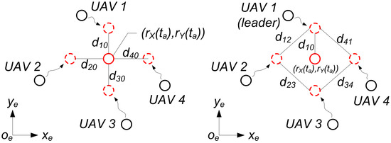
Figure 1. Left: Intuitive desired motion trajectories for quadrotors. Right: Available desired motion trajectories using neighbor-based states.

However, in decentralized formation control, the RFT $r(t)$ is not available for the followers, therefore, it is not possible to design the formation tracking controller using the errors ${\overline{X}}_i^d-X_i$ and ${\overline{Y}}_i^d-Y_i$ for quadrotor i. For the followers, only the neighbors states are available for the formation controller design, as shown in Figure 1 (right). Now, the formation problem becomes: how to find the available guidance vector for quadrotors $i\in \mathcal{V}$ in order to attain the formation task.

Let us make a sum of the relative position state vectors. Note that we drop the explicit expression of time in the expressions for the sake of simplicity. Similar to the foregoing analysis, we still take X for example.

$$\begin{array}{cc}{\displaystyle \sum _{j\in {\mathcal{N}}_i}}(X_i-X_j-d_{ij}^X)& \mathrm{if}i\in \mathcal{V}-{\mathcal{V}}_L\\ {\displaystyle \sum _{j\in {\mathcal{N}}_i}}(X_i-X_j-d_{ij}^X)+X_i-r_X-d_{i0}^X& \mathrm{if}i\in {\mathcal{V}}_L\end{array}$$

(29)

The inter-distance satisfies $d_{ij}^X=d_{i0}^X-d_{j0}^X$. Then, Equation (29) can be rewritten as follows

$$\begin{array}{c}{\displaystyle \sum _{j\in {\mathcal{N}}_i}}(X_i-r_X-d_{i0}^X-(X_j-r_X-d_{j0}^X)),\mathrm{if}i\in \mathcal{V}-{\mathcal{V}}_L\\ {\displaystyle \sum _{j\in {\mathcal{N}}_i}}(X_i-r_X-d_{i0}^X-(X_j-r_X-d_{j0}^X))+X_i-r_X-d_{i0}^X,\mathrm{if}i\in {\mathcal{V}}_L\end{array}$$

Then, the guidance vector for each quadrotor is given as follows

$$X_i^d=\left\{\begin{array}{c}\frac{1}{|{\mathcal{N}}_i|}{\displaystyle \sum _{j\in {\mathcal{N}}_i}}(X_j+d_{ij}^X),\mathrm{if}i\in \mathcal{V}-{\mathcal{V}}_L\\ \frac{1}{|{\mathcal{N}}_i|+1}\left({\displaystyle \sum _{j\in {\mathcal{N}}_i}}(X_j+d_{ij}^X)+r_X+d_{i0}^X\right),\mathrm{if}i\in {\mathcal{V}}_L\end{array}\right.$$

(30)

We then observe that $X_i^d$ is available for quadrotor i, since $X_i^d$ is composed only by neighbors states.

$$\begin{array}{c}\hfill X_i-X_i^d=\left\{\begin{array}{c}\frac{1}{|{\mathcal{N}}_i|}{\displaystyle \sum _{j\in {\mathcal{N}}_i}}\left((X_i-{\overline{X}}_i^d)-(X_j-{\overline{X}}_i^d)\right),\mathrm{if}i\in \mathcal{V}-{\mathcal{V}}_L\\ \frac{1}{|{\mathcal{N}}_i|+1}\left({\displaystyle \sum _{j\in {\mathcal{N}}_i}}\left((X_i-{\overline{X}}_i^d)-(X_j-{\overline{X}}_i^d)\right)+X_i-{\overline{X}}_i^d\right),\mathrm{if}i\in {\mathcal{V}}_L\end{array}\right.\end{array}$$

(31)

Then, according to definition of normalized interaction matrix in (2), we can rewrite Equation (31) in matrix form for all the quadrotors as follows

$$\left[\begin{array}{c}{X}_1-X_1^d\\ ⋮\\ X_n-X_n^d\end{array}\right]=\overline{G}\left[\begin{array}{c}{X}_1-{\overline{X}}_1^d\\ ⋮\\ X_n-{\overline{X}}_n^d\end{array}\right]$$

(32)

where $\overline{G}$ represents the normalized interaction matrix.

According to Corollary 2 and the definition in Equation (2), we know that $\overline{G}$ is invertible if each connected sub-graph of the multi-quadrotor system has at least one leader. Therefore, the formation task is achieved, i.e., ${\left[X_1-{\overline{X}}_1^d,\cdots ,X_n-{\overline{X}}_n^d\right]}^T\to \mathbf{0}$, as long as each quadrotor can precisely track the guidance vector $X_i^d(t)$ and $Y_i^d(t)$, i.e., vector $\left[X_1-X_1^d,\cdots ,X_n-X_n^d\right]\to \mathbf{0}$, and $\left[Y_1-Y_1^d,\cdots ,Y_n-Y_n^d\right]\to \mathbf{0}$.

4.2. Convergence Analysis

Now, the guidance vector ${[X_i^d,Y_i^d,Z_i^d,{\psi }_i^d]}^T$ for each quadrotor is obtained (we note that $Z_i^d$ and ${\psi }_i^d$ are set constant, so omitted here). Their higher-order derivatives are estimated by using finite-time observer (20) in an aggressive formation. Then, these estimated derivatives are used as feedforwards in Equation (17), composing controller (12).

In practice, the estimation errors are usually high at $t=0$ s, when the initial states of the observer may greatly deviate from the real values. In order to avoid the instability caused by the big initial deviation of the observer, we implement saturation functions to the estimated high-order derivatives to prevent great observation errors at the beginning.

To avoid the instability of quadrotors caused by the great initial observation error, we propose a modified controller in Equation (33) using the saturation function as follows

$$\begin{array}{cc}\hfill v_{i1}={\sigma }_{b4}({\widehat{\stackrel{⃜}{X}}}_i^d)-k_{4X}(\dot{{\theta }_i}g-{\sigma }_{b3}(({\widehat{\stackrel{⃛}{X}}}_i^d)))& -k_{3X}({\theta }_{i}g-{\sigma }_{b2}({\hat{\ddot{X}}}_i^d))\hfill \\ \hfill & -k_{2X}({\dot{X}}_i-{\sigma }_{b1}({\hat{\dot{X}}}_i^d))-k_{1X}(X_i-X_i^d)\hfill \\ \hfill v_{i2}={\sigma }_{b4}({\widehat{\stackrel{⃜}{Y}}}_i^d)-k_{4Y}(-{\dot{\varphi }}_{i}g-{\sigma }_{b3}({\widehat{\stackrel{⃛}{Y}}}_i^d))& -k_{3Y}(-{\varphi }_{i}g-{\sigma }_{b2}({\widehat{\ddot{Y}}}_i^d))\hfill \\ \hfill & -k_{2Y}({\dot{Y}}_i-{\sigma }_{b1}({\widehat{\dot{Y}}}_i^d))-k_{1Y}(Y_i-Y_i^d)\hfill \end{array}$$

(33)

The analysis of the convergence is given by the following theorem.

Theorem 2.

Consider the quadrotors with dynamics (8) are controlled by the formation controller (12) composed by (33). The bounds are chosen as follows,

$$b_j=\left\{\begin{array}{ccc}{\hslash }_j,& \mathit{when}& t\le T_{convergence}\\ \infty & \mathit{when}& t>T_{convergence}\end{array}\right.$$

(34)

where $j=\{1,2,3,4\}$ and ${\hslash }_j\in {\mathbb{R}}^{+}$. Then, the formation error for each quadrotor is ultimately bounded and converge to the invariant set as follows.

$$S_b=\{e_{X_i}|\parallel e_{X_i}\parallel \le \frac{2\overline{\kappa }\beta {\lambda }_{max}(P)}{{\lambda }_{min}(Q)}\}$$

(35)

where $\overline{\kappa }>0$. Notations P and Q represent some positive-definite matrices.

Proof. 

Using (13), (16), (18) and (33), the closed-loop planar dynamics of a quadrotor yields the following decoupled form.

$$\begin{array}{c}\hfill {\stackrel{⃜}{X}}_i={\sigma }_{b4}({\widehat{\stackrel{⃜}{X}}}_i^d)-k_{4X}({\stackrel{⃛}{X}}_i-{\sigma }_{b3}({\widehat{\stackrel{⃛}{X}}}_i^d))-k_{3X}({\ddot{X}}_i-{\sigma }_{b2}({\widehat{\ddot{X}}}_i^d))-k_{2X}({\dot{X}}_i-{\sigma }_{b1}({\widehat{\dot{X}}}_i^d))-k_{1X}(X_i-X_i^d)\\ \hfill {\stackrel{⃜}{Y}}_i={\sigma }_{b4}({\widehat{\stackrel{⃜}{Y}}}_i^d)-k_{4Y}({\stackrel{⃛}{Y}}_i-{\sigma }_{b3}({\widehat{\stackrel{⃛}{Y}}}_i^d))-k_{3Y}({\ddot{Y}}_i-{\sigma }_{b2}({\ddot{\overline{Y}}}_i^d))-k_{2Y}({\dot{Y}}_i-{\sigma }_{b1}({\widehat{\dot{Y}}}_i^d))-k_{1Y}(Y_i-{\overline{Y}}_i^d)\end{array}$$

Take $X_i$ for example and denote by $e_{X_i}={[X_i-X_i^d,{\dot{X}}_i-{\dot{X}}_i^d,{\ddot{X}}_i-{\ddot{X}}_i^d,{\stackrel{⃛}{X}}_i-{\stackrel{⃛}{X}}_i^d]}^T$. Then, we can write the dynamics of $e_{X_i}$ in state-space form as follows

$${\dot{e}}_{X_i}=A_c{e}_{X_i}+{\delta }_i$$

(36)

where

$$A_c=\left(\begin{array}{cccc}0& 1& 0& 0\\ 0& 0& 1& 0\\ 0& 0& 0& 1& \\ -k_{1X}& -k_{2X}& -k_{3X}& -k_{4X}\end{array}\right)$$

and $\delta ={[0,0,0,{\Delta }_i]}^T$.

$$\begin{array}{c}\hfill {\Delta }_i={\sigma }_{b4}({\widehat{\stackrel{⃜}{X}}}_i^d)-{\stackrel{⃜}{X}}_i^d+k_{4X}({\sigma }_{b3}({\widehat{\stackrel{⃛}{X}}}_i^d)-{\stackrel{⃛}{X}}_i^d)+k_{3X}({\sigma }_{b2}({\widehat{\ddot{X}}}_i^d)-{\ddot{X}}_i)+k_{2X}({\sigma }_{b1}({\widehat{\dot{X}}}_i^d)-{\dot{X}}_i)\end{array}$$

(37)

• When $t\le T_{convergence}$, it is trivial to prove that $\parallel {\delta }_i\parallel =|\Delta |\le {\hslash }_4+|{\stackrel{⃜}{X}}_i^d|+k_{4X}({\hslash }_3+|{\stackrel{⃛}{X}}_i^d|)+k_{3X}({\hslash }_2+|{\ddot{X}}_i|)+k_{2X}({\hslash }_1+|{\dot{X}}_i|)\le \mathbf{d}<\infty$ is bounded, since $r(t)\in C^5({\mathbb{R}}^{+},{\mathbb{R}}^2)$.
• When $t>T_{convergence}$, $b_j=\infty$, the saturations are removed, such that $\Delta ={\widehat{\stackrel{⃜}{X}}}_i^d-{\stackrel{⃜}{X}}_i^d+k_{4X}({\widehat{\stackrel{⃛}{X}}}_i^d-{\stackrel{⃛}{X}}_i^d)+k_{3X}({\widehat{\ddot{X}}}_i^d-{\ddot{X}}_i)+k_{2X}({\widehat{\dot{X}}}_i^d-{\dot{X}}_i)={\kappa }^T{\tilde{x}}_i^d$, where $\kappa ={[0,k_{2X},k_{3X},k_{4X},1]}^T$, its norm is $\parallel \kappa \parallel =\overline{\kappa }$. According to theorem 1, $\parallel {\tilde{x}}_i^d\parallel \le \beta$ when $t>T_{convergence}$. Then, we conclude that $\parallel {\delta }_i\parallel =|{\Delta }_i|=\overline{\kappa }\parallel {\tilde{x}}_i^d\parallel \le \overline{\kappa }\beta <\infty$.

Therefore, the perturbed term $\delta$ in (36) is bounded and satisfying $\parallel {\delta }_i\parallel \le {\delta }_{max}=max\{\mathbf{d},\overline{\kappa }\beta \}$, for all $t\ge t_0$.

The control gains are selected such that $A_c$ is Hurwitz. Since $A_c$ is Hurwitz, there exists a positive-definite matrix P, which solves the Lyapunov equation $A_c^{T}P+P{A}_c=-Q$, for a positive-definite matrix Q. A Lyapunov function is selected as $V=e_{X_i}^{T}P{e}_{X_i}$. Then, its time derivative yields

$$\begin{array}{cc}\hfill \dot{V}=& e_{X_i}^T(A_c^{T}P+P{A}_c)e_{X_i}+2e_{X_i}^{T}P{\delta }_i\le -e_{X_i}^{T}Q{e}_{X_i}+2{\lambda }_{max}(P)\parallel e_{X_i}\parallel \parallel {\delta }_i\parallel \hfill \\ \hfill \le & -{\lambda }_{min}(Q)\parallel e_{X_i}{\parallel }^2+2{\lambda }_{max}(P)\parallel e_{X_i}\parallel \parallel {\delta }_i\parallel =\parallel e_{X_i}\parallel (2{\delta }_{max}{\lambda }_{max}(P)-{\lambda }_{min}(Q)\parallel e_{X_i}\parallel )\hfill \end{array}$$

Then, $\dot{V}<0$, if $\parallel e_{X_i}\parallel >\frac{2{\delta }_{max}{\lambda }_{max}(P)}{{\lambda }_{min}(Q)}$. When $t>T_{convergence}$, according to LaSalle’s invariance principle, for any initial condition $x(t_0)$, the state x will finally stay in the set $S_b=\{e_{X_i}|\parallel e_{X_i}\parallel \le \frac{2\overline{\kappa }\beta {\lambda }_{max}(P)}{{\lambda }_{min}(Q)}\}$. The error $e_{X_i}$ in (36) is ultimately bounded. The same result on Y can be obtained similarly. □

Remark 4.

According to Theorem 2, the tracking error of quadrotor is proportional to the bound β of the observer error after finite time $T_{convergence}$. If the observer error asymptotically converges to zero, then the formation tracking error will also converge to zero asymptotically.

Remark 5.

In practice, before the time instant $T_{convergence}$, the bounds $b_j$ are chosen small enough in order to prevent the unstable dynamics, since the observer error probably enormous, which is generated by great initial deviation.

5. Simulation and Experimental Results

In this subsection, we first use numerical simulation by means of MATLAB to qualitatively illustrate that the formation controller with estimated feedforwards has better performance than that without them. By doing this, we are able to show that our proposed formation controller makes the multi-quadrotor system performing a high bandwidth, such that the aggressive formation is achieved.

Then in the second subsection, the proposed control laws are implemented on the simulator-experiment platform comparing with that using the formation controller without high-order feedforwards.

5.1. Simulation Results

We reconsider the formation of four quadrotors in Figure 1 (left). The reference formation trajectory RFT is given by $r(t)={[3sin(0.1t),3cos(0.1t),1,0]}^T$. The four quadrotors should keep a desired biases w.r.t. RFT defined by $d_{i0}$, $i\in \{1,2,3,4\}$. As shown in Figure 1 (right), quadrotor 3 has two neighbors, i.e., 2 and 4. The quadrotor 3 is expected to keep inter-distances $d_{32}={[\sqrt{2},-\sqrt{2}]}^T$ and $d_{34}={[-\sqrt{2},-\sqrt{2}]}^T$ with respect to 2 and 4. It is easy to verify that $d_{32}=d_{30}-d_{20}$ and $d_{34}=d_{30}-d_{40}$.

The tuning process of the controller gains in Table 2 is given as follows.

Table 2. The controllers parameters.

${\mathit{k}}_{4\mathit{X}}$	${\mathit{k}}_{3\mathit{X}}$	${\mathit{k}}_{2\mathit{X}}$	${\mathit{k}}_{1\mathit{X}}$	${\mathit{k}}_{4\mathit{Y}}$	${\mathit{k}}_{3\mathit{Y}}$	${\mathit{k}}_{2\mathit{Y}}$	${\mathit{k}}_{1\mathit{Y}}$	${\mathit{k}}_{2\mathit{\psi }}$	${\mathit{k}}_{1\mathit{\psi }}$	${\mathit{k}}_{2\mathit{Z}}$	${\mathit{k}}_{1\mathit{Z}}$
1.0	2.5	1.8	1.3	1.0	2.5	1.8	1.3	17.3	10.2	3.1	2.2

• Controller gains tuning on simulator: Let ${\dot{X}}_i^d$, ${\ddot{X}}_i^d$, ${\stackrel{⃛}{X}}_i^d$, ${\stackrel{⃜}{X}}_i^d$, and ${\dot{Y}}_i^d$, ${\ddot{Y}}_i^d$, ${\stackrel{⃛}{Y}}_i^d$, ${\stackrel{⃜}{Y}}_i^d$ be null. Give some small $X_i^d$ and $Y_i^d$, for example a small step signal, then, tune the gains $k_{jX}$ and $k_{jY}$, $j=\{1,2,3,4\}$. Observe the oscillation of the rotation angles during translational motion, adjust the gains $k_{3X}$, $k_{4X}$ and $k_{3Y}$, $k_{4Y}$ to reduce the oscillation.
• Implement the controller gains on real quadrotor: Test on single quadrotor, slightly tune the parameters $k_{1X}$, $k_{2X}$ if necessary. Then, if the performance is satisfied, implement them on the formation tracking control.

The observer gain matrix is selected according to the pole assignment as follows

• Pole assignment: The gains of the observer are dominated by the finite time $T_{converge}$ that we want to have. Once it is fixed, the gains of the observer can be calculated by the technique of pole assignment, such that the nearest pole of $A_o$ to imaginary axis is placed to $-\gamma$.

In the following simulation and experiments, we assume that the position and velocity in the guidance vector are measurable, i.e.,

$$C_t=\left[\begin{array}{cccc}1& 0& 0& 0\\ 0& 1& 0& 0\end{array}\right]$$

the observe gains are selected as follows,

$$L_t={\left[\begin{array}{ccccc}6& 1& 1& 1.02& 0.198\\ 1.804& 9.02& 14.432& 6.675& 0.934\end{array}\right]}^T$$

(38)

Some constant bounds of the saturation functions are selected as $b_4=0.000035$, $b_3=0.00035$, $b_2=0.0035$, and $b_1=\infty$. The saturation functions are introduced to regulate the large initial deviation of the observer. There bounds are tuned progressively until a satisfactory performance is achieved.

We respectively show in Figure 2 and Figure 3 the simulation results (i) without estimation of high-order derivatives and (ii) with estimation of high-order derivatives. We observe from Figure 2 that the quadrotors track the RFT with delays and the inter-distances are not well maintained. On the contrary, in Figure 3, the delays are small and the quadrotors keep around the desired inter-distances.

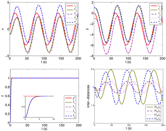
Figure 2. Rigid formation of 4 quadrotors without high-order derivatives estimation, the objective is to track the RFT $r(t)$ and meanwhile keep inter-distance between quadrotors.

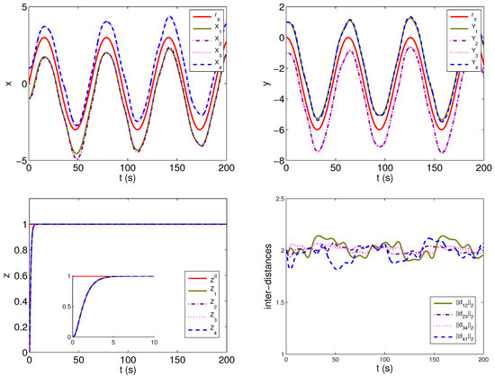
Figure 3. Rigid formation of 4 quadrotors with high-order derivatives estimation, the objective is to track the RFT $r(t)$ and meanwhile keep inter-distance between quadrotors.

In the following subsection, we will implement the formation control protocol on the real-time simulator-experiment platform.

5.2. Experimental Setup

Heudiasyc laboratory (In the Université de Technologie de Compiègne) has developed a PC-based simulator-experiment framework (This framework is primarily designed and developed by engineer Guillaume Sanahuja under the help of other colleagues and PhD students in Heudiasyc laboratory) for controlling quadrotors in real-time. The programs (written in C++) running in the quadrotors are the same, both in the simulator and in the embedded processors of real quadrotors. The goal of the framework is to firstly validate a program on the simulator before implementing on real quadrotors, in order to avoid destroying the real drones. It is important to note that within this framework, the control algorithms are implemented on the quadrotors rather than on a PC. There does not exist a central controller that sends control signals to the quadrotors.

In the simulator, the complete quadrotor dynamics are used. The flight of the quadrotors are animated in a virtual 3D environment, which permits us to observe the behavior of the quadrotors under some formation control laws. This framework permits the simulation to reflect better the real-time experiment. Both the simulator and the real-time experiment share the ground station interface on the PC, which is responsible for displaying and sending instructions such as taking off and landing.

The experimental setup is shown in Figure 4. In the experiments, the motion capture system Optitrack is used to localize the quadrotors in the formation. The ArDrone2 quadrotors manufactured by Parrot are used for real-time experiments.

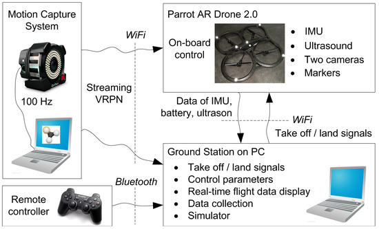
Figure 4. The experimental setup of the real-time experiments.

The procedure of using the simulator-experiment framework is stated as follows:

• Program the algorithms by using C++.
• Compile the program into executable files for the quadrotors in the simulator and for the real quadrotors.
• Test the algorithm in the simulator, adjust the parameters of the controller.
• Send the executable file to each quadrotor.
• Carry out the real-time experiment.

Remark 6.

Although the system Optitrack is a global localization system, we just use it to obtain the coordinates or inter-distances of the quadrotors. For instance, a quadrotor can use its on-board cameras to detect other quadrotors and calculate their inter-distances. Additionally, the self-localization can be realized by using GPS or other sensors (laser, etc.). The system Optitrack is used here to simplify the study.

5.3. Real-Time Experiments on Simulator-Experiment Platform

In these experiments are the formation task of four quadrotors, where quadrotor 1 is a leader. The objective is to track the trajectory $r(t)$ with constant biases $d_{10}={[0,\sqrt{2}]}^T$, $d_{20}={[-\sqrt{2},0]}^T$, $d_{30}={[0,-\sqrt{2}]}^T$ and $d_{40}={[\sqrt{2},0]}^T$.

Two tests are carried out on the simulator for the sake of comparison. In both tests, the objective is to track a circular trajectory (radius: 2 m; maximum linear velocity: $1.3$ m/s; linear acceleration $0.1$ m/s${}^2$).

In the formation control without high-order feedforwards, the gains are chosen by $k_p=1.5$ and $k_d=0.1$. We note that these gains are not arbitrarily chosen. For the fairness of comparison, we tune the parameters on the simulator to obtain the gains with best performance.

We proposed a nonlinear-flatness-based formation controller in (12), where the high-order derivatives are estimated by using (20). In the simulator and the experiment, the control frequency is 50 Hz. Then, the states of the observer (20) are updated as follows

$${\widehat{X}}_i^d(k+1)=(I_5+T·A_t){\widehat{X}}_i^d(k)-T·L_t·C_t({\widehat{X}}_i^d(k)-X_i^d(k))$$

where $T=\frac{1}{50}=0.02$ s. The observer gains are given by (38).

In Figure 5, we observe from Figure 5 that even at the beginning (when $t<20$ s), the quadrotors are able to follow the given trajectory, after 20 s, the performance becomes not satisfactory, although the formation errors keep stable.

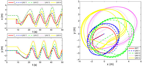
Figure 5. Formation control without high-order feedforwards.

On the contrary, by using the proposed formation control with the same controller gains, the performance is greatly improved and the quadrotors can always follow the given trajectory (see Figure 6).

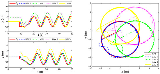
Figure 6. Our proposed formation control.

The desired altitude is 1 m for all the quadrotors. The curves of the altitudes of the quadrotors are given in Figure 7. We can observe from Figure 7 (left) that the altitude of the quadrotor 2 oscillates after $t=25$ s. It is important to note that this phenomena is caused by the actuator saturation of the quadrotors. Considering this problem, we have proposed several bounded formation controllers such as in [13], which will not be detailed in the current paper.

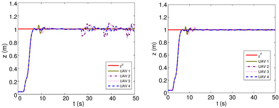
Figure 7. Altitudes of the quadrotors. Left: Formation control without high-order feedforwards. Right: Our proposed formation control.

Figure 8 shows the animation in the simulator. On the left of Figure 8, the formation control without high-order feedforwards is used, where the quadrotors fail to preserve the rectangle formation pattern after several second of flight. On the contrary, the nonlinear-flatness-based formation control can preserve the rectangle formation and track the RFT that is only given to the leader.

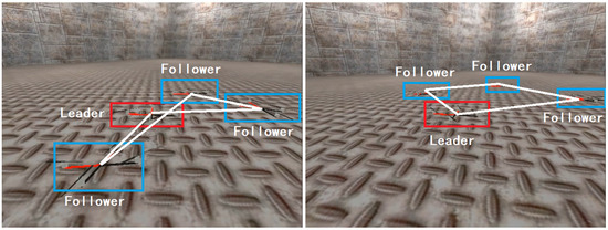
Figure 8. Four quadrotors with rectangle formation pattern, tracking a circular trajectory, using formation control without high-order feedforwards (left), and the proposed formation control (right).

A real-time experiment is also given in Figure 9, where four quadrotors are used in the tests. The reference is a circular trajectory. Two tests are given for comparison. We can observe that by using our proposed controller, the formation trajectory is more precisely followed. Figure 10 shows a photo of flight in a real-time experiment.

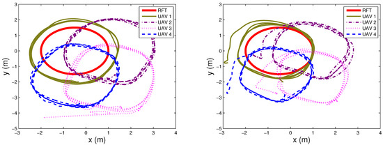
Figure 9. The real-time four quadrotors formation. Left: Formation control without high-order feedforwards; Right: our proposed method.

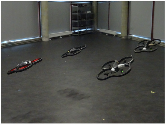
Figure 10. A snap of the real flight of four quadrotors’ formation, tracking a circular trajectory while maintaining a rectangle pattern.

6. Conclusions

In this paper, a nonlinear-flatness-based formation control with feedforwards of estimated high-order guidance vector (neighbors’ states, and RFT, if the quadrotor is a leader) derivatives is developed. The formation controller is decentralized, which is designed based on neighbors’ states. In order to attain an aggressive formation, an extended finite-time observer of the guidance vector is investigated. In order to deal with the great initial deviation of the estimated states, the saturated feedforwards are developed. Then, the convergence of the formation tracking error is analyzed. Furthermore, the proposed formation control is illustrated by simulation and real-time experiment by means of MATLAB and the simulator-experiment platform, comparing with the formation control without high-order feedforwards. Both simulation and real-time experimental results show that the aggressive formation performance is improved by using our proposed formation controller.

One of the directions of the future work is to implement the proposed control with advanced nonlinear control methods, in order to deal with the effects of nonlinearities (uncertainties), to achieve asymptotic finite-time convergence, to control explicitly the formation tracking speed, etc.

Appendix A.1. Proof of Proposition 3

Proof of Proposition 3. 

According to (5), we obtain that

$$F_{T_i}=\frac{({\ddot{Z}}_i+g)m}{cos{\theta }_{i}cos{\varphi }_i}$$

(A1)

Replacing $F_{T_i}$ by (A1) in the first two equations in (5), we obtain

$$\begin{array}{c}{\ddot{X}}_i=\left(sin{\psi }_i\frac{tan{\varphi }_i}{cos{\theta }_i}+cos{\psi }_{i}tan{\theta }_i\right)({\ddot{Z}}_i+g)\hfill \\ {\ddot{Y}}_i=\left(sin{\psi }_{i}tan{\theta }_i-cos{\psi }_i\frac{tan{\varphi }_i}{cos{\theta }_i}\right)({\ddot{Z}}_i+g)\hfill \end{array}$$

(A2)

We assume that ${\ddot{Z}}_i\ne -g$. Then, according to Equation (A2), we obtain that

$$\begin{array}{c}\hfill \frac{tan{\varphi }_i}{cos{\theta }_i}=\frac{{\ddot{X}}_{i}sin{\psi }_i-{\ddot{Y}}_{i}cos{\psi }_i}{{\ddot{Z}}_i+g}\\ \hfill tan{\theta }_i=\frac{{\ddot{X}}_{i}cos{\psi }_i+{\ddot{Y}}_{i}sin{\psi }_i}{{\ddot{Z}}_i+g}\end{array}$$

Then, we have

$$\begin{array}{cc}\hfill {\theta }_i=arctan& \left(\frac{{\ddot{X}}_{i}cos{\psi }_i+{\ddot{Y}}_{i}sin{\psi }_i}{{\ddot{Z}}_i+g}\right)\hfill \\ \hfill {\varphi }_i=arctan& \left(\frac{{\ddot{X}}_{i}sin{\psi }_i-{\ddot{Y}}_{i}cos{\psi }_i}{{\ddot{Z}}_i+g}cos\left(arctan\left(\frac{{\ddot{X}}_{i}cos{\psi }_i+{\ddot{Y}}_{i}sin{\psi }_i}{{\ddot{Z}}_i+g}\right)\right)\right)\hfill \end{array}$$

(A3)

Since ${ϝ}_i={[{\mathcal{X}}_i^T,{\psi }_i]}^T$, we denote ${ϝ}_{i1}=X_i$, ${ϝ}_{i2}=Y_i$, ${ϝ}_{i3}=Z_i$ and ${ϝ}_{i4}={\psi }_i$. Then, the state of the quadrotor ${\varkappa }_i$ yields

$$\begin{array}{cc}\hfill X_i=& {ϝ}_{i1},Y_i={ϝ}_{i2},Z_i={ϝ}_{i3},\hfill \\ \hfill {\dot{X}}_i=& {\dot{ϝ}}_{i1},{\dot{Y}}_i={\dot{ϝ}}_{i2},{\dot{Z}}_i={\dot{ϝ}}_{i3},\hfill \\ \hfill {\theta }_i=& arctan\left(\frac{{\ddot{ϝ}}_{i1}cos{ϝ}_{i4}+{\ddot{ϝ}}_{i2}sin{ϝ}_{i4}}{{\ddot{ϝ}}_{i3}+g}\right)\hfill \\ \hfill {\varphi }_i=& arctan\left(\frac{{\ddot{ϝ}}_{i1}sin{ϝ}_{i4}-{\ddot{ϝ}}_{i2}cos{ϝ}_{i4}}{{\ddot{ϝ}}_{i3}+g}cos\left(arctan\left(\frac{{\ddot{ϝ}}_{i1}cos{ϝ}_{i4}+{\ddot{ϝ}}_{i2}sin{ϝ}_{i4}}{{\ddot{ϝ}}_{i3}+g}\right)\right)\right)\hfill \\ \hfill {\psi }_i=& {ϝ}_{i4}\hfill \\ \hfill {\dot{\theta }}_i=& {\left(arctan\left(\frac{{\ddot{ϝ}}_{i1}cos{ϝ}_{i4}+{\ddot{ϝ}}_{i2}sin{ϝ}_{i4}}{{\ddot{ϝ}}_{i3}+g}\right)\right)}^{(1)}\hfill \\ \hfill {\dot{\varphi }}_i=& {\left(arctan\left(\frac{{\ddot{ϝ}}_{i1}sin{ϝ}_{i4}-{\ddot{ϝ}}_{i2}cos{ϝ}_{i4}}{{\ddot{ϝ}}_{i3}+g}cos\left(arctan\left(\frac{{\ddot{ϝ}}_{i1}cos{ϝ}_{i4}+{\ddot{ϝ}}_{i2}sin{ϝ}_{i4}}{{\ddot{ϝ}}_{i3}+g}\right)\right)\right)\right)}^{(1)}\hfill \\ \hfill {\dot{\psi }}_i=& {\dot{ϝ}}_{i4}\hfill \end{array}$$

(A4)

Equation (A4) imply that the state ${\varkappa }_i$ can be parameterized by variable ${ϝ}_i$ and its derivatives. According to (9), the output $y_i$ is in terms of ${\mathcal{X}}_i$, ${\dot{\mathcal{X}}}_i$, ${\mathrm{\Theta }}_i$ and ${\dot{\mathrm{\Theta }}}_i$, therefore $y_i$ can also be parameterized by ${ϝ}_i$. Additionally, according to (8), the control input $u_i$ is in terms of $Z_i$, ${\dot{Z}}_i$, ${\mathrm{\Theta }}_i$, ${\dot{\mathrm{\Theta }}}_i$ and ${\ddot{\mathrm{\Theta }}}_i$. Therefore, the variable ${ϝ}_i$ is the flat output of system (8). □

Appendix A.2. Model Simplification

According to Equation (A2), we can obtain the following equations

$$\begin{array}{cc}\hfill {\theta }_i=arctan& \left(\frac{{\ddot{X}}_{i}cos{\psi }_i+{\ddot{Y}}_{i}sin{\psi }_i}{{\ddot{Z}}_i+g}\right)\hfill \\ \hfill {\varphi }_i=arctan& \left(\frac{{\ddot{X}}_{i}sin{\psi }_i-{\ddot{Y}}_{i}cos{\psi }_i}{{\ddot{Z}}_i+g}cos\left(arctan\left(\frac{{\ddot{X}}_{i}cos{\psi }_i+{\ddot{Y}}_{i}sin{\psi }_i}{{\ddot{Z}}_i+g}\right)\right)\right)\hfill \end{array}$$

(A5)

Without loss of generality, we assume that the yaw angle is controlled at origin, and the altitude is stabilized at some constant value, then,

$$\begin{array}{ccc}{\theta }_i=arctan\left({\ddot{X}}_i/g\right)& \mathrm{and}& {\varphi }_i=arctan\left(-({\ddot{Y}}_i/g)cos{\theta }_i\right)\end{array}$$

(A6)

Furthermore, considering Assumption 1, we obtain that

$$\begin{array}{c}{\ddot{X}}_i={\theta }_{i}g+{\Delta }_{X_i}\hfill \\ {\ddot{Y}}_i=-{\varphi }_{i}g+{\Delta }_{Y_i}\hfill \end{array}$$

(A7)

where the nonlinearities ${\Delta }_{X_i}$ and ${\Delta }_{Y_i}$ are bounded since the absolute values of ${\theta }_i$ and ${\varphi }_i$ are bounded within ${30}^{\circ }$ by assumption 1. Then, we know that (A7) is Lyapunov stable, if the simplified system (16) is asymptotically stable.

References

- Liu, H.; Ma, T.; Lewis, F.L.; Wan, Y. Robust Formation Control for Multiple Quadrotors with Nonlinearities and Disturbances. IEEE Trans. Cybern. 2020, 50, 1362–1371. [Google Scholar] [CrossRef] [PubMed]
- Villa, D.K.D.; Brandão, A.S.; Sarcinelli-Filho, M. Path-Following and Attitude Control of a Payload Using Multiple Quadrotors. In Proceedings of the 2019 19th International Conference on Advanced Robotics (ICAR), Belo Horizonte, Brazil, 2–6 December 2019; pp. 535–540. [Google Scholar] [CrossRef]
- Wang, Z.; Singh, S.; Pavone, M.; Schwager, M. Cooperative Object Transport in 3D with Multiple Quadrotors Using No Peer Communication. In Proceedings of the 2018 IEEE International Conference on Robotics and Automation (ICRA), Brisbane, Australia, 21–25 May 2018; pp. 1064–1071. [Google Scholar] [CrossRef]
- Villa, D.K.D.; Brandão, A.S.; Sarcinelli-Filho, M. Rod-shaped payload transportation using multiple quadrotors. In Proceedings of the 2019 International Conference on Unmanned Aircraft Systems (ICUAS), Atlanta, GA, USA, 11–14 June 2019; pp. 1036–1040. [Google Scholar] [CrossRef]
- Kushleyev, A.; Kumar, V.; Mellinger, D. Towards a Swarm of Agile Micro Quadrotors. In Proceedings of the Robotics: Science and Systems, Vilamoura, Portugal, 7–12 October 2012. [Google Scholar]
- Sreenath, K.; Kumar, V. Dynamics, Control and Planning for Cooperative Manipulation of Payloads Suspended by Cables from Multiple Quadrotor Robots. In Proceedings of the Robotics: Science and Systems, Berlin, Germany, 24–28 June 2013. [Google Scholar]
- Cao, Y.; Yu, W.; Ren, W.; Chen, G. An Overview of Recent Progress in the Study of Distributed Multi-Agent Coordination. IEEE Trans. Ind. Inform. 2013, 9, 427–438. [Google Scholar] [CrossRef]
- Shao, X.; Tian, B.; Li, D. Neural Dynamic Surface Containment Control for Multiple Quadrotors. In Proceedings of the 2019 IEEE International Conference on Unmanned Systems (ICUS), Beijing, China, 17–19 October 2019; pp. 373–378. [Google Scholar] [CrossRef]
- Katt, C.; Castaneda, H. Containment Control Based on Adaptive Sliding Mode for a MAV Swarm System under perturbation. In Proceedings of the 2019 International Conference on Unmanned Aircraft Systems (ICUAS), Atlanta, GA, USA, 11–14 June 2019; pp. 270–275. [Google Scholar] [CrossRef]
- Meng, Z.; Ren, W.; You, Z. Distributed finite-time attitude containment control for multiple rigid bodies. Automatica 2010, 46, 2092–2099. [Google Scholar] [CrossRef]
- Roldao, V.; Cunha, R.; Cabecinhas, D.; Silvestre, C.; Oliveira, P. A leader-following trajectory generator with application to quadrotor formation flight. Robot. Auton. Syst. 2014, 62, 1597–1609. [Google Scholar] [CrossRef]
- Mercado, D.A.; Castro, R.; Lozano, R. Quadrotors flight formation control using a leader-follower approach. In Proceedings of the 2013 European Control Conference (ECC), Zurich, Switzerland, 17–19 July 2013; pp. 3858–3863. [Google Scholar] [CrossRef]
- Hou, Z.; Fantoni, I. Interactive Leader Follower Consensus of Multiple Quadrotors Based on Composite Nonlinear Feedback Control. IEEE Trans. Control Syst. Technol. 2018, 26, 1732–1743. [Google Scholar] [CrossRef]
- Saber, R.; Murray, R. Flocking with obstacle avoidance: Cooperation with limited communication in mobile networks. In Proceedings of the 42nd IEEE Conference on Decision and Control, Maui, HI, USA, 9–12 December 2003; Volume 2, pp. 2022–2028. [Google Scholar] [CrossRef]
- Olfati-Saber, R.; Fax, J.; Murray, R. Consensus and Cooperation in Networked Multi-Agent Systems. Proc. IEEE 2007, 95, 215–233. [Google Scholar] [CrossRef]
- Turpin, M.; Michael, N.; Kumar, V. Trajectory design and control for aggressive formation flight with quadrotors. Auton. Robots 2012, 33, 143–156. [Google Scholar] [CrossRef]
- Zhao, D.; Krishnamurthi, J.; Gandhi, F.; Mishra, S. Differential flatness based trajectory generation for time-optimal helicopter shipboard landing. In Proceedings of the 2018 Annual American Control Conference (ACC), Milwaukee, WI, USA, 27–29 June 2018; pp. 2243–2250. [Google Scholar] [CrossRef]
- Son, C.Y.; Jang, D.; Seo, H.; Kim, T.; Lee, H.; Kim, H.J. Real-time Optimal Planning and Model Predictive Control of a Multi-rotor with a Suspended Load. In Proceedings of the 2019 International Conference on Robotics and Automation (ICRA), Montreal, QC, Canada, 20–24 May 2019; pp. 5665–5671. [Google Scholar] [CrossRef]
- Zeng, J.; Kotaru, P.; Mueller, M.W.; Sreenath, K. Differential Flatness Based Path Planning with Direct Collocation on Hybrid Modes for a Quadrotor With a Cable-Suspended Payload. IEEE Robot. Autom. Lett. 2020, 5, 3074–3081. [Google Scholar] [CrossRef]
- Hou, Z.; Xu, J.; Zhang, G. Interaction Matrix Based Analysis and Asymptotic Cooperative Control of Multi-agent Systems. Int. J. Control Autom. Syst. 2020, 18, 1103–1115. [Google Scholar] [CrossRef]
- Irofti, D. An anticipatory protocol to reach fast consensus in multi-agent systems. Automatica 2020, 113, 108776. [Google Scholar] [CrossRef]
- Liu, H.; Tian, Y.; Lewis, F.L.; Wan, Y.; Valavanis, K.P. Robust formation tracking control for multiple quadrotors under aggressive maneuvers. Automatica 2019, 105, 179–185. [Google Scholar] [CrossRef]
- Zhao, B.; Wang, D.; Shi, G.; Liu, D.; Li, Y. Decentralized Control for Large-Scale Nonlinear Systems with Unknown Mismatched Interconnections via Policy Iteration. IEEE Trans. Syst. Man Cybern. Syst. 2018, 48, 1725–1735. [Google Scholar] [CrossRef]
- Bhat, S.P.; Bernstein, D.S. Finite-Time Stability of Continuous Autonomous Systems. SIAM J. Control Optim. 2000, 38, 751–766. [Google Scholar] [CrossRef]
Publisher’s Note: MDPI stays neutral with regard to jurisdictional claims in published maps and institutional affiliations. |
© 2021 by the authors. Licensee MDPI, Basel, Switzerland. This article is an open access article distributed under the terms and conditions of the Creative Commons Attribution (CC BY) license (http://creativecommons.org/licenses/by/4.0/).