Integrating Dilated Convolution into DenseLSTM for Audio Source Separation

Abstract

Herein, we proposed a multi-scale multi-band dilated time-frequency densely connected convolutional network (DenseNet) with long short-term memory (LSTM) for audio source separation. Because the spectrogram of the acoustic signal can be thought of as images as well as time series data, it is suitable for convolutional recurrent neural network (CRNN) architecture. We improved the audio source separation performance by applying the dilated block with a dilated convolution to CRNN architecture. The dilated block has the role of effectively increasing the receptive field in the spectrogram. In addition, it was designed in consideration of the acoustic characteristics that the frequency axis and the time axis in the spectrogram are changed by independent influences such as speech rate and pitch. In speech enhancement experiments, we estimated the speech signal using various deep learning architectures from a signal in which the music, noise, and speech were mixed. We conducted the subjective evaluation on the estimated speech signal. In addition, speech quality, intelligibility, separation, and speech recognition performance were also measured. In music signal separation, we estimated the music signal using several deep learning architectures from the mixture of the music and speech signal. After that, the separation performance and music identification accuracy were measured using the estimated music signal. Overall, the proposed architecture shows the best performance compared to other deep learning architectures not only in speech experiments but also in music experiments.

1. Introduction

In a real environment, humans hear several mixed signals simultaneously. In these situations, we can selectively attend to a signal we want, effectively segregating a target from the perceived mixture. This is the so-called auditory scene analysis or the cocktail effect problem [1], which is the main topic of this paper. In particular, when signals such as unwanted noise are mixed with the target signal, system performance is degraded, and the necessity of this study is emphasized [2,3]. Audio source separation is used to estimate the target signal, such as speech and music, when the target signal and other signals are mixed. If the target signal to be estimated is speech, it is the speech enhancement task; if the target signal is music, it is the music signal separation task.

In the conventional method of audio source separation with linear characteristics, non-negative matrix factorization (NMF) [4] is used not only for speech enhancement but for music source separation tasks [5,6,7]. NMF is an algorithm that decomposes a signal into two non-negative matrices that are a basis matrix representing independent characteristics and an activation matrix for each characteristic [4]. Each component of the signal can be separated using the basis matrix learned in the training process. Recently, deep learning, which has non-linear characteristics, showed better results than the traditional NMF method in audio source separation [8,9,10,11,12,13,14]. Deep learning has several representative architectures, such as the fully connected neural network (FCNN) [15], convolutional neural network (CNN) [16], and recurrent neural network (RNN) [17]. Often, these architectures are modified or combined to design a new architecture suitable for the task. FCNN architecture, which is the most basic deep learning architecture, is an architecture in which the nodes of each layer are fully connected [15], while the CNN designed for image processing is an architecture that convolves filters as a weight sharing method [16]. In addition, an RNN suitable for processing time series data is characterized by accumulating and using the information of the input data in chronological order within the architecture [17].

Many studies have shown better performance than the FCNN by using bidirectional long short-term memory (BLSTM) and CNN architectures [18,19,20,21,22,23,24,25]. Long short-term memory (LSTM) has a memory cell involved in inputs and outputs to store longer time series information than vanilla RNN [26]. BLSTM architecture determines the output by combining the forward time series information and the backward time series information of the LSTM [27]. The CNN architecture that shares weights can be used to design deeper layers of networks with the same parameters, which means that CNNs can learn more complex patterns of filters than FCNN architecture.

Recently, the convolutional recurrent neural network (CRNN) architecture [28] that uses CNNs suitable for image processing and RNNs suitable for time series data processing in one architecture at the same time shows better performance than other CNN, RNN, and BLSTM architectures [29,30,31]. In the CRNN architecture, LSTM or BLSTM architectures of the RNN series, which has better performance than vanilla RNN, is used. The parameters of the CNN are learned to estimate a filter for the target, and also the parameters of the RNN are learned to store the target information using time series information [28]. In the spectrogram of the acoustic signal, the target pattern shows slightly different characteristics depending on the frequency axis but appears at various locations along the time axis. Therefore, it is suitable for the translation-equivariance characteristics of the CNN architecture. In addition, since the time series data is along the time axis, it is suitable for the RNN architecture [29,30,31]. When the spectrogram is an input, the CRNN architecture first obtains a feature map through the CNN, and then features using time series information can be obtained from the RNN since time series information can still be used along the time axis of the feature map. Therefore, it is ideal to learn various patterns together using a CRNN architecture in an acoustic signal, and it shows good performance [29,30,31].

The CNN-based architectures for music source separation have an encoder-decoder architecture through down-sampling and up-sampling [23,24,25]. This encoder-decoder style architecture is intended to effectively increase the receptive field [32] and utilize the contextual information extracted from a wider time range of input data. In our previous study [33], we created a dilated block that effectively increased the receptive field by using a dilated convolution [34], which is suitable for the acoustic characteristics. The dilated convolution has the advantage of having a larger receptive field with the same number of parameters by adding an empty space between the filter nodes [34]. In order to apply the dilated convolution more appropriately to the spectrogram, the dilated block of the previous study was designed to arrange the dilated convolution of the time axis, the dilated convolution of the frequency axis, and the standard convolution in parallel [33]. The architecture where the dilated block is added in front of the dense block is called a dilated dense block. A dilated time-frequency DenseNet (DilDenseNet), which we designed using a dilated block, confirmed that it improves the performance in a music signal separation task [33].

In this study, we proposed a multi-scale multi-band dilated time-frequency DenseNet with LSTM (MMDilDenseLSTM) architecture for source separation. In addition to the encoder-decoder style, we applied a dilated block to CRNN architecture in order to expand the receptive field more effectively. We experimented with speech enhancement and music signal separation to evaluate the performance of MMDilDenseLSTM in comparison with other deep learning architectures. In the speech enhancement task, we performed subjective evaluation for the enhanced speech signal. In addition, we also measured speech quality, intelligibility, separation performance, and speech recognition accuracy. In the music separation task, separation performance and music identification performance were tested. We found that separation performance did not always correlate with speech recognition performance or music identification performance. To investigate the cause of this uncorrelated relationship, we analyzed the separated signal by plotting an intuitive feature of the music identification system on the spectrogram. In the speech and music experiments, the proposed architecture, which effectively increased the receptive field in CRNN architecture, showed the best performance overall compared to the existing deep learning architectures.

We first introduce related works in Section 2 and then explain the proposed MMDilDenseLSTM in detail in Section 3. In Section 4, we present our experimental results. Finally, we offer conclusions in Section 5.

2. Related Works

Gated residual network (GRN), which is a CNN-based architecture, consists of a frequency-dilated module that extends the receptive field on the frequency axis, a time-dilated module that increases the receptive field on the time axis, and, finally, a prediction module that outputs a mask of the same size as the input [35]. In particular, the GRN architecture is a deeper network that has a wide receptive field along the time axis by arranging several time-dilated modules, and this architecture has shown better performance than vanilla RNN and BLSTM based on a fully connected layer in speech enhancement [35].

Recently, the multi-scale multi-band DenseNet (MMDenseNet) architecture using densely connected convolutional networks (DenseNet) [36] showed good performance in music source separation [25]. In the DenseNet architecture, since the final output feature map includes the input and the output feature map of each layer, it has the advantage that a lot of information is included in the feed-forward process. In addition, there is an advantage that the gradient vanishing problem can be untangled because an error is simultaneously transmitted to each layer without passing through nodes in the error backpropagation process [36]. MMDenseNet has a multi-scale DenseNet (MDenseNet) architecture in parallel for each divided frequency band. The MDenseNet architecture has a process of obtaining low-dimensional features by repeating a dense block of DenseNet and down-sampling, and then restoring the original size by repeating dense block and up-sampling. For simplicity, the process of representing the input data as a low-dimensional feature is called an encoding process, and the process of restoring the low-dimensional feature obtained in the encoding process to its original size is called a decoding process. Recently, the best performance of the music source separation task is MMDenseNet with LSTM (MMDenseLSTM) [31], which combines BLSTM with CNN-based MMDenseNet [25]. MMDenseLSTM is a CRNN architecture in which a BLSTM architecture is added after several dense block of MMDenseNet. Similar to speech enhancement tasks, the CRNN architecture is currently the best performing architecture.

In the time domain, end-to-end methods not relying on spectrogram have been successfully applied to audio source separation [37,38]. There are two drawbacks when the spectrogram is used as input. First, it consumes time to extract the spectrogram and restore it to a signal. Second, the phase information of the mixture used in the restoration process causes distortion. Recently, one of the end-to-end methods, Wave-U-Net, actually did not show good performance in music signal separation [37], whereas the other Conv-TasNet showed very good performance in the speaker separation task [38]. From these previous study results, we took the approach of using spectrogram as and input and will pursue the end-to-end methods in the future research work.

3. Proposed Architecture

The proposed architecture is presented in three steps. First, we introduced a novel dilated dense block that combines the dilated block [33] with the dense block of DenseNet. The dilated dense block was integrated into the multi-scale DenseLSTM (MDenseLSTM) architecture [31] to create a multi-scale dilated time-frequency DenseLSTM (MDilDenseLSTM). Finally, we combined multiple MDilDenseLSTM covering different frequency bands into the proposed architecture, MMDilDenseLSTM.

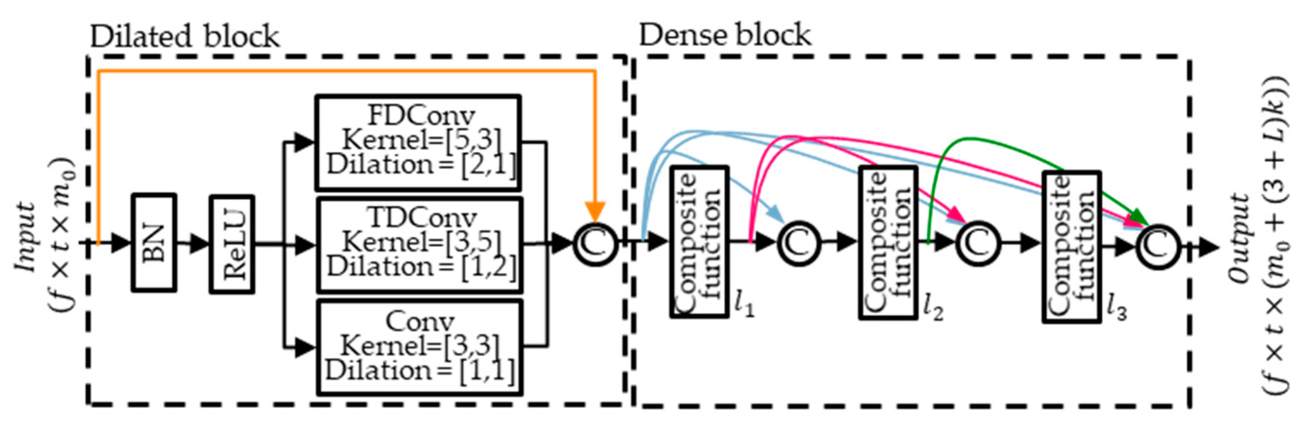
3.1. DenseNet and Dilated Dense Block

The dilated dense block architecture had the dilated block on the left and the dense block on the right, as shown in Figure 1. The dilated block can consider a wide receptive field and the dense block outputs a feature map containing more accurate target information while passing through several layers. Therefore, we placed the dense block after the dilated block in order to naturally inherit the influence considering the wide receptive field. The dense block of DenseNet concatenates the output feature maps, which is the output of the CNN filter convolving with the input data [39,40], as shown in the right block of Figure 1 in order to exploit the advantage of efficient information transmission in the feed-forward and error back-propagation processes. The dense block is composed of several composite functions [36], and the composite function consists of a sequence of batch normalization (BN) [41], rectified linear unit (ReLU) [42], and $3\times 3$ convolution (Conv). The equation below represents the concatenation of the dense block.

$$x_{\ell }=H_{\ell }\left(\left[x_0,x_1,\dots ,x_{\ell -1}\right]\right),$$

(1)

where $x_{\ell }$ represents the output of the $\ell$ layer, and $H_{\ell }$ represents the composite function. $\left[x_0,x_1,\dots ,x_{\ell -1}\right]$ indicates concatenating all the feature map from the 0 to $\ell -1$ layer.

The purpose of the dilated block is to increase the receptive field more effectively with down-sampling and up-sampling on a spectrogram. The dilated block is an architecture in which the frequency dilated convolution (FDConv), time dilated convolution (TDConv), and $3\times 3$ standard convolution are configured in parallel after BN and ReLU, as shown in the left block of Figure 1. The dilated convolution [34] was used for the FDConv and TDConv, and the kernel size and dilation rate were adjusted appropriately to the frequency and time axes, as shown in Figure 1 [33]. In the image task, the dilation rate of dilated convolution changes the horizontal and vertical axes at the same ratio because the size of the target image changes at the same ratio in width and height according to the distance [34]. However, in the spectrogram, since the acoustic characteristics of the time axis and the frequency axis changes with independent influences, the FDConv and TDConv are arranged in parallel. For example, the speech rate affects the time axis, and the gender-dependent pitch affects the frequency axis. The FDConv broadens the receptive field of the frequency axis, and the TDConv broadens the receptive field of the time axis. The dilated block is located in front of the dense block, and this whole architecture is called a dilated dense block. The number of output feature maps in the dilated block is $m_0+3k$, and the number of output feature maps in the dilated dense block is $m_0+\left(3+L\right)k$. $m_0$ is the number of input feature maps, $k$ is the growth rate, and $L$ is the number of composite functions [36].

3.2. Multi-Scale Dilated Time-Frequency DenseLSTM

MDilDenseLSTM is an architecture consisting of the dilated dense block (DDB), compression block (“Compr.”), LSTM block, down-sampling, and up-sampling, as shown in Figure 2. MDilDenseLSTM has four down-sampling (DS) and four up-sampling (US). The down-sampling used $2\times 2$ average pooling and the up-sampling used $2\times 2$ transposed convolution. The LSTM block is placed before the up-sampling, which makes scale 1 and the up-sampling located at the smallest scale. The advantage of the information and error transmission is further enhanced through an inter-block skip connection that connects outputs of the same size to each other during encoding and decoding [25]. The compression block compresses the information of many feature map into a small number of feature maps. The down-sampling and up-sampling reduces or increases the time-frequency size of the compressed feature map. The LSTM block, which is located between the compression block and up-sampling, outputs the target sequence information along the time axis. MDilDenseLSTM is a CRNN architecture by combining a CNN-based dilated dense block and an RNN-based LSTM block and is suitable when the input is an image and time series data such as a spectrogram.

The compression block [36] consists of the BN, ReLU, and $1\times 1$ convolution, and is placed behind the dilated dense block to appropriately limit the number of output feature maps from the dilated dense block and compress information at the same time. In the dilated dense block, which is a DenseNet-based architecture, since the output feature maps of each layer are concatenated, the number of output feature maps increases by the product of the number of layers. The compression rate $\theta$ has a value of $0<\theta \le 1$. The number of output feature maps by placing a compression block behind the dilated dense block can be expressed as $⎣\left(m_0+\left(3+L\right)k\right)\times \theta ⎦$, and when $\theta =1$, the number of feature maps is maintained without compression.

As shown in Figure 3, the LSTM block consists of a sequence layer of a $1\times 1$ convolution, BLSTM, and FCNN, and has an architecture in which the input feature map is concatenated to the output feature map. The LSTM block makes the CNN-based DenseNet architecture into a CRNN architecture. In the CRNN architecture, a feature is firstly extracted with the CNN, and then the RNN using time series information extracts features and classifies the input into the target class [28]. Since the feature maps obtained from the spectrogram retain the time series information as it is, adding the RNN architecture can reflect the time series information for all frames on the time axis. In addition, the receptive field can be widened on all frames of the time axis. The $1\times 1$ convolution makes the number of input feature maps to 1 and puts them into the BLSTM layer. Since the frequency dimension of the output feature map varies according to the number of nodes in the BLSTM layer, the FCNN adjusts the number of frequency dimensions in the output feature map to be the same as the number of frequency dimensions in the input feature map. Since the input feature maps and the output feature map in LSTM block are concatenated, the number of output feature maps in the dilated dense block, compression block, and LSTM block can be expressed as $⎣\left(m_0+\left(3+L\right)k\right)\times \theta ⎦+1$.

3.3. Multi-Scale Multi-Band Dilated Time-Frequency DenseLSTM

The proposed architecture, MMDilDenseLSTM, has the advantage of having a wide receptive field in the time axis as well as the frequency axis of the spectrogram by combining the dilated block designed in the previous study [33] with the MMDenseLSTM introduced in [31]. In addition, the model used in our previous study, based on a CNN architecture, had limitations in utilizing time series information in spectrograms. MMDenseLSTM extracts CNN features from dense blocks and then extracts features considering time series information from LSTM blocks. We can extract a CNN feature considering a wider range by adding a dilated block to the dense block, and then the LSTM block takes over the influence by using the CNN feature as the input. It is an architecture in which the spectrogram is divided into three bands and MDilDenseLSTM is arranged in parallel in each band and the full band, as shown in Figure 4. Since we used the audio sampled at 16 kHz as our dataset, we used a spectrogram with a frequency range of 8 kHz as input. Therefore, the frequency band was divided by the boundary of 2 kHz and 4 kHz, and the ratio was equal to that of MMDenseLSTM [31]. Moreover, 0~2 kHz is a low band, which is a frequency band where the speech signals mainly exist, 2~4 kHz is called the middle band, and 4~8 kHz is called the high band. The output of each MDilDenseLSTM is combined into one tensor, and a mask of the same size as the input is outputted through the dilated dense block, the compression block, and the last $3\times 3$ convolution.

For each MDilDenseLSTM, the growth rate and the number of composite functions in the dilated dense block, and the number of LSTM blocks were applied differently.

Table 1. Details of the proposed architecture (scale, the number of output feature map). If the bidirectional long short-term memory (BLSTM) layer was applied, the number of nodes was indicated in parentheses. The “$L$” of full band is shown in Figure 2. The lack of values indicates no architecture. Therefore, DDB and CP4 of the low band is connected to US3 and CC3. $k$: growth rate, $L$: the number of the composite function, $\theta$: compression rate, DDB: dilated dense block, CP: compression block, DS: down-sampling, US: up-sampling, CC: concatenation.

	$\mathbf{Band} (\mathit{k}$$,\mathit{L}$$,\mathit{\theta }$	Low (15, 5, 0.095)	Middle (4, 4, 0.25)	High (2, 1, 0.4)	Full (7, -, 0.2)
Layer
$3\times 3$ Conv		1, 32	1, 32	1, 32	1, 32
DDB and CP1		1, 13	1, 15	1, 16	1, 14
DS1		1/2, 13	1/2, 15	1/2, 16	1/2, 14
DDB and CP2		1/2, 11	1/2, 10	1/2, 9	1/2, 11
DS2		1/4, 11	1/4, 10	1/4, 9	1/4, 11
DDB and CP3		1/4, 11	1/4, 9	1/4, 7 (8)	1/4, 12
DS3		1/8, 11	1/8, 9	-	1/8, 12
DDB and CP4		1/8, 12 (128)	1/8, 10 (32)	-	1/8, 13
DS4		-	-	-	1/16, 13
DDB and CP5		-	-	-	1/16, 14 (128)
US4 and CC4		-	-	-	1/8, 27
DDB and CP6		-	-	-	1/8, 16
US3 and CC3		1/4, 23	1/4, 19	-	1/4, 28
DDB and CP7		1/4, 12	1/4, 11	-	1/4, 15
US2 and CC2		1/2, 23	1/2, 21	1/2, 16	1/2, 26
DDB and CP8		1/2, 13 (128)	1/2, 12	1/2, 9	1/2, 14 (128)
US1 and CC1		1, 26	1, 27	1, 25	1, 28
DDB and CP9		1, 13	1, 13	1, 13	1, 14
Concatenation		1, 27
DDB and CP10		(Parameter: $k$ = 12, $L$ = 3, $\theta$ = 0.2) 1, 19
$2\times 1$ Conv		1, 1

shows the detailed architecture of MMDilDenseLSTM. The growth rate, the number of composite functions, and the scale of each band, which are hyper-parameters of MMDilDenseLSTM, were referred to MMDenseLSTM [31]. Since the low frequency band is important due to the characteristics of the acoustic signal, the growth rate $k$ and the number $L$ of the composite function in the low band and full band, which include low frequency band, were applied more than other bands. In addition, the LSTM block in the low and full band was applied before the up-sampling, which makes scale 1 and the up-sampling located at the smallest scale. However, the LSTM block in the high and middle band was applied only before the up-sampling located at the smallest scale. In full band, since the input size is more than twice that of other bands, the receptive field must be large; therefore, the scale is lower than that of other bands. In order to combine the output feature maps along the frequency axis from each MDilDenseLSTM except for the full band, the number of output feature maps must be the same; therefore, the number of output feature maps is made the same by adjusting the compression rate applied to each band.

To learn the proposed architecture, the following loss function was used.

$$L\left(X,Y\right)=\Vert Y-X ⨀ \widehat{M}{\Vert }_1$$

(2)

where $X$ is the magnitude spectrogram of the input data, $Y$ is the magnitude spectrogram of the reference data, $⨀$ is element-wise multiplication, $\widehat{M}$ is a mask estimated by neural network, and ${\Vert .\Vert }_1$ is 1-norm. The estimated $\widehat{M}$ is multiplied by the input spectrogram $X$ to estimate clean speech data, and the difference from $Y$ is obtained by 1-norm.

4. Experiments

In order to find out how well the proposed architecture separated the music and speech signals with different characteristics, we conducted experiments for music and speech, respectively. In the speech experiment, when speech, noise, and music were mixed, clean speech signals were estimated, and then a speech recognition experiment was performed using the estimated speech signals. In the music experiment, when mixed music and speech were extracted from broadcast contents of various genres, a music signal was separated out, and then a music identification experiment was performed using the separated music signal. Section 4.1 describes the speech domain experiment, and Section 4.2 describes the music domain experiment.

4.1. Speech Experiment

4.1.1. Dataset for Speech Experiment

For the speech enhancement experiment, we mixed the music and noise signal with the speech signal. We used 115 noises database (DB) [43], ESC-50 [44], and NOISEX-92 [45] as the noise DB, WSJ1 [46] as the speech DB, and MUSDB [47] as the music DB.

The speech, music, and noise DB is organized, as shown in

Table 2. Dataset configuration for speech experiment.

DB	Noise			Music	Speech
	115 Noise	ESC-50	NOISEX-92	MUSDB	WSJ1
Training	2.3 h (165 types)		Not used	5 h (86 songs)	30 h (57 utterances $\times$ 284 speakers)
Validation	30 min (165 types)		Not used	1 h (14 songs)	5 h (35 utterances $\times$ 60 speakers)
Test	Not used		18 min (6 types)	3.5 h (50 songs)	30 min (284 utterances $\times$ 10 speakers)
Remark	Used for training and validation		Used for test	Different song for each dataset	Independent speaker for each dataset

. MUSDB is already divided into training, validation, and test datasets, and NOISEX-92 is composed of 6 noise types (babble, destroyer engine, destroyer operation, factory1, factory2, m109). WSJ1, a speech DB, is already divided into the training, validation, and test datasets. For the test dataset of speech DB, the eval93 dataset, which is the “si_et_h1” folder, in WSJ1 was used.

Since the size of the public noise DBs is small, several public noise DBs were used. To cope with various noise types, the deep learning model used 115 noise DB and ESC-50 DB with many noise types for training, while the remaining NOISEX-92 DB was used for the test. Because the public noise DB and music DB have less data than the target speech DB, they are repeatedly mixed. Since speech DB is used only once, the mixed signals are different. Of course, it would be nice if the amount of noise and music DB was as large as the speech DB, but it is not easy to collect noise and music data as much as the speech DB.

Mixed training, validation, and test datasets are created by using each training, validation, and test datasets of music, noise, and speech databases. The training data mixes the noise and music signals to have a random signal-to-noise ratio (SNR) and signal-to-music ratio (SMR) from −10 to 20 dB based on the speech signal. The validation data mixes through the same process as training. To create the test dataset for each SNR and SMR combination, the music is mixed with an SMR of −10, −5, 0, 5, 10, 20, and 30 dB, and the noise is mixed with an SNR of −10, 0, and 10 dB. As a result, the total training dataset and validation dataset were 30 h and 5 h, respectively. In addition, the test dataset for each SNR and SMR combination is 30 min.

4.1.2. Setup for Speech Experiment

We used the spectrogram magnitude of the 16 kHz single-channel audio signal as the model input. Spectrograms can be obtained through a short-time Fourier transform (STFT) with Hanning window of 320 samples and 50% overlap. The number of frames in the input spectrogram is 256. The learning rate was 0.001 and the optimizer used Adam [48]. The batch size was 16 and the number of epochs was 20. The validation dataset was tested at every epoch and the model with the best signal-to-distortion ratio (SDR) [49] was finally selected and tested. To evaluate speech enhancement performance, we performed a subjective speech quality test. In addition, we also calculated objective measures. As objective measures, SDR, which is the signal separation performance, and perceptual evaluation of speech quality (PESQ) [50], which is performance related to speech quality, and short-time objective intelligibility (STOI) [51], normalized-covariance measure (NCM) [52], coherence-based speech intelligibility index (CSII) [53], which are speech intelligibility measures, were computed. PESQ ranges from −0.5 to 4.5, STOI, NCM, and CSII range from 0 to 1, and SDR had no fixed range. Larger values of the performance evaluation indicators represented better performance. In addition, to evaluate speech recognition performance, we used the nnet3 (chain) model of the Kaldi toolkit [54]. The Kaldi speech recognition model was trained with the WSJ1’s clean speech, the SI-284 training dataset. The speech recognition performance is computed by word error rate (WER), and lower WER indicates better performance.

4.1.3. Experimental Results of the Subjective Quality Measure for Speech Enhancement

We tested four models for speech enhancement: GRN [35], MMDenseLSTM [31], DilDenseNet [33], and the proposed architecture. In several recent studies [55,56], GRN proposed for speech enhancement was experimented for performance comparison. Deep learning models were implemented by ourselves because there was no open code. In DilDenseNet which we designed in the previous experiment [33], we did not reverse the feature map in the multi-band block for speech enhancement and deleted the multi-band block in the decoding process. In addition, dividing the band at 2 kHz and 4 kHz was equally applied to DilDenseNet, MMDenseLSTM, and proposed architecture. It was confirmed by experiments that these modifications showed better performance in speech enhancement.

For the subjective listening evaluation of the speech quality, we conducted a relative preference test [57] targeting GRN, MMDenseLSTM, DilDenseNet, and the proposed architecture. From the four models, we obtained six combinations of model for comparison. The subjects participated in a total of 18 conditions (six combinations of model for comparison, three different noise and music levels). Each condition had five pairwise comparisons and the subject performed a total of 90 pairwise comparisons. To prevent subjects from predicting information, such as the condition and speech material of each sample, we provided the condition and speech material in random order, and the sample length used for each preference test was 2–3 s. In addition, each subject independently conducted the subjective evaluation in order not to share their opinions with each other. In each pairwise comparison, a mixture and pairs of enhanced speech samples, which resulted from the comparison models, were provided, and the mixture was always heard first.

As a total of 30 subjects participated in the subjective listening test, 150 preference results were obtained for each condition. The listeners had the ability to select a preferred sample (1 score) or “can’t decide” (0.5 score), and the preference score and significance were calculated by combining the preference results of all listeners. We determined the preference score by applying the average to the preferred frequency. In addition, we calculated the one-tailed significance of the binomial test.

Table 3. Result of subjective listening test. “Hard” indicates an environment that music and noise are mixed at 0 dB, “Medium” mixed at 5 dB, and “Easy” mixed at 10 dB (“n.s.”: not significant, “$*$”: p < 0.05, “$**$”: p < 0.01, “$***$”: p < 0.001).

	Environment	Hard	Medium	Easy	Total
Model Comparison
Proposed > DilDenseNet		0.60 ($**$)	0.60 ($*$)	0.59 ($*$)	0.60 ($***$)
Proposed > MMDenseLSTM		0.61 ($**$)	0.67 ($***$)	0.62 ($**$)	0.63 ($***$)
Proposed > GRN		0.89 ($***$)	0.79 ($***$)	0.71 ($***$)	0.80 ($***$)
DilDenseNet > MMDenseLSTM		0.57 (n.s.)	0.51 (n.s.)	0.42 (n.s.)	0.50 (n.s.)
DilDenseNet > GRN		0.79 ($***$)	0.79 ($***$)	0.68 ($***$)	0.76 ($***$)
MMDenseLSTM > GRN		0.88 ($***$)	0.82 ($***$)	0.88 ($***$)	0.86 ($***$)

shows the preference scores of the subjective speech quality listening test for the proposed architecture and other deep learning architectures. In the subjective evaluation, the speech quality of the proposed architecture was evaluated better than DilDenseNet, MMDenseLSTM, and GRN. DilDenseNet and MMDenseLSTM were evaluated to have the same speech quality. GRN was evaluated to have the lowest speech quality among deep learning architectures. In addition, the comparisons including GRN showed high significance in all conditions, which indicated that the difference in performance from other deep learning structures was clear. Likewise, “Total” results of all comparisons other than the DilDenseNet and MMDenseLSTM comparisons showed high significance and thus represent reliable results.

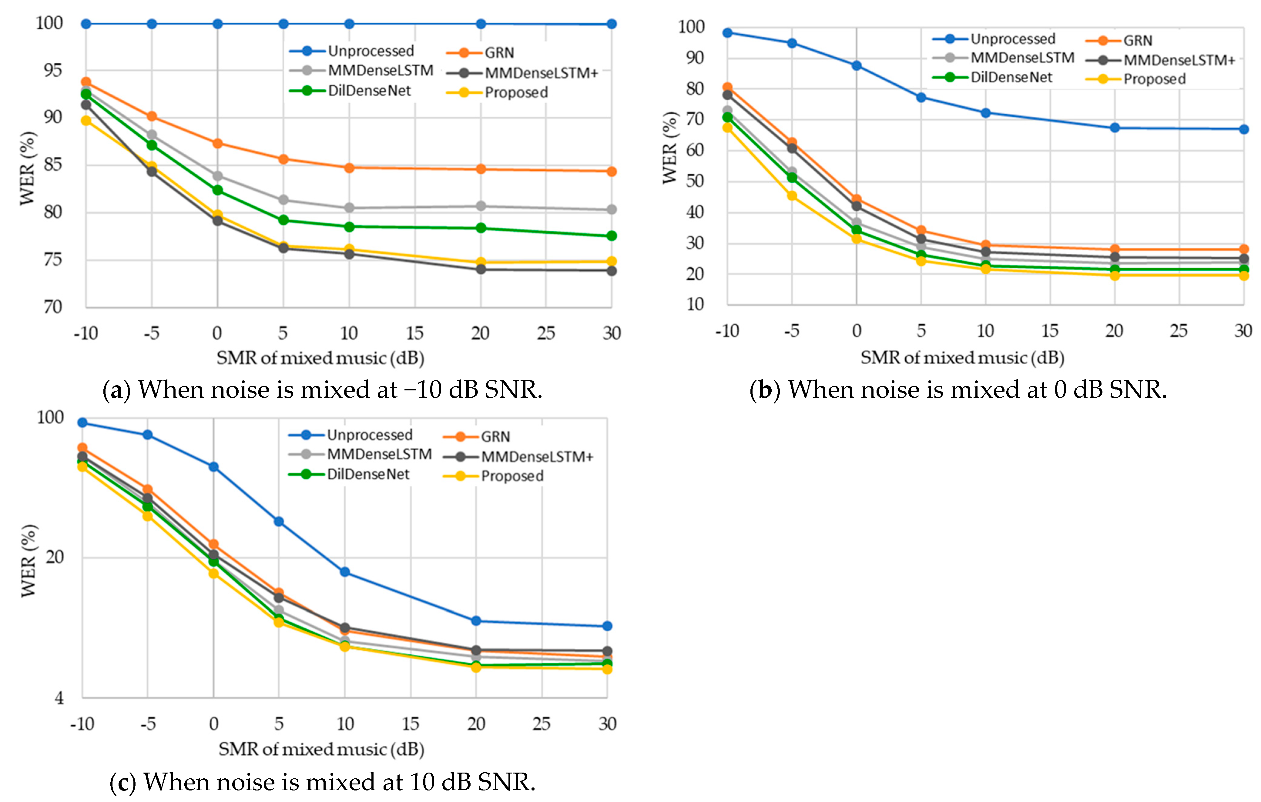
4.1.4. Experimental Results of the Objective Measures for Speech Enhancement and Recognition

In speech recognition after speech enhancement, objective indicators (PESQ, SDR, STOI, NCM, SCII, and WER) were measured for GRN, MMDenseLSTM, DilDenseNet, proposed architecture, and MMDenseLSTM+, which increased only the number of parameters in MMDenseLSTM.

Table 4. Number of parameters for each architecture in this experiment.

Architecture	$\mathbf{The} \mathbf{Number} \mathbf{of} \mathbf{Parameters} (\times {10}^6)$
GRN	3.11
MMDenseLSTM	0.98
MMDenseLSTM+	1.51
DilDenseNet	0.47
Proposed	1.49

shows the number of parameters for each architecture. The proposed architecture had 50% more parameters than MMDenseLSTM because it is an architecture in which dilated blocks are added to MMDenseLSTM. Since the performance may be improved simply by increasing the parameters of MMDenseLSTM, we designed MMDenseLSTM+ having almost the same number of parameters as the proposed architecture to confirm this. MMDenseLSTM+ has the same architecture as MMDenseLSTM, and the hyper-parameter (growth rate, compression rate, the number of composite function) was properly adjusted.

Figure 5 compares the results of PESQ, SDR, STOI, NCM, SCII, and WER for each deep learning architecture and an unprocessed mixture signal in 0 dB SMR and SNR environments. MMDenseLSTM+ showed the best performance among the deep learning architectures in SDR results and showed the same or better performance than MMDenseLSTM in PESQ, STOI, and CSII, but showed lower NCM, WER performance than MMDenseLSTM, DilDenseNet, and the proposed architecture. Therefore, we can see that simply increasing the parameter did not improve the performance. In addition, GRN had more than twice the parameters of the proposed architecture but showed the lowest performance among deep learning architectures. Lastly, the proposed architecture showed lower performance than MMDenseLSTM and MMDenseLSTM+ in SDR, but it had the best performance in other results. In particular, the proposed architecture in WER showed a relatively 14.4% improvement in performance compared to MMDenseLSTM, and it showed the best performance compared to other deep learning architectures. Overall, PESQ, STOI, CSII, and NCM performance showed a higher correlation with WER results than SDR performance, and especially NCM had the highest correlation. The matched pairs sentence-segment word error test [58] using the NIST speech recognition scoring toolkit (SCTK) (https://github.com/usnistgov/SCTK) was performed to confirm the statistical significance in the WER results of Figure 5. In the comparison between the proposed architecture and DilDenseNet, the p-value was less than 0.01, and in the comparison between the proposed architecture and other deep learning architectures, the p-value was less than 0.001 in all cases. Therefore, in the WER results of Figure 5, the difference in performance between the proposed architecture and other deep learning architectures was statistically significant.

Figure 6 shows the speech recognition results for the unprocessed mixture signal and signals enhanced by the deep learning models. Figure 6a–c show the WER results with SNR of −10, 0, and 10 dB, respectively. In Figure 6a, MMDenseLSTM+ shows the best performance. However, Figure 6b,c shows how the performance of MMDenseLSTM+ deteriorated more and more in an environment with higher SNR. GRN showed the lower overall performance than others, and then MMDenseLSTM and DilDenseNet showed good performance in order. The proposed architecture showed the best performance after MMDenseLSTM+ at −10 dB SNR, but the difference of performance from MMDenseLSTM+ was not large, and it showed the best performance in 0 dB and 10 dB SNR environments, as can be seen in

Table 5. Average word error rate (WER) over the entire signal-to-music ratio (SMR) at each signal-to-noise ratio (SNR). Lower WER indicates better performance.

	SNR	−10	0	10
Architecture
GRN		87.26	44.04	24.89
MMDenseLSTM		84.01	37.79	21.91
MMDenseLSTM+		79.24	41.51	23.01
DilDenseNet		82.26	35.54	20.77
Proposed		79.55	32.83	19.20

.

4.2. Music Experiment

We experimented with the proposed architecture in the previous task [33]. Figure 7 shows the overall structure of the music experiment. The mixture of music and speech was separated into a clean music signal in the music separation model, and music identification was attempted using the separated music signal. Speech collected from broadcast contents were mixed with music at −30~0 dB music-to-speech ratio (MSR), and then the mixed signal was used as the input and the music signal was used as the target to train the music separation model.

Fingerprints were extracted from all the songs used for evaluation and then stored in the fingerprint database. The fingerprint of the separated music signal was extracted and matched with all the songs in the fingerprint database to find matching music. For the fingerprint, the landmark-based audio fingerprinting method [59] was used. The landmark-based fingerprint was created by first extracting peak points from the spectrogram of the query sample in consideration of density and then connecting the peak points [59]. It will be an important point to determine the music identification performance that the peak points of the estimated music signal are well preserved. In addition, in a deep learning model that divides the frequency band of the spectrogram, it is necessary to examine how the boundary of the frequency band affects the fingerprint.

4.2.1. Dataset for Music Experiment

Table 6. Dataset configuration for music experiment. The sample length is 12 s.

DB	Music	Speech	Remark
Training	extracted 1 sample in each song (1673 songs, 5 h 30 min)	1673 samples (5 h 30 min)	Used for the training and validation of the separation model
Validation	extracted 1 sample in each song (150 songs, 30 min)	150 samples (30 min)
Test	extracted 2 samples in each song (7295 songs, 48 h)	1823 samples (6 h)	Used for measuring the separation and identification performances
All	9118 songs	3646 samples

shows the configuration of training, validation, and test datasets for the music experiment. The music DB had 9118 popular songs from various countries and genres. The speech DB had 12 h of broadcast contents of various genres (drama, entertainment, documentary, and kids). The training data were mixed at a random MSR between −30 and 0 dB, considering the characteristics of broadcast content in which the speech signal was mixed in a larger volume than the music signal. Test data were mixed at −10 dB, 0 dB MSR. There were 14,590 query samples per MSR case. When creating the training and test dataset, the speech was randomly selected and mixed with the music because the speech data was smaller than the music data. Both speech and music data were recorded with 44,100 Hz sampling.

4.2.2. Setup for Music Experiment

We used a mono signal down-sampled to 16 kHz for the experiment. The input of the deep learning architectures is a spectrogram using 1024-point STFT with Hanning window and 75% overlap size. The spectrogram estimated from the deep learning algorithm was reconstructed as a waveform and used as an input for the identification program. For music identification, the landmark-based identification program (https://github.com/dpwe/audfprint) was used. For the Wave-U-Net architecture, we used the open-source (https://github.com/f90/Wave-U-Net) that the author provided. Other deep learning architectures were implemented directly for the experiment by ourselves.

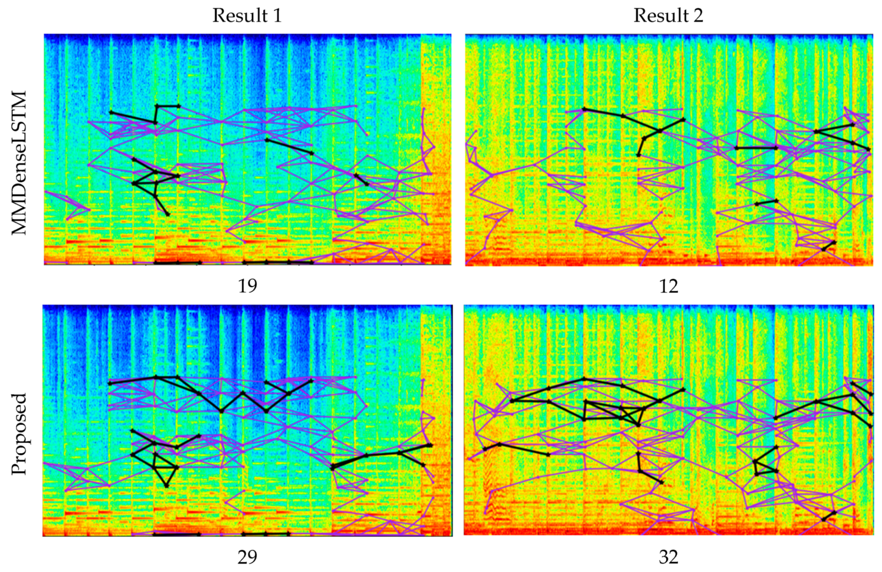
4.2.3. Experimental Results for Music Signal Separation and Identification

In order to compare the objective performance differences of deep learning architectures, we performed music signal separation and music identification experiments of several deep learning architectures in the same environment. The separation performance was SDR and was expressed using median and mean statistics. The music identification performance was the identification accuracy. The performance of other deep learning architectures except the proposed architecture was the same as the previous study [33]. In addition, we analyzed the fingerprint used in the music identification system. Since the fingerprint was composed of indexes, it could be plotted overlapped on the spectrogram, which helped intuitive interpretation.

Table 7. Music separation performance measured in signal-to-distortion ratio (SDR) (dB) on broadcast contents. MSR: music-to-speech ratio.

Architecture	0 dB MSR		−10 dB MSR
	Median SDR	Mean SDR	Median SDR	Mean SDR
U-Net	6.24	6.19	3.18	3.11
Wave-U-Net	6.33	6.22	2.97	2.86
MDenseNet	6.98	6.86	3.84	3.67
MMDenseNet	7.15	7.10	4.04	3.91
MMDenseLSTM	7.40	7.38	4.13	4.05
DilDenseNet	7.72	7.63	4.44	4.32
Proposed	7.69	7.65	4.54	4.40

shows the separation performance. The proposed architecture improved the separation performance of MMDenseLSTM, and it showed the best performance compared to other deep learning architectures.

Table 8. MI accuracy (%) and the average number of matched fingerprints ($MF$) in the identified queries.

Architecture	0 dB MSR		−10 dB MSR
	MI Accuracy	$\mathit{M}\mathit{F}$	MI Accuracy	$\mathit{M}\mathit{F}$
Unprocessed	43.38	20.2	4.59	11.8
U-Net	42.33	16.0	19.38	11.8
Wave-U-Net	54.77	19.1	26.89	12.4
MDenseNet	52.57	19.1	28.44	13.2
MMDenseNet	49.66	17.4	26.67	12.3
MMDenseLSTM	67.94	22.0	44.96	14.9
DilDenseNet	71.91	23.8	48.03	15.5
Proposed	73.35	25.0	50.75	16.1
Oracle	95.92	72.6	95.92	72.6

shows the music identification (MI) performance and the average number of matched fingerprints ($MF$) in the identified queries. Likewise, the proposed architecture in which the dilated block was added to MMDenseLSTM improved the identification performance of MMDenseLSTM by 16.9% at 0 dB MSR and 10.5% at −10 dB MSR, relatively, and it showed the best performance compared to the existing deep learning architecture. The statistical significance test was confirmed through the SCTK toolkit in the MI results of Table 8. The proposed architecture showed the p-value less than 0.001 in all comparisons with other deep learning architectures. In the 0 dB, −10 dB MSR environment, the difference in performance between the proposed architecture and other deep learning architectures was statistically significant. Apart from the identification performance, $MF$ showed how well the peaks were estimated. Overall, $MF$ has correlation with the identification performance. However, at 0 dB MSR, the $MF$ for the unprocessed signal was quite high considering the identification performance. This showed that the landmark-based fingerprinting scheme was robust to noise at 0 dB MSR. The proposed architecture showed the largest $MF$ except Oracle at 0 dB and −10 dB MSR.

Figure 8 shows the fingerprints of the separated music signal from the MMDenseLSTM and the proposed architecture. In both results, the proposed architecture had a larger number of matched fingerprints than the MMDenseLSTM. This means that the peak points of the estimated music signal were better preserved in the proposed architecture than in MMDenseLSTM. In Result 1, the matched fingerprints of the low band were the same in the MMDenseLSTM and the proposed architecture, and more fingerprints were matched in the middle and high bands of the proposed architecture. In Result 2, the proposed architecture showed more matched fingerprints in wider areas of the middle and high bands than the MMDenseLSTM.

In the previous study, we found that distortion occurs at the frequency band boundary of the output spectrogram when the deep learning architecture was designed by independently placing excessive parameters in each frequency band of the input spectrogram [33]. We investigate whether such distortion interferes with fingerprint extraction and how much such distortion occurs in each deep learning architecture as the quantitative indicator. To express the effect of this distortion as the quantitative indicator, the average number of all fingerprints across the frequency boundaries ($AcrAF$) and the average number of matched fingerprints across the frequency boundaries ($AcrMF$) were measured as shown in

Table 9. The average number of all fingerprints across the frequency boundaries ($AcrAF$) and the average number of matched fingerprints across the frequency boundaries ($AcrMF$).

Architecture	0 dB MSR		−10 dB MSR
	$$\mathit{A}\mathit{c}\mathit{r}\mathit{A}\mathit{F}$$	$$\mathit{A}\mathit{c}\mathit{r}\mathit{M}\mathit{F}$$	$$\mathit{A}\mathit{c}\mathit{r}\mathit{A}\mathit{F}$$	$$\mathit{A}\mathit{c}\mathit{r}\mathit{M}\mathit{F}$$
Unprocessed	32.0	2.9	27.0	1.6
U-Net	29.7	2.1	25.1	1.6
Wave-U-Net	33.7	2.6	30.4	1.7
MDenseNet	25.7	2.6	21.6	1.8
MMDenseNet	23.7	2.0	20.1	1.5
MMDenseLSTM	31.0	2.9	26.4	1.9
DilDenseNet	30.3	3.1	25.8	2.0
Proposed	30.7	3.3	26.6	2.1
Oracle	33.6	9.5	33.6	9.5

. In our experiment, deep learning architectures in which many parameters were placed independently in each frequency band were MMDenseNet, MMDenseLSTM, and the proposed architecture, and the frequency band boundaries were 2 and 4 kHz. MMDenseNet had the smallest value in these two indicators, which could explain why MMDenseNet showed higher separation performance than Wave-U-Net and MDenseNet but had lower music identification performance. In the identification performance, $AcrMF$ represented matched fingerprints and was more important than $AcrAF$ index. Which represented all fingerprints. The proposed architecture had more $AcrMF$ value than other deep learning architectures.

5. Conclusions

We proposed an MMDilDenseLSTM for speech recognition or music identification after audio source separation. MMDilDenseLSTM is a CRNN-based MMDenseLSTM and it has a dilated block that effectively increases the receptive field in consideration of acoustic characteristics in the spectrogram.

In the speech recognition experiment after speech enhancement, subjective evaluation was performed on the enhanced speech, and various objective indicators (PESQ, SDR, STOI, CSII, NCM, and WER) were measured. Encoder-decoder style architectures, MMDenseLSTM, DilDenseNet, and the proposed architecture showed better performance with fewer parameters than GRN. In addition, it was confirmed that simply increasing the number of parameters did not improve performance. The speech recognition performance of WER had a highest correlation with NCM than with other indicators, and the proposed architecture in the preference score, PESQ, STOI, CSII, NCM, and WER showed the best performance compared to other deep learning architectures.

In the music identification experiment after music signal separation, the performance of separation was measured using SDR. Although SDR and identification accuracy did not have a correlation in all deep learning architectures, the proposed architecture showed the best performance compared to other deep learning architectures in SDR performance and identification performance. In addition, when the fingerprints of the query and reference were plotted overlapped, it was confirmed that more fingerprints are matched over wider areas in the proposed architecture than in the MMDenseLSTM.

In conclusion, the proposed architecture greatly improved the performance of MMDenseLSTM in all experiments for speech and music signals, and it showed the best performance compared to other deep learning architectures. In addition, it was shown that the separation performance was not quite well correlated with the overall system performance. When determining the architecture of the separation model, the characteristics of the system to which the separated signal was to be applied should be taken in consideration. Based on these results, we expected that the proposed architecture could be successfully applied to music identification and speech recognition systems in noisy environments, e.g., speech recognition in cars or automatic music identification in stores. However, there were clear limitations in deep learning models operating in the spectrum domain as in our proposed method because the phase information of the mixture causes distortion in the signal restoration process. In future work, we plan to alleviate this problem by taking a model operating in the waveform domain as baseline.

References

1. Bregman, A.S. Auditory Scene Analysis: The Perceptual Organization of Sound; The MIT Press: Cambridge, MA, USA, 1990. [Google Scholar]
2. Hirsch, H.G.; Ehrlicher, C. Noise estimation techniques for robust speech recognition. In Proceedings of the IEEE International Conference on Acoustics, Speech, and Signal Processing (ICASSP), Detroit, MI, USA, 9–12 May 1995; Volume 1, pp. 153–156. [Google Scholar]
3. Zhang, H.; Liu, C.; Inoue, N.; Shinoda, K. Multi-task autoencoder for noise-robust speech recognition. In Proceedings of the IEEE International Conference on Acoustics, Speech, and Signal Processing (ICASSP), Calgary, AB, Canada, 15–20 April 2018; pp. 5599–5603. [Google Scholar]
4. Lee, D.D.; Seung, H.S. Learning the parts of objects by non-negative matrix factorization. Nature 1999, 401, 788–791. [Google Scholar] [CrossRef]
5. Fan, H.T.; Hung, J.; Lu, X.; Wang, S.S.; Tsao, Y. Speech enhancement using segmental nonnegative matrix factorization. In Proceedings of the IEEE International Conference on Acoustics, Speech, and Signal Processing (ICASSP), Florence, Italy, 4–9 May 2014; pp. 4483–4487. [Google Scholar]
6. Sprechmann, P.; Bronstein, A.M.; Sapiro, G. Supervised non-Euclidean sparse NMF via bilevel optimization with applications to speech enhancement. In Proceedings of the Joint Workshop on Hands-free Speech Communication and Microphone Arrays (HSCMA), Nancy, France, 12–14 May 2014; pp. 11–15. [Google Scholar]
7. Vincent, E.; Bertin, N.; Gribonval, R.; Bimbot, F. From blind to guided audio source separation: How models and side information can improve the separation of sound. IEEE Signal Process. Mag. 2014, 31, 107–115. [Google Scholar] [CrossRef] [Green Version]
8. Wang, Y.; Wang, D. Towards scaling up classification-based speech separation. IEEE Trans. Audio Speech Lang. Process. 2013, 21, 1381–1390. [Google Scholar]
9. Xu, Y.; Du, J.; Dai, L.-R.; Lee, C.-H. An experimental study on speech enhancement based on deep neural networks. IEEE Signal Process. Lett. 2014, 21, 65–68. [Google Scholar] [CrossRef]
10. Kang, T.G.; Kwon, K.; Shin, J.W.; Kim, N.S. NMF-based target source separation using deep neural network. IEEE Signal Process. Lett. 2015, 22, 229–233. [Google Scholar] [CrossRef]
11. Grais, E.; Sen, M.; Erdogan, H. Deep neural networks for single channel source separation. In Proceedings of the IEEE International Conference on Acoustics, Speech, and Signal Processing (ICASSP), Florence, Italy, 4–9 May 2014; pp. 3734–3738. [Google Scholar]
12. Nugraha, A.A.; Liutkus, A.; Vincent, E. Multichannel music separation with deep neural networks. In Proceedings of the European Signal Processing Conference (EUSIPCO), Budapest, Hungary, 29 August–2 September 2015; pp. 1748–1752. [Google Scholar]
13. Uhlich, S.; Giron, F.; Mitsufuji, Y. Deep neural network based instrument extraction from music. In Proceedings of the IEEE International Conference on Acoustics, Speech, and Signal Processing (ICASSP), Brisbane, Australia, 19–24 April 2015; pp. 2135–2139. [Google Scholar]
14. Le Roux, J.; Hershey, J.; Weninger, F. Deep NMF for speech separation. In Proceedings of the IEEE International Conference on Acoustics, Speech, and Signal Processing (ICASSP), Brisbane, Australia, 19–24 April 2015; pp. 66–70. [Google Scholar]
15. Hsu, K.Y.; Li, H.Y.; Psaltis, D. Holographic implementation of a fully connected neural network. Proc. IEEE 1990, 78, 1637–1645. [Google Scholar] [CrossRef]
16. LeCun, Y.; Bottou, L.; Bengio, Y.; Haffner, P. Gradient-based learning applied to document recognition. Proc. IEEE 1998, 86, 2278–2324. [Google Scholar] [CrossRef] [Green Version]
17. Werbos, P.J. Backpropagation through time: What it does and how to do it. Proc. IEEE 1990, 78, 1550–1560. [Google Scholar] [CrossRef] [Green Version]
18. Chen, J.; Wang, D. Long short-term memory for speaker generalization in supervised speech separation. J. Acoust. Soc. Am. 2017, 141, 4705–4714. [Google Scholar] [CrossRef]
19. Weninger, F.; Eyben, F.; Schuller, B. Single-channel speech separation with memory-enhanced recurrent neural networks. In Proceedings of the IEEE International Conference on Acoustics, Speech, and Signal Processing (ICASSP), Florence, Italy, 4–9 May 2014; pp. 3709–3713. [Google Scholar]
20. Fu, S.-W.; Tsao, Y.; Lu, X. SNR-aware convolutional neural network modeling for speech enhancement. In Proceedings of the INTERSPEECH, San Francisco, CA, USA, 8–12 September 2016; pp. 3768–3772. [Google Scholar]
21. Kounovsky, T.; Malek, J. Single channel speech enhancement using convolutional neural network. In Proceedings of the IEEE International Workshop of Electronics, Control, Measurement, Signals and their Application to Mechatronics (ECMSM), San Sebastian, Spain, 24–26 May 2017; pp. 1–5. [Google Scholar]
22. Uhlich, S.; Porcu, M.; Giron, F.; Enenkl, M.; Kemp, T.; Takahashi, N.; Mitsufuji, Y. Improving music source separation based on deep neural networks through data augmentation and network blending. In Proceedings of the IEEE International Conference on Acoustics, Speech, and Signal Processing (ICASSP), New Orleans, LA, USA, 5–9 March 2017; pp. 261–265. [Google Scholar]
23. Jansson, A.; Humphrey, E.; Montecchio, N.; Bittner, R.; Kumar, A.; Weyde, T. Singing voice separation with deep U-Net convolutional networks. In Proceedings of the International Society for Music Information Retrieval Conference (ISMIR), Montreal, QC, Canada, 4–8 November 2017; pp. 745–751. [Google Scholar]
24. Park, S.; Kim, T.; Lee, K.; Kwak, N. Music source separation using stacked hourglass networks. In Proceedings of the International Society for Music Information Retrieval Conference (ISMIR), Paris, France, 23–27 September 2018; pp. 289–296. [Google Scholar]
25. Takahashi, N.; Mitsufuji, Y. Multi-scale multi-band DenseNets for audio source separation. In Proceedings of the IEEE Workshop on Applications of Signal Processing to Audio and Acoustics (WASPAA), New Paltz, NY, USA, 15–18 October 2017; pp. 21–25. [Google Scholar]
26. Hochreiter, S.; Schmidhuber, J. Long short-term memory. Neural Comput. 1997, 9, 1735–1780. [Google Scholar] [CrossRef]
27. Graves, A.; Schmidhuber, J. Framewise phoneme classification with bidirectional LSTM networks. In Proceedings of the IEEE International Joint Conference on Neural Networks, Montreal, QC, Canada, 31 July–4 August 2005; Volume 4, pp. 2047–2052. [Google Scholar]
28. Shi, B.; Bai, X.; Yao, C. An end-to-end trainable neural network for image-based sequence recognition and its application to scene text recognition. IEEE Trans. Pattern Anal. Mach. Intell. 2016, 39, 2298–2304. [Google Scholar] [CrossRef] [Green Version]
29. Li, A.; Yuan, M.; Zheng, C.; Li, X. Speech enhancement using progressive learning-based convolutional recurrent neural network. Appl. Acoust. 2020, 166, 107347. [Google Scholar] [CrossRef]
30. Chakrabarty, S.; Habets, E.A.P. Time–frequency masking based online multi-channel speech enhancement with convolutional recurrent neural networks. IEEE J. Sel. Top. Signal Process. 2019, 13, 787–799. [Google Scholar] [CrossRef]
31. Takahashi, N.; Goswami, N.; Mitsufuji, Y. MMDenseLSTM: An efficient combination of convolutional and recurrent neural networks for audio source separation. In Proceedings of the International Workshop on Acoustic Signal Enhancement (IWAENC), Tokyo, Japan, 17–20 September 2018; pp. 106–110. [Google Scholar]
32. Hubel, D.H.; Wiesel, T.N. Receptive fields, binocular interaction and functional architecture in the cat’s visual cortex. J. Physiol. 1962, 160, 106–154. [Google Scholar] [CrossRef]
33. Heo, W.-H.; Kim, H.; Kwon, O.-W. Source separation using dilated time-frequency DenseNet for music identification in broadcast contents. Appl. Sci. 2020, 10, 1727. [Google Scholar] [CrossRef] [Green Version]
34. Yu, F.; Koltun, V. Multi-scale context aggregation by dilated convolutions. In Proceedings of the International Conference on Learning Representations (ICLR), San Juan, PR, USA, 2–4 May 2016. [Google Scholar]
35. Tan, K.; Chen, J.; Wang, D. Gated residual networks with dilated convolutions for monaural speech enhancement. IEEE Trans. Audio Speech Lang. Process. 2019, 27, 189–198. [Google Scholar] [CrossRef]
36. Huang, G.; Liu, Z.; Weinberger, K.Q.; Maaten, L. Densely connected convolutional networks. In Proceedings of the IEEE Conference on Computer Vision and Pattern Recognition (CVPR), Honolulu, HI, USA, 24–30 June 2017; pp. 4700–4708. [Google Scholar]
37. Stoller, D.; Ewert, S.; Dixon, S. Wave-U-Net: A multi-scale neural network for end-to-end audio source separation. arXiv 2018, arXiv:1806.03185. [Google Scholar]
38. Luo, Y.; Mesgarani, N. Conv-TasNet: Surpassing ideal time–frequency magnitude masking for speech separation. IEEE/ACM Trans. Audio Speech Lang. Process. 2019, 27, 1256–1266. [Google Scholar] [CrossRef] [Green Version]
39. Ciaburro, G. Sound event detection in underground parking garage using convolutional neural network. Big Data Cogn. Comput. 2020, 4, 20. [Google Scholar] [CrossRef]
40. Ciaburro, G.; Iannace, G. Improving smart cities safety using sound events detection based on deep neural network algorithms. Informatics 2020, 7, 23. [Google Scholar] [CrossRef]
41. Ioffe, S.; Szegedy, C. Batch normalization: Accelerating deep network training by reducing internal covariate shift. In Proceedings of the International Conference on Machine Learning (ICML), Lille, France, 6–11 July 2015; pp. 448–456. [Google Scholar]
42. Glorot, X.; Bordes, A.; Bengio, Y. Deep sparse rectifier neural networks. In Proceedings of the International Conference on Artificial Intelligence and Statistics (AISTATS), Fort Lauderdale, FL, USA, 11–13 April 2011; pp. 315–323. [Google Scholar]
43. Xu, Y.; Du, J.; Huang, Z.; Dai, L.-R.; Lee, C.-H. Multi-objective learning and mask-based post-processing for deep neural network based speech enhancement. In Proceedings of the INTERSPEECH, Dresden, Germany, 6–10 September 2015; pp. 1508–1512. [Google Scholar]
44. Piczak, K.J. ESC: Dataset for environmental sound classification. In Proceedings of the ACM International Conference on Multimedia, New York, NY, USA, 12–16 October 2015; pp. 1015–1018. [Google Scholar]
45. Varga, A.; Steeneken, H.J.M. Assessment for automatic speech recognition: II. NOISEX-92: A database and an experiment to study the effect of additive noise on speech recognition systems. Speech Commun. 1993, 12, 247–251. [Google Scholar] [CrossRef]
46. CSR-II (WSJ1) Complete. Available online: https://catalog.ldc.upenn.edu/LDC94S13A (accessed on 23 July 2020).
47. The MUSDB18 Corpus for Music Separation. Available online: https://doi.org/10.5281/zenodo.1117372 (accessed on 28 August 2020).
48. Kingma, D.; Ba, J. Adam: A method for Stochastic Optimization. In Proceedings of the International Conference on Learning Representations, San Diego, CA, USA, 7–9 May 2015. [Google Scholar]
49. Vincent, E.; Gribonval, R.; Fevotte, C. Performance measurement in blind audio source separation. IEEE Trans. Audio Speech Lang. Process. 2006, 14, 1462–1469. [Google Scholar] [CrossRef] [Green Version]
50. Rix, A.; Beerends, J.; Hollier, M.; Hekstra, A. Perceptual evaluation of speech quality (PESQ)-a new method for speech quality assessment of telephone networks and codecs. In Proceedings of the IEEE International Conference on Acoustics, Speech, and Signal Processing (ICASSP), Salt Lake City, UT, USA, 7–11 May 2001; pp. 749–752. [Google Scholar]
51. Taal, C.; Hendriks, R.; Heusdens, R.; Jensen, J. An algorithm for intelligibility prediction of time-frequency weighted noisy speech. IEEE Trans. Audio Speech Lang. Process. 2011, 19, 2125–2136. [Google Scholar] [CrossRef]
52. Ma, J.; Hu, Y.; Loizou, P.C. Objective measures for predicting speech intelligibility in noisy conditions based on new band-importance functions. J. Acoust. Soc. Am. 2009, 125, 3387–3405. [Google Scholar] [CrossRef] [Green Version]
53. Kates, J.M.; Arehart, K.H. Coherence and the speech intelligibility index. J. Acoust. Soc. Am. 2005, 117, 2224–2237. [Google Scholar] [CrossRef]
54. Povey, D.; Ghoshal, A.; Boulianne, G.; Burget, L.; Glembek, O.; Goel, N.; Hannemann, M.; Motlicek, P.; Qian, Y.; Schwarz, P.; et al. The Kaldi speech recognition toolkit. In Proceedings of the IEEE Workshop on Automatic Speech Recognition and Understanding (ASRU), Waikoloa, HI, USA, 11–15 December 2011. [Google Scholar]
55. Pirhosseinloo, S.; Brumberg, J.S. Monaural speech enhancement with dilated convolutions. In Proceedings of the INTERSPEECH, Graz, Austria, 15–19 September 2019; pp. 3143–3147. [Google Scholar]
56. Wang, P.; Wang, D. Enhanced spectral features for distortion-independent acoustic modeling. In Proceedings of the INTERSPEECH, Graz, Austria, 15–19 September 2019; pp. 476–480. [Google Scholar]
57. Choi, H.S.; Kim, J.H.; Huh, J.; Kim, A.; Ha, J.W.; Lee, K. Phase-aware speech enhancement with deep complex u-net. In Proceedings of the International Conference on Learning Representations, Vancouver, BC, Canada, 30 April–3 May 2018. [Google Scholar]
58. Gillick, L.; Cox, S.J. Some statistical issues in the comparison of speech recognition algorithms. In Proceedings of the IEEE International Conference on Acoustics, Speech and Signal Processing (ICASSP), Glasgow, UK, 23–26 May 1989; pp. 532–535. [Google Scholar]
59. Wang, A. An industrial strength audio search algorithm. In Proceedings of the International Society for Music Information Retrieval Conference (ISMIR), Baltimore, MD, USA, 26–30 October 2003; pp. 7–13. [Google Scholar]
Figure 1. The architecture of dilated dense block. The [frequency, time] denotes the kernel size and dilation rate. BN: batch normalization, ReLU: rectified linear unit, FDConv: frequency dilated convolution, TDConv: time dilated convolution.
Applsci 11 00789 g001
Figure 2. The architecture of multi-scale dilated time-frequency DenseNet with LSTM (MDilDenseLSTM). This architecture is in the full band of multi-band MDilDenseLSTM (MMDilDenseLSTM). The red dashed box represents the recurrent neural network (RNN)-based architecture. DDB: dilated dense block, LSTM: long short-term memory.
Applsci 11 00789 g002
Figure 3. The architecture of LSTM block.
Applsci 11 00789 g003
Figure 4. Proposed architecture for speech enhancement.
Applsci 11 00789 g004
Figure 5. Comparison of perceptual evaluation of speech quality (PESQ), signal-to-distortion ratio (SDR), short-time objective intelligibility (STOI), coherence-based speech intelligibility index (CSII), normalized-covariance measure (NCM), and word error rate (WER) results when the music and noise are mixed at 0 dB. PESQ, SDR, STOI, CSII, and NCM are calculated using average statistics. PESQ ranges from −0.5 to 4.5, STOI, NCM, and CSII range from 0 to 1, and SDR has no fixed range. Larger values of the performance evaluation indicators represent better performance.
Applsci 11 00789 g005
Figure 6. Speech recognition results using unprocessed mixture signals mixture signals enhanced using GRN, etc. WER results according to signal-to-music ratio (SMR). (a) when noise is mixed at −10 dB signal-to-noise ratio (SNR), (b) when noise is mixed at 0 dB SNR, (c) when noise is mixed at 10 dB SNR. Lower WER indicates better performance.
Applsci 11 00789 g006
Figure 7. Structure of music identification after music signal separation.
Applsci 11 00789 g007
Figure 8. Fingerprint plots at spectrogram. The horizontal axis is time and the vertical axis is frequency. The violet line denotes not only the fingerprints of the query but it does not match the reference, and the black line denotes the fingerprints matched with the reference. The value below each figure shows the number of matched fingerprints in the separated signal.
Applsci 11 00789 g008