Analysis of Eddy-Current Probe Signals in Steam Generator U-Bend Tubes Using the Finite Element Method

Abstract

To ensure the integrity and safety of steam generator tubes in nuclear power plants, eddy-current testing is periodically employed. Because steam generators are equipped with thousands of thin-walled tubes, the eddy current is tested using a bobbin probe that can be used at high speed. Steam generator heat pipes in nuclear power plants have different sizes and shapes depending on their row number. In particular, heat pipes in the first row are located inside the steam generator and are of the U-bend type because the radius of the curved pipe is the smallest. A steam generator heat pipe has a thickness of about 1 mm, so a geometrical cross-sectional area change may occur due to residual stress when manufacturing the curved pipe. It is difficult to determine an exact shape because the change in cross-sectional area generated during the manufacturing process varies depending on the position of the pipe and the distortion rate. During eddy-current testing (ECT), to ensure the integrity and safety of the steam generator tubes, the shape change of the bend may cause a noise signal, making it difficult to evaluate defects in the pipe. However, the noise signals generated in this situation are difficult to analyze in a real measurement environment, and difficult to verify by producing a mock-up, which complicates distinguishing a noise signal from a defective signal. To solve this problem, various noise signals were obtained using the electromagnetic analysis method of COMSOL Multiphysics, a commercial program based on numerical analysis of the finite element method, to simulate the environment, including the change in cross-sectional area of the heat pipe. When compared to the actual measurement signal, the accuracy of the simulations improved, and various types of noise signals were detected, which may be helpful for accurate evaluations of defects during actual inspections.

1. Introduction

Nondestructive testing is useful in industry and scientific research to inspect materials without damaging them. While there are more than 50 nondestructive techniques, in many cases, they must be used in combination to obtain more accurate results. The six major nondestructive testing methods are: visual testing (VT), liquid penetrant testing (PT), magnetic particle testing (MT), radiographic testing (RT), ultrasonic testing (UT), and eddy-current testing (ECT). ECT is widely used in industrial applications, including the inspection of heat-exchanger tubing, aerospace structures and craft parts, and weld build-up, and in other applications [1,2,3]. In the nuclear industry, steam generator tubes are periodically inspected using ECT to prevent leakage. Because the steam generator consists of thousands of tubes, ECT inspection is carried out using a bobbin probe that can be used at high speed.

If the bobbin signal shows that defects and foreign objects are present, an inspection is performed using an MRPC(Motorized Rotating Pancake Coil) probe. The object is assessed for risks using the foreign object search and retrieval (FOSAR) method and removed if necessary [4,5,6]. The integrity of the steam generator tube is determined using the analysis of the shape and size of the eddy-current signal. Therefore, the objective reliability of the signal is still low, and there is a possibility of misinterpretation. For example, the U-shaped heat-transfer tubes installed in the steam generators at the Korean Standard Nuclear Plant (OPR-1000) generate a noisy signal during the eddy-current test, which makes it difficult to objectively determine the defect signal. The noise signal in U-bend tubes can be caused by a change in the position of the coil probe, a change in the shape of the heat pipe, or foreign objects. However, it is difficult to acquire an accurate eddy-current signal by implementing the desired condition in the mock-up test. To solve this problem, research on the analysis of noise signals using programs such as CIVA and OPERA has been actively conducted [3,4,5,6,7,8]. However, this method has limitations because accurately simulating the conditions that can occur in the actual field and obtaining data affected by all of the various causes of noise are difficult. Previous studies of U-shaped heat pipes used in nuclear power plants in the Republic of Korea have confirmed that the distribution of current density can vary due to the influence of ovality, as the cross-sectional area changes depending on the location of the flexion in the manufacturing process. It is therefore necessary to further analyze the eddy-current signals in complex shapes with cross-sectional changes and curvature.

In this study, a mock-up of the steam generator tube was produced, and the cross-sectional area according to the curvature position of the bend was obtained using CT (Computed Tomography) analysis. Using COMSOL Multiphysics, a commercial numerical analysis program based on the finite element method (FEM), the distance of contact between coils and pipes was seen to vary depending on the change in cross section. The curvature was modeled in three dimensions, and the electromagnetic analysis was performed at each frequency at each location to analyze the noise caused by structural problems in the curved pipe.

2. Theoretical Background

Eddy-Current Field Equations

Eddy-current electromagnetic analysis can be modeled using magnetic vector potential ($\overrightarrow{A}$) and electric scalar potential (Φ), and applied using finite element numerical analysis. Two governing equations are used to interpret electromagnetic fields in the detection of eddy currents: Ampere’s law, which shows the relationship between a magnetic field and the current around the wire in which the current is flowing; and Faraday’s law, which states that time-varying magnetic fields produce an induced voltage (electromotive force) in a closed circuit and induce current in a wire. Ampere’s law can express the relationship between the intensity vector ($\overrightarrow{H}$) of a magnetic field and the current density vector ($\overrightarrow{J}$) as shown in Equation (1), and Faraday’s law can be represented by the magnetic density vector ( $\overrightarrow{B}$) of an electromagnetic field vector ($\overrightarrow{E}$), as shown in Equation (2). In addition, magnetic flux density vectors ($\overrightarrow{B}$) and electric flux density vectors ($\overrightarrow{D}$) are shown in Equations (3) and (4) according to Gaussian’s law [9].

$$\nabla \times \overrightarrow{H}=\overrightarrow{J}$$

(1)

$$\nabla \times \overrightarrow{E}=-\frac{\partial \overrightarrow{B}}{\partial t}$$

(2)

$$\nabla \times \overrightarrow{B}=0$$

(3)

$$\nabla \times \overrightarrow{D}=\rho$$

(4)

The above Equation (1) through (4) include the equations for the composition of (a)$\overrightarrow{B}=\mu \overrightarrow{H}$, (b)$\overrightarrow{J}=\sigma \overrightarrow{E}$, and (c)$\overrightarrow{D}=\epsilon \overrightarrow{H}$, where μ represents the self-investment rate, σ indicates the electrical conductivity, and ε indicates the inheritance rate. If formulas (a) and (b) are substituted for Equation (1), the following is the result:

$$\frac{1}{\mu }\nabla \times \overrightarrow{B}=\sigma \overrightarrow{E}.$$

(5)

The magnetic induction field ($\overrightarrow{B}$) can be expressed as the curl of the magnetic vector potential ($\overrightarrow{A}$).

$$\nabla \times \overrightarrow{E}=-\frac{\partial }{\partial t}\left(\nabla \times \overrightarrow{A}\right)=\nabla \times -\frac{\partial \overrightarrow{A}}{\partial t}$$

(6)

$$\nabla \times \overrightarrow{E}=-\frac{\partial \overrightarrow{B}}{\partial t}$$

(7)

$$\overrightarrow{E}=-\frac{\partial \overrightarrow{A}}{\partial t}-\nabla \mathrm{V}$$

(8)

V represents the electrical scalar potential, and Equation (8), in relation to Equation (5), can be expressed as:

$$\frac{1}{\mu }\nabla \left(\nabla \times \overrightarrow{A}\right)=-\sigma \frac{\partial \overrightarrow{A}}{\partial t}-\sigma \nabla \mathrm{V}.$$

(9)

Because electric scalar potential (V) is realized only when the applied current density ($J_s$) is established, through the AC steady-state analysis, the differential for time changes to the form is multiplied by vector potential. Equation (9) can be expressed as a relationship between the current density ($J_s$) applied to an object and the magnetic vector potential ($\overrightarrow{A}$), resulting in:

$$\left(\frac{1}{\mu }\right){\nabla }^2\overrightarrow{A}=-j\omega \sigma \overrightarrow{A}+\overrightarrow{J_s}.$$

(10)

The results were analyzed using the impedance values of the coils used for the inspection in the actual eddy-current detection test, which measures the total resistance to the current flow at the time of AC power application. The change in impedance of the detected coil is caused by a discontinuity factor, and can be analyzed using the changed impedance value if the specimen to be measured is defective or the aggregate is present. Because impedance (Z) represents a vector, if the alternating current flows in coils having resistances (R) and inductance (L) at the frequency of ω in the form of a combination of resistance (R, real parts) and induced reactance (X_L, imaginary parts), impedance (Z) can be expressed as shown in Equation (8) [10,11,12,13,14,15].

In eddy-current testing, the change in impedance (Z) of a probe coil is measured to determine the cause, which can include cracks, inclusion, and other discontinuities. Impedance, which is the total opposition to alternating current flow in an A.C. circuit, is a vector quantity (complex number) with resistance (R) and inductive reactance (X_L) as the real and imaginary components, respectively. For an AC current flowing through a coil with resistance (R) and inductance (L) at an applied frequency (f), the impedance is:

$$Z=R+j{K}_L=R+j\omega L=R+j2\pi fL.$$

(11)

The magnitude (vector length) and phase angle (vector direction) of the coil impedance are expressed as [16]:

$$Z=\sqrt{R^2+X_L{}^2},$$

(12)

$$\theta ={\tan }^{-1}\left(\frac{X_L}{R}\right).$$

(13)

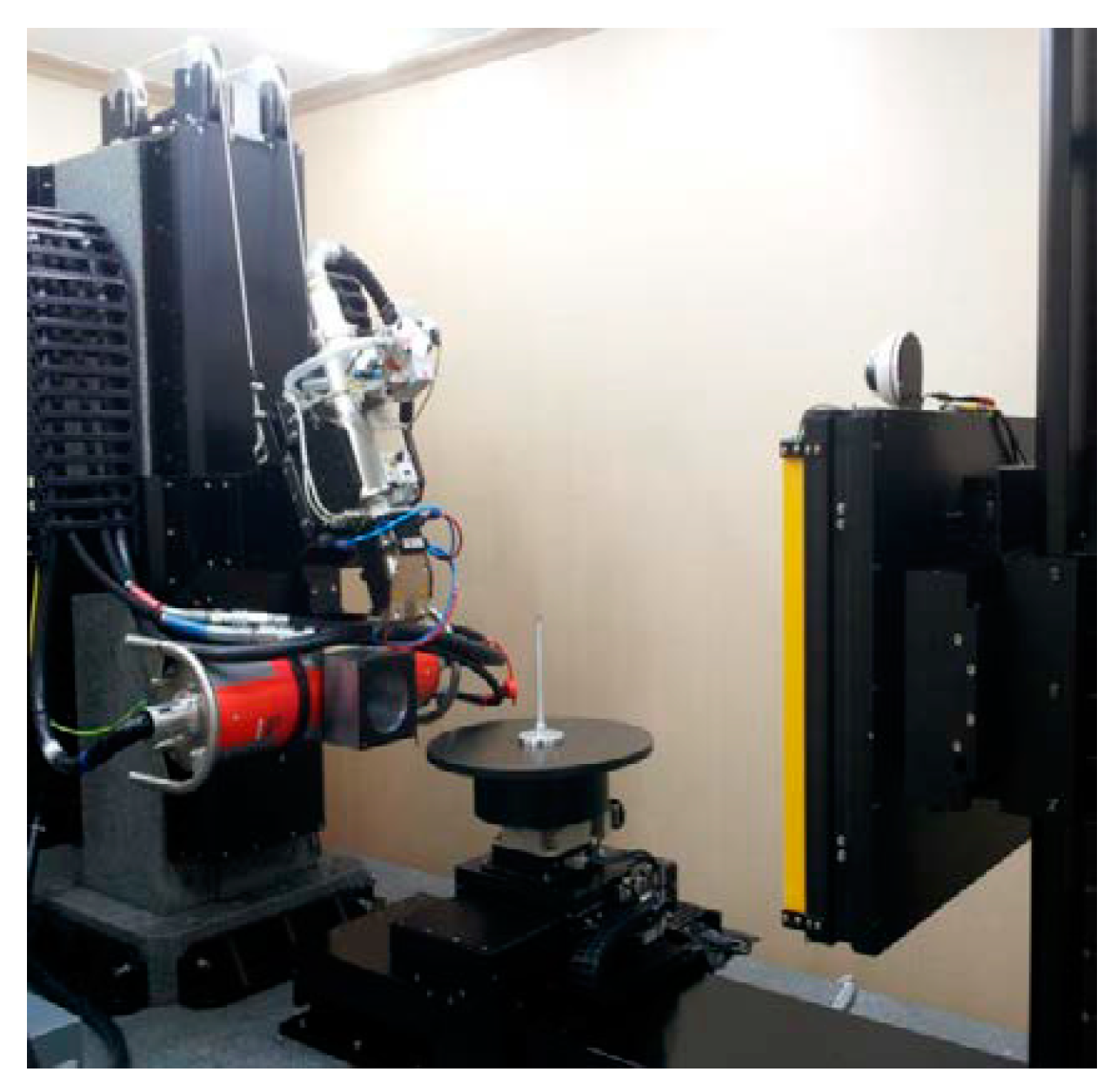
3. Experimental Methods

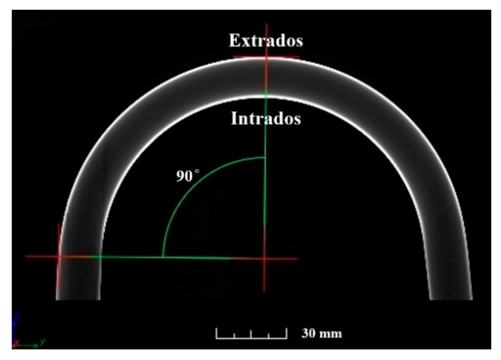
3.1. Computed Tomography (CT) Analysis

Industrial CT is used to create three-dimensional (3D) representations of an object by taking several two-dimensional X-ray images around an axis of rotation and using algorithms to reconstruct a 3D model [17]. CT is used in industry to detect flaws such as voids and cracks, and to perform a particle analysis of a material. CT allows measurements of the external and internal geometry of complex parts. CT is the only method that can measure the inner geometry of a component without the need to cut into and destroy it [18]. CT analysis was performed to more accurately measure the dimensions and shapes of the U-bend tube used in this study. Since the tubes manufactured by the bending process have residual stress, it is difficult to measure the exact dimensions due to deformation of the pipe during cutting. The analysis was performed using high-power CT equipment (TVX-IL450, Techvalley, Korea) as shown in Figure 1, and the 3D digital data were obtained using rotating-transmission scanning with an x-ray and analyzed using VG studio max 3D software [19].

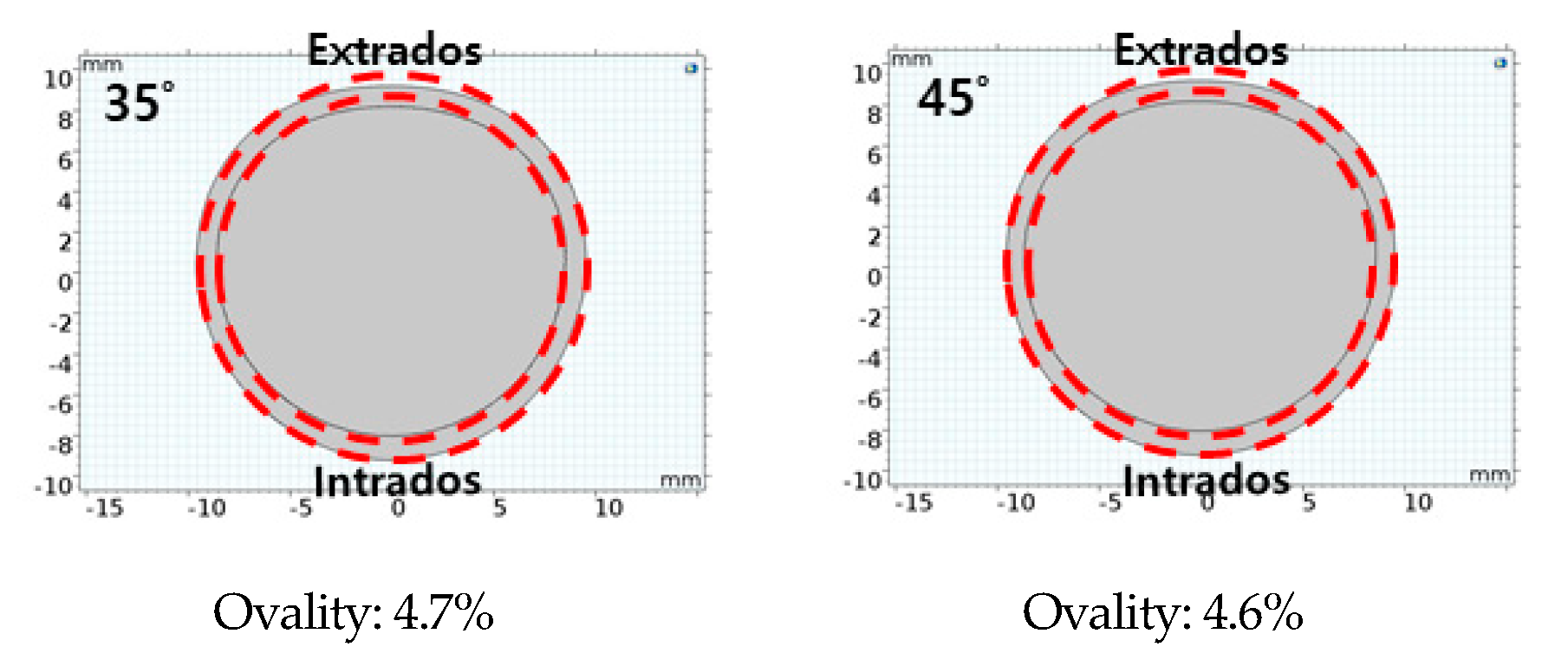
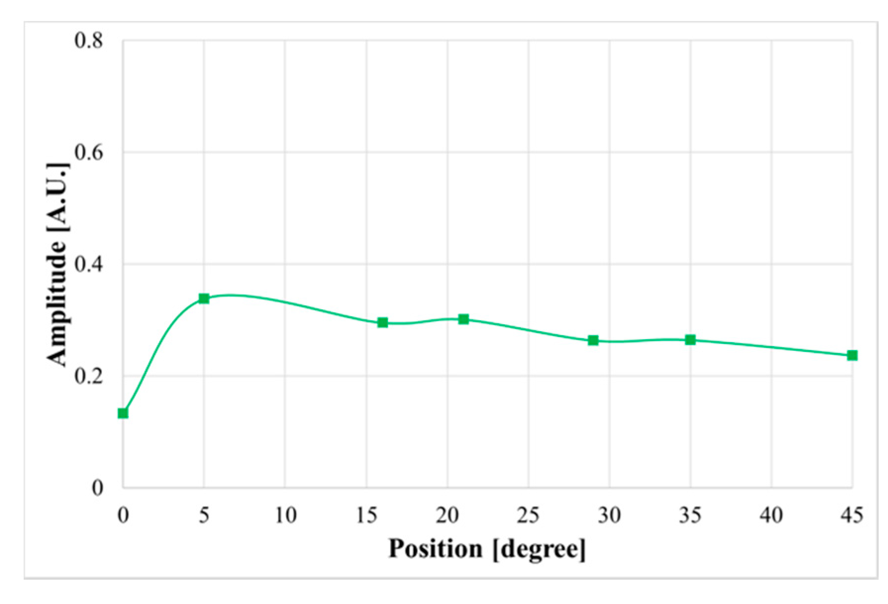
3.2. Tube Curvature Analysis

The three-dimensional images obtained were set up on the decomposition axis to obtain the cross-sectional geometry at the desired angle and location. When the steam generator heat pipe is U-shaped through the bending process, residual stress may exist, or the shape of the cross section may change during the bending process. To confirm the change in shape of the cross section, it can be directly cut and checked, but if the cutting is performed in the presence of residual stress, additional deformation may occur, which makes it difficult to measure the exact dimensions and to apply modeling analysis. The cross-sectional area of a row 1 heat tube was obtained using the cross-sectional axis data of the 3D image (Figure 2). The extrados shown in Figure 2 refer to the outside face of the tube, and the intrados refer to the inside face. The starting point of the left-hand side of the picture was considered to be 0 degrees, and the part corresponding to the outermost angle of the electric tube was considered to be 90 degrees.

Figure 3a shows the cross-sectional shape of the straight tube obtained through CT analysis and axial settings, and Figure 3b shows the cross-sectional shape of the U-bend tube at the 90° position shown in Figure 2. In Figure 3a,b, a yellow dotted line is drawn in a circle to determine the distortion rate. The tubing of the intuition showed that no deformation occurred in the fabrication process, as the shape of the U-shaped tube almost coincides with the yellow dotted line, but the bending process for the U-shaped tube caused tensile stress at the extrados and compression stress at the intrados, resulting in higher ovality. In Figure 3b, the horizontal component is unchanged, but the vertical length is shorter than initial length. During CT measurement, the dimensions were measured based on the internal diameter because the X-ray scattering was pronounced on the outer surface, and the internal diameter of the direct tube averaged 16.94 mm. For U-shaped tubes, the width was 0.15 mm less than the straight line, and the vertical width was 0.66 mm less. The measurement error range was about 0.03 mm, and the ovality was about 4.2% in terms of internal diameter.

$$*Ovality[\%]=\left[\frac{(Max.I.D.-Min.I.D.}{nominal I.D.}\right]\times 100$$

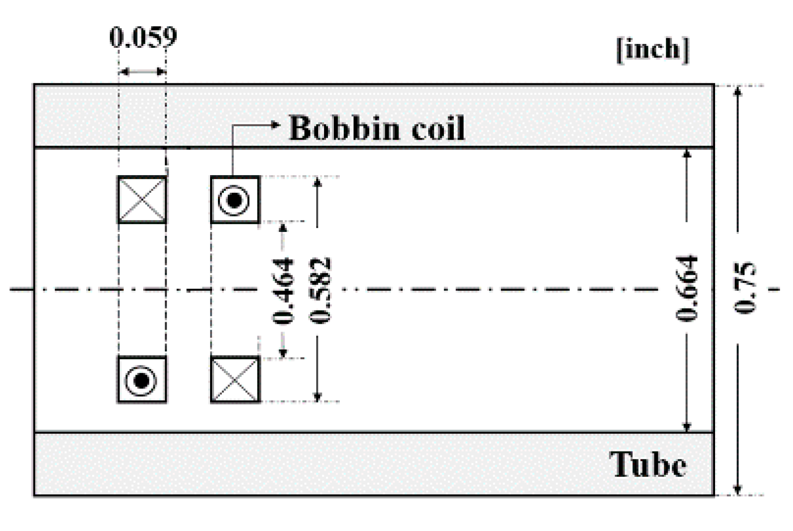
3.3. Geometry Conditions

Figure 4 is a cross-sectional schematic diagram of a bobbin coil, which is a probe used for inspection of the steam generator tube used in the analysis. The bobbin coil was modeled to be placed in the center of the tube by default. The tube material (Inconel 690) and dimensions (19 mm. outer diameter, 0.11 mm. wall thickness) are the same as those used in nuclear power plants in the Republic of Korea. The conductivity of the tube material was $6.76\times {10}^6 \mathrm{S}/\mathrm{m}$, and the relative investment rate of the tube material was 1.01. The size of computational domain, including the air around the specimen, was 3 × 9 in. A boundary condition was imposed so that the tangential component of the magnetic vector potential was zero. The materials of the model were classified into SG tube (Inconel 690), coil (copper), and the remaining part (air).

Table 1. The material properties used in the simulation.

	Relative Permeability	Relative Permittivity	Electrical Conductivity (S/m)
Air	1.00000037	1.000536	3$\times$10−15
Coil (Copper)	0.999994	0.9999996	5.96$\times$107
Tube (Inconel 690)	1.01	1	6.7567$\times$106

shows the properties of each material, including relative permeability, relative permittivity, and electrical conductivity.

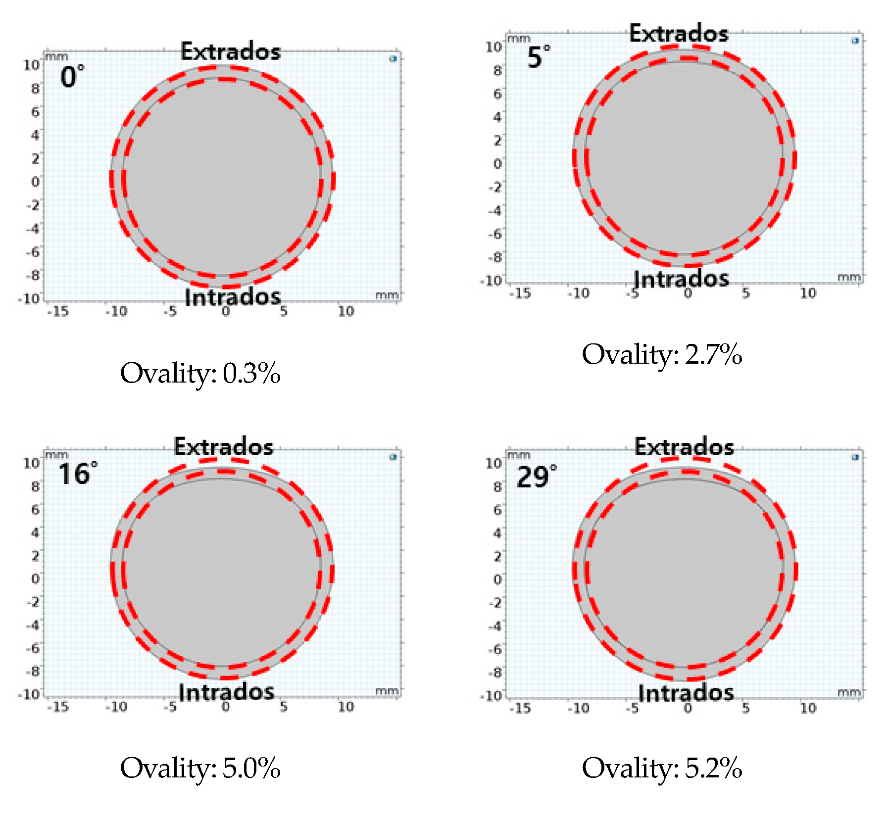
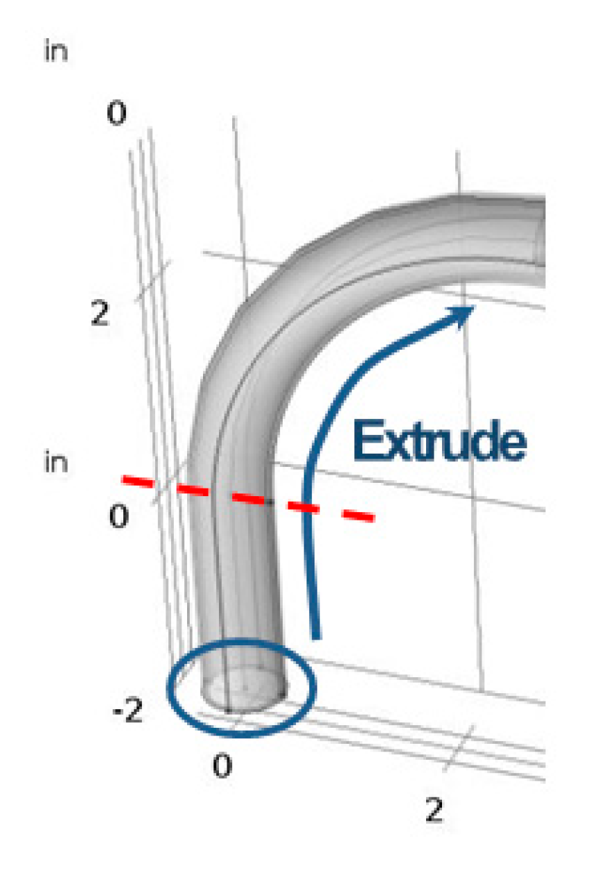
3.4. Curvature Cross-Sectional Area Modeling

The steam generator tube cross-section CT data obtained (Figure 3) are shown in black and white, and can be imported into COMSOL S/W (Figure 5) by calculating the luminance ratio. The sections were obtained by dividing the tubes into six positions (0°, 5°, 16°, 29°, 35°, and 45°), with the outermost part of the tube considered to be 90°, starting at 0° from straight pipe to curved pipe. The red dotted circle in each picture is a circle shape based on 0°. As a result of the elliptical calculation based on the internal diameter described earlier, the elliptical range for each location was 0.3% to 5.2%. Because the shapes of the sections vary depending on the location of the curvature, each section was modeled by extruding three-dimensional pipe curvature (Figure 6) to analyze the effects of the noise signal on the location of the coil.

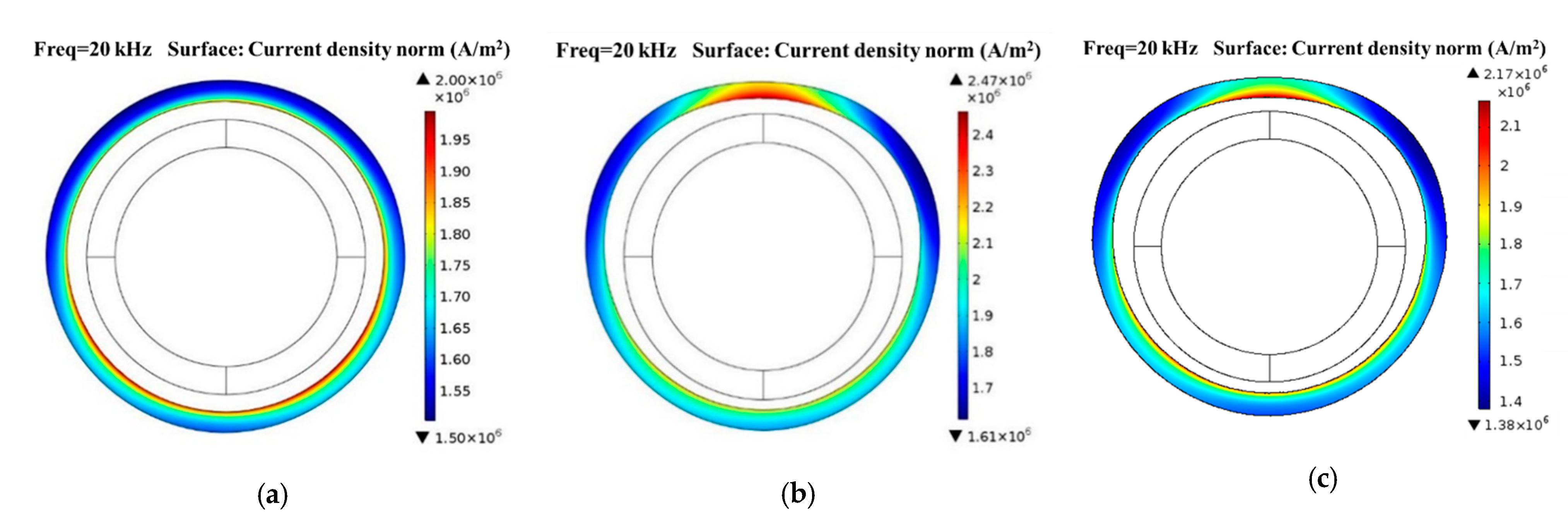
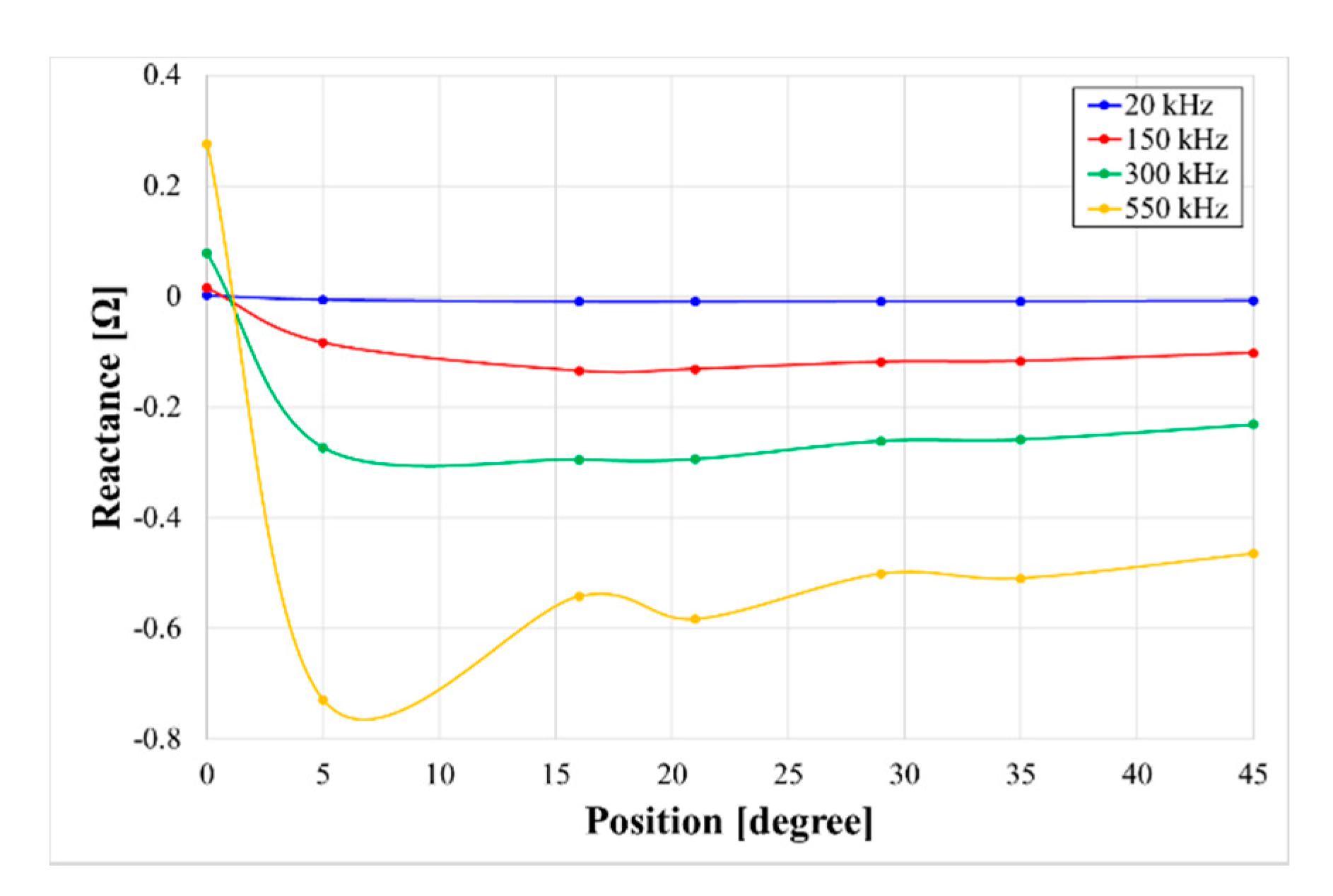
4. Finite Elements Method (FEM) Analysis Results

Based on the conceptual plot in Figure 4, the design conditions were set as boundary conditions for the intervals directly affected by the coil (copper). Frequencies ranging from 20 to 550 kHz are mainly used for inspection of the steam generator at nuclear power plants. To simulate the curved part of the steam generator’s electric tube, six sections were defined according to the location of the curved tube shown in Figure 5 and modeled by extruding a curvature (Figure 6). A total of six types of curved piping were designed, and a coil probe was placed in the angular position to analyze the current density and electric field at each location.

Figure 7 shows the analysis of the distribution of current density in the cross-sectional area at 20 kHz when the coil probe was located at 0°, 29°, and 45° of the U-bend of the electric tube. Since 0° was in the lowest position of ovality and 29° was 5.2%, the highest position of 45° was the outermost angle of the modeled curved pipe. Coil probes were designed to always be located in the middle of the tube, and the frequency 20 kHz was relatively low, so the effects from the pipe’s exterior could be reflected. As shown in Figure 7, increasing the ovality brought the coil probe closer to the inside of the pipe as the pipe deformed. Although the deformation of the piping was mostly concentrated in the extrados region depending on the location, it also partially affected the intrados. The curve begins at 0°, and due to the presence of residual stress during the manufacturing process, we found that the current density increased slightly compared to the extrados due to the slight deformation of the intrados. However, at the 29° and 45° positions of the curve, we found that the current density increased due to the concentration of deformation in the extrados position. Most of the curved sections exhibited a similar overall pattern because of this deformation of the extrados, which can lead to changes in reactance and resistance in the eddy-current test.

Figure 8 shows a three-dimensional analysis of changes in the electric field depending on the coil position at a frequency of 300 kHz. The ovality of the pipe is close to 0.3% at 0°, and the field shown in the coil and pipe is distributed evenly in the direction around the pipe. However, the higher ovality of the pipe resulted in deformation of the inner/external section area, which also partially concentrated the electric field. This is caused by the coil probe entering and leaving the curved section where the electric tube begins to change shape, and by the close distance between the coil and pipe in the inner and outer surface areas. A close area is a sign that that the outer arc surface has contacted the concave section surrounding the coil, and the inner arc surface has contacted the coil in a convex and relatively small area. We predicted that this phenomenon is mainly caused by the curved part of the tube, and would affect the electric field in the coil.

Figure 7 and Figure 8 show that it is difficult to directly compare the amplitude effects on each section because only the current density and electric field effects on the electric tubes generated by the coils are mainly identified. Therefore, it was necessary to analyze the effects of noise at each location to extract the values of the effect and obtain analysis results. Figure 9 shows the reactance change according to the position of the coil in the pipe. The frequency of the general test, between 20 and 300 kHz, showed little change in the value of the reactance due to the difference in ovality, while a difference of about 0.25 was found at a given frequency (550 kHz). This had a strong effect on the curve because the high frequency was relatively concentrated on the near-field effect rather than that the reaction caused noise signal. The change in reaction showed that the value changes early in the interval in which the ovality is transformed, and after a constant deformation, the change had a small effect on the value.

Figure 10 shows the results of the voltage-value analysis based on the reactance and resistance signal values collected during the simulation through condition analysis, for comparison with the impedance values used to determine the signal in the actual test. These values are expressed at a frequency of 300 kHz, indicating that the amplitude change was not significant at all locations, similar to the reactance change. This was estimated to be unaffected by the analytical signal if the current density and electric field are concentrated in a certain part, but the change in overall ovality was small. However, the increase in signal amplitude at the time when the deformation increases from zero requires further analysis.

5. Discussion and Conclusions

In this study, for the ECT inspection of the steam generator tube, we used FEM to detect noise factors generated from curvature to improve fault-detection capabilities. The signal generated by the curvature was found to be one of the sources of noise, and the curvature position may vary in the inner and outer sections due to the bending of the pipe during manufacturing. Using CT analysis, the pipe cross-section was found to have an average oval of about 4.8% compared to the initial curvature. The shape was modeled using a 3D simulation to perform the electromagnetic analysis. The modeling showed that there was a relatively concentrated current density and an electric field in areas with high ovality. However, the ECT signal conversion results showed that the difference in current density does not have a significant effect on the noise signal. Noise signals tend to occur at the starting point of the U-bend in a straight-line tube, and residual stress in the tube is thought to significantly affect the section in which deformation begins. The manufacturing process of the curved tube was found to have a stronger effect on the structure of the inside of the pipe than on changes with a higher sectional ovality of the pipe. The CT analysis suggested that if the coil probe passes through an area where the inside of the coil is not held in a circular shape, a coil may be tilted or shaken. Due to this effect, the noise signal amplitude was greater at the boundary position (between straight and curved tubes) than at the curvature position. Further design-modeling technology development is needed in order to analyze this.

References

1. Rao, B.P.C. Practical Eddy Current testing, Indian Society for Nondestructive Testing–National Certification Board Series; Alpha Sci. Int. Ltd.: Oxford, UK, 2007; pp. 1–25. [Google Scholar]
2. Terry, H.; Mike, W. Eddy Current Testing Technology; Eclipse Scientific Products Inc.: Oshawa, ON, Canada, 2012; pp. 1–6. [Google Scholar]
3. Einav, I. Non-destructive Testing for Plant Life Assessment; International Atomic Energy Agency: Vienna, Austria, 2005; pp. 1–61. [Google Scholar]
4. Zhang, Y.H.; Luo, F.L.; Sun, H.X. Impedance Evaluation of a Probe-Coil’s Lift-off and Tilt Effect in Eddy-Current Nondestructive Inspection by 3D Finite Element Modeling. In Proceedings of the 17th World Conference on Nondestructive Testing, Shanghai, China, 25–28 October 2008. [Google Scholar]
5. Bakhtiari, S.; Kupperman, D.S. Modeling of eddy current probe response for steam generator tubes. Nucl. Eng. Des. 1999, 194, 57–71. [Google Scholar] [CrossRef] [Green Version]
6. Johnston, D.P.; Buck, J.A.; Underhill, P.R.; Morelli, J.E.; Krause, T.W. Pulsed eddy-current detection of loose parts in steam generators. IEEE Sens. J. 2018, 18, 2506–2512. [Google Scholar] [CrossRef]
7. Jung, H.S.; Kweon, Y.H.; Lee, D.H.; Shin, W.J.; Yim, C.K. Detection of Foreign Objects using Bobbin Probe in Eddy Current Test. J. Korean Soc. Nondestruct. Test. 2016, 36, 295–299. [Google Scholar] [CrossRef] [Green Version]
8. Buck, J.A.; Underhill, P.R.; Morelli, J.; Krause, T.W. Simultaneous multi-parameter measurement in pulsed eddy current steam generator data using artificial neural networks. IEEE Trans. Instrum. Meas. 2016, 65, 672–679. [Google Scholar] [CrossRef]
9. Sophian, A.; Tian, G.Y.; Taylor, D.; Rudlin, J. A feature extraction technique based on principal component analysis for pulsed eddy current NDT. NDT E Int. 2003, 36, 37–41. [Google Scholar] [CrossRef]
10. Xin, J.J. Design and Analysis of Rotating Field Eddy Current Probe for Tube Inspection. Ph. D. Thesis, Department of Electronic Engineering, Michigan State University, East Lansing, MI, USA, 2014; pp. 46–63. [Google Scholar]
11. Sadiku, M.N.O. Elements of Electromagnetics; Oxford Univ. Press, Inc.: New York, NY, USA, 2001; pp. 261–392. [Google Scholar]
12. Palanisamy, R. Finite Element Modeling of Eddy Current Nondestructive Testing Phenomena. Ph. D. Thesis, Department of Electronic Engineering, Colorado State University, Fort Collins, CO, USA, 1980; pp. 23–90. [Google Scholar]
13. Ida, N.; Betzold, K.; Lord, W. Finite Element Modeling of Absolute Eddy Current Probe Signals. J. Nondestr. Eval. 1982, 3, 147–154. [Google Scholar] [CrossRef]
14. Bennoud, S.; Zergoug, M. Modeling and Simulation for 3D Eddy Current Testing in Conduction Materials. Int. J. Mech. Aerosp. Ind. Mechatron. Eng. 2014, 8, 754–757. [Google Scholar]
15. Song, S.J.; Shin, Y.K. Eddy Current Flaw Characterization in Tubes by Neural Networks and Finite Element Modeling. J. NDT E Int. 2000, 33, 233–243. [Google Scholar] [CrossRef]
16. Shin, Y.K.; Song, S.C.; Jung, H.S.; Lee, Y.T. Prediction and Analysis of ECT Signals due to Tube Defects near Support Plate in Steam Generator. J. Key Eng. Mater. 2006, 321–323, 420–425. [Google Scholar] [CrossRef]
17. Rosell, A. Finite Element Modelling of Eddy Current Nondestructive Evaluation in Probability of Detection Studies; Department Applied Mechanics, Chalmers University: Göteborg, Sweden, 2012; pp. 13–28. [Google Scholar]
18. Thompson, A.; Maskery, I.; Leach, R.K. X-ray Computed Tomography for Additive Manufacturing: A review. Meas. Sci. Technol. 2016, 27, 072001. [Google Scholar] [CrossRef]
19. De Chiffre, L.; Carmignato, S.; Kruth, J.-P.; Schmitt, R.; Weckenmann, A. Industrial Applications of Computed Tomography. CIRP Ann. Manuf. Technol. 2014, 63, 655–677. [Google Scholar] [CrossRef]
Figure 1. The CT(Computed Tomography) equipment with a high-power X-ray tube (450 kV/max, 1500 W).
Applsci 11 00696 g001
Figure 2. The results of the CT analysis of the U-bend tube.
Applsci 11 00696 g002
Figure 3. The cross-sectional areas from the CT analysis for the: (a) straight tube and (b) U-bend tube.
Applsci 11 00696 g003
Figure 4. The schematic diagram of the simulation analysis model.
Applsci 11 00696 g004
Figure 5. The analysis results for the 2D modeling using the simulation software.
Applsci 11 00696 g005aApplsci 11 00696 g005b
Figure 6. A simulation modeling concept of a U-bend tube.
Applsci 11 00696 g006
Figure 7. The results of the simulations of current density at angle positions: (a) 0°, (b) 29°, and (c) 45°.
Applsci 11 00696 g007
Figure 8. The results of the simulation of the electric field at angle positions: (a) 0°, (b) 29°, and (c) 45°.
Applsci 11 00696 g008
Figure 9. Comparison of reactance by coil position and CSA (Cross Sectional Area) variation.
Applsci 11 00696 g009
Figure 10. The amplitude variation with coil position of the simulation analysis results.
Applsci 11 00696 g010