Hybrid Encoding Scheme for AMBTC Compressed Images Using Ternary Representation Technique


Abstract
1. Introduction
2. Related Works
2.1. The AMBTC Method
2.2. Xiang et al.’s Method
- (1)
- If only rules 1 or 2 are met, group or needs to be subdivided. The number of pixels needing to be subdivided is denoted by , and bitmap or has to be used to record the bitmap of or . In this case, block is eventually divided into three groups.
- (2)
- If both rules 1 and 2 are met, both and need to be subdivided, and block is eventually divided into four groups. Bitmap and have to be recorded to maintain the grouping information.
3. Proposed Method
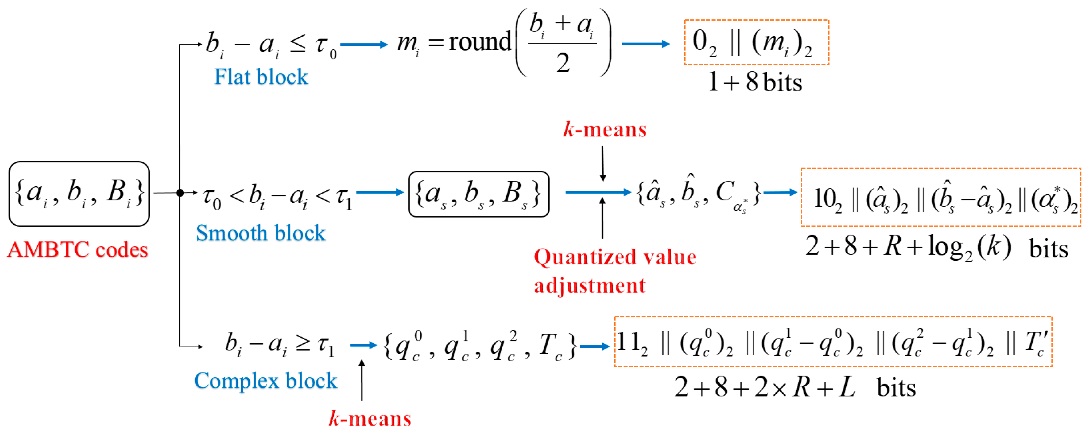
3.1. Encoding of Flat Blocks
3.2. Encoding of Smooth Blocks
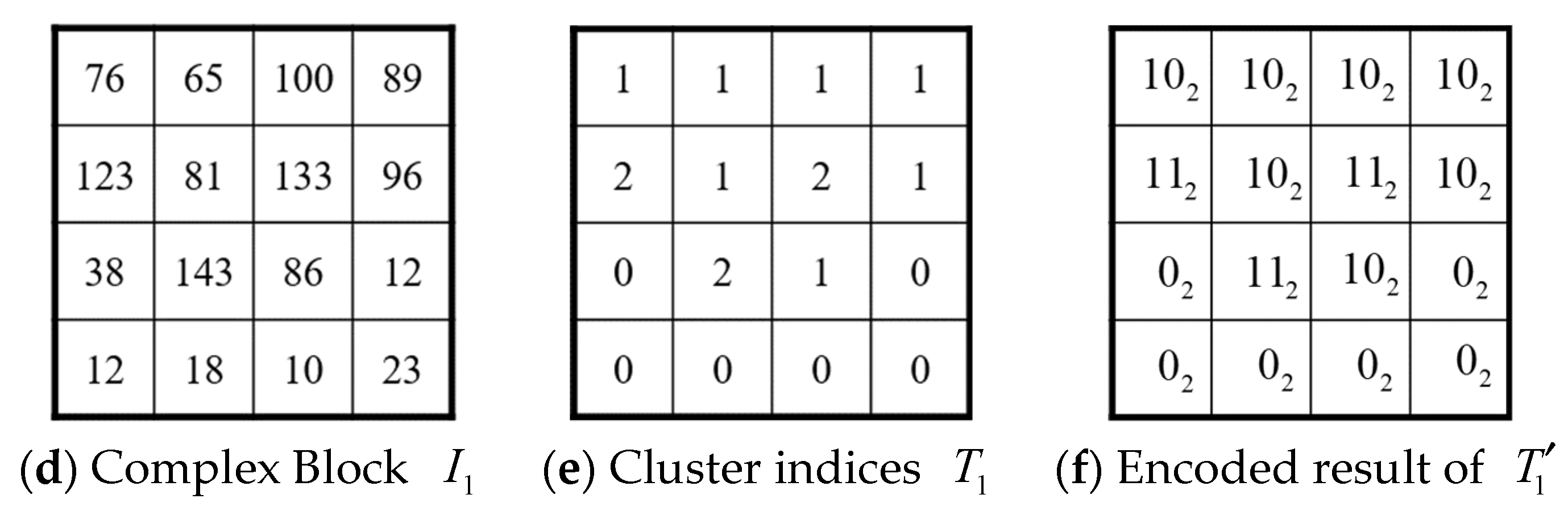
3.3. Encoding of Complex Blocks
3.4. Encoding Procedures
- Input:
- Original image , block size , thresholds and , parameter , and cluster size .
- Output:
- Code stream .
- Step 1:
- Partition the original image into blocks of size . Encode using the AMBTC encoder and obtain codes , as described in Section 2.1.
- Step 2:
- Scan codes . Let be the bitmap of smooth blocks. Clustering into groups using the k-means clustering algorithm, we obtain cluster centers and cluster indices . Concatenate the binary representation of and obtain the concatenated code stream . The pairs of adjusted quantized values of smooth blocks are also obtained, as described in Section 3.2. Similarly, quantized values and ternary maps of complex blocks are also obtained, as described in Section 3.3.
- Step 3:
- Scan codes again and perform the encoding according to the cases listed below:
- Case 1:
- If , a flat block is visited and the code stream of block is .
- Case 2:
- If , a smooth block is visited. Extract , , and from obtained in Step 2, and block is encoded by . Note that is encoded using the DES, as described in Section 2.2.
- Case 3:
- If , block is a complex one. Extract , , , and from obtained in Step 2, and block is encoded by . Note that and are encoded using the DES (see Section 2.2).
- Step 4:
- Repeat Step 3 until the code stream of blocks are obtained. Concatenate , we have the concatenated code stream .
- Step 5:
- Concatenate and ; we obtain the final code stream of image , i.e., .
3.5. Decoding Procedures
- Input:
- Code stream , block size , parameter , , and cluster size .
- Output:
- Decompressed image .
- Step 1:
- Extract from and reconstruct cluster centers .
- Step 2:
- Extract one bit from . According to the extracted bit, one of the following decoding cases is then performed:
- Case 1:
- If , the block to be reconstructed is a flat block. All the pixel values of block are the decimal value of the next 8 bits extracted from .
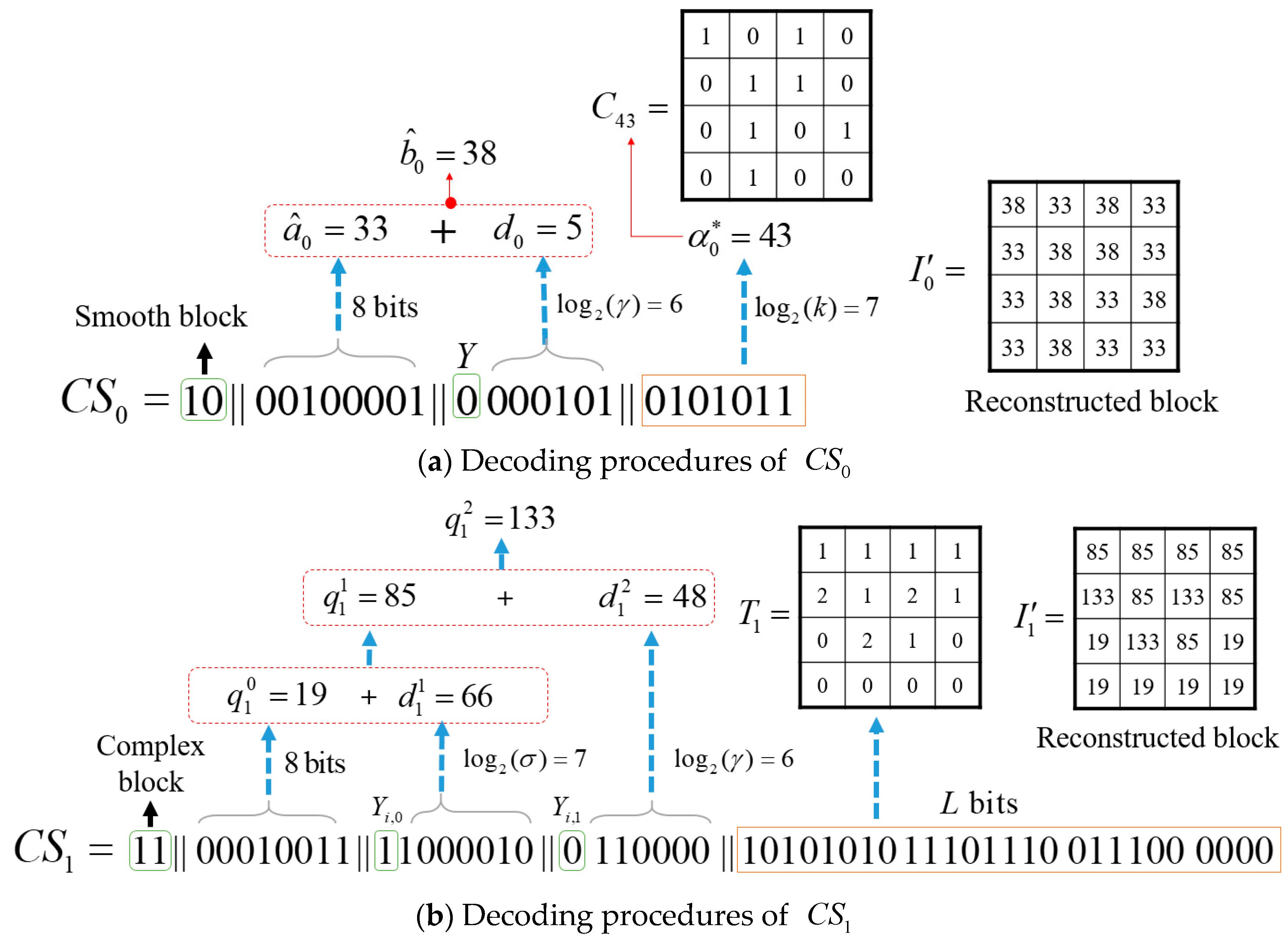
- Case 2:
- If and the next extracted bit is , the block to be reconstructed is a smooth block. Extract the next 8 bits and convert them to a decimal value to obtain the quantized value . Read the next bit from . If the read bit is , is reconstructed by the decimal value of the next bits plus . Otherwise, is reconstructed by the decimal value of next bits plus . The clustering index is the decimal value of next bits, and the bitmap can be obtained from . Using the AMBTC decoder to decode , the image block can be reconstructed.
- Case 3:
- If and the next extracted bits is , the block to be reconstructed is a complex block. Extract the next 8 bits and convert them to a decimal value to obtain the quantized value . Read the next bit from . If the read bit is , is reconstructed by the plus the decimal value of the next bits; otherwise, is reconstructed by the decimal value of the next bits plus . Using a similar manner, is reconstructed. To reconstruct the ternary map , we start from to and repeat the following process: Read a bit from . If , we have . Otherwise, read the next bit from . If , . If , . Once we have and , the j-th pixel of the image block is reconstructed by , , or if , 1, or 2, respectively.
- Step 3:
- Repeat Step 2 until all image blocks are reconstructed, and the final decompressed image is obtained.
4. Experimental Results
4.1. The Performance of the Proposed Method
4.1.1. Coding Efficiency Comparisons
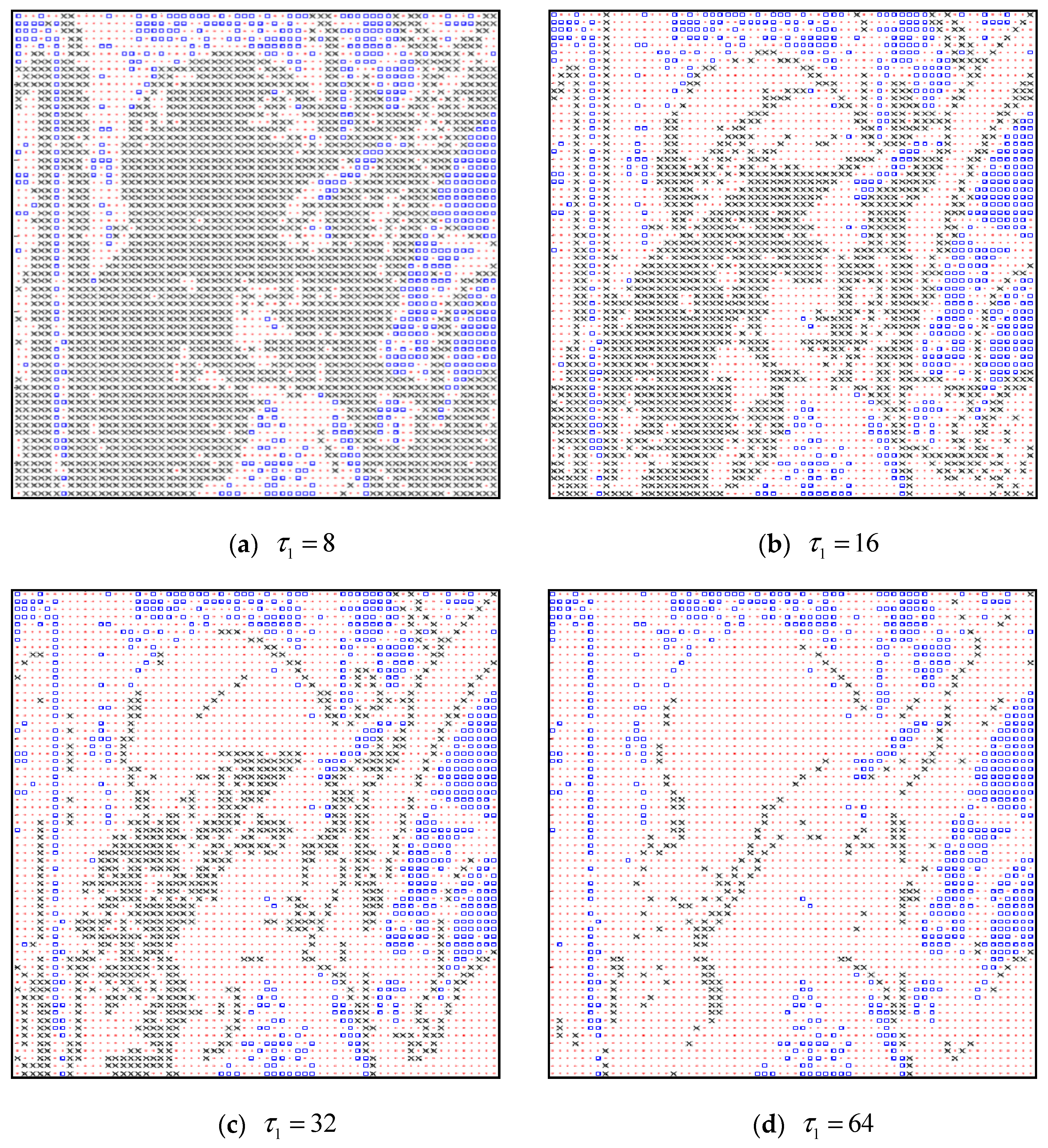
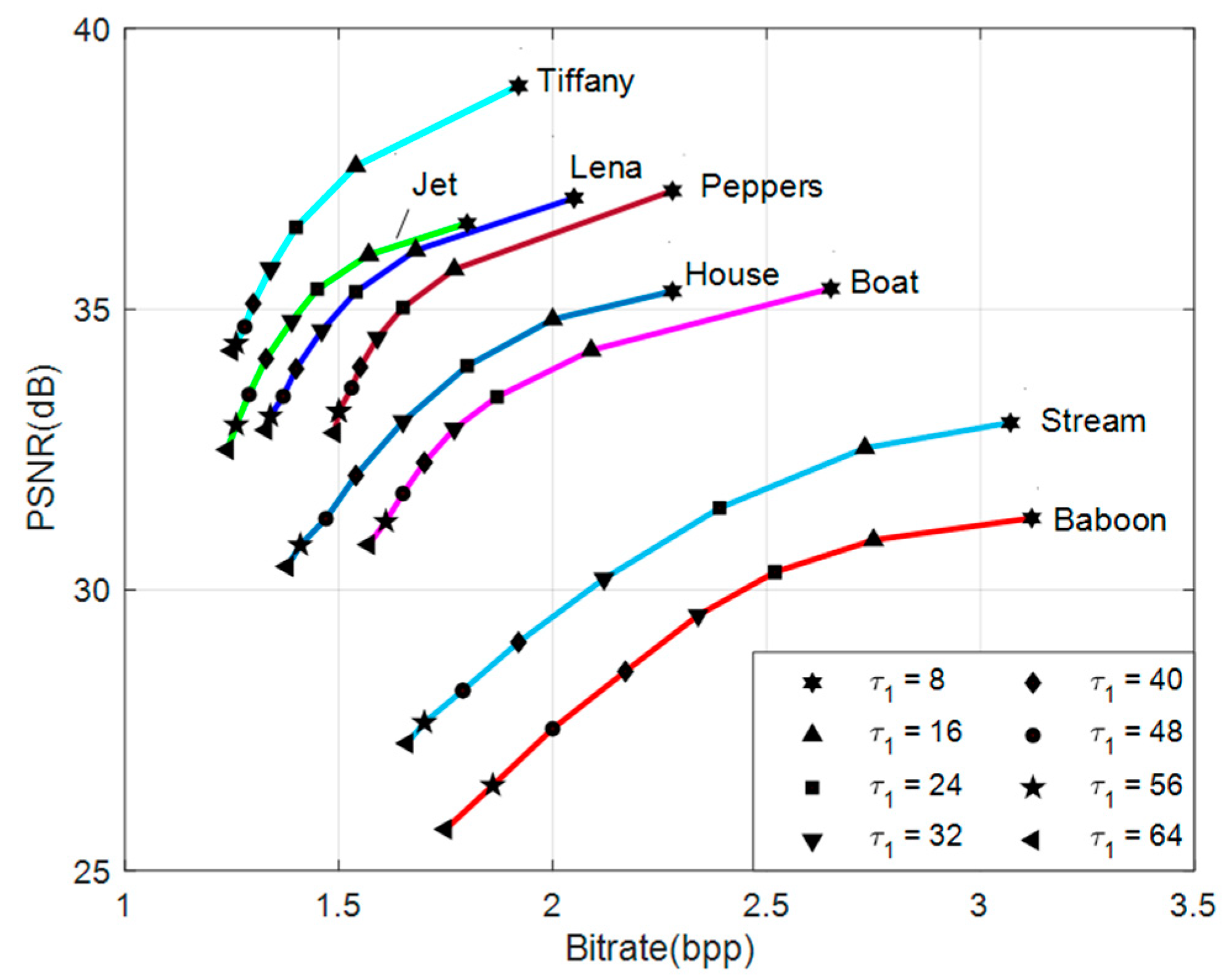
4.1.2. Performance Comparison of Various
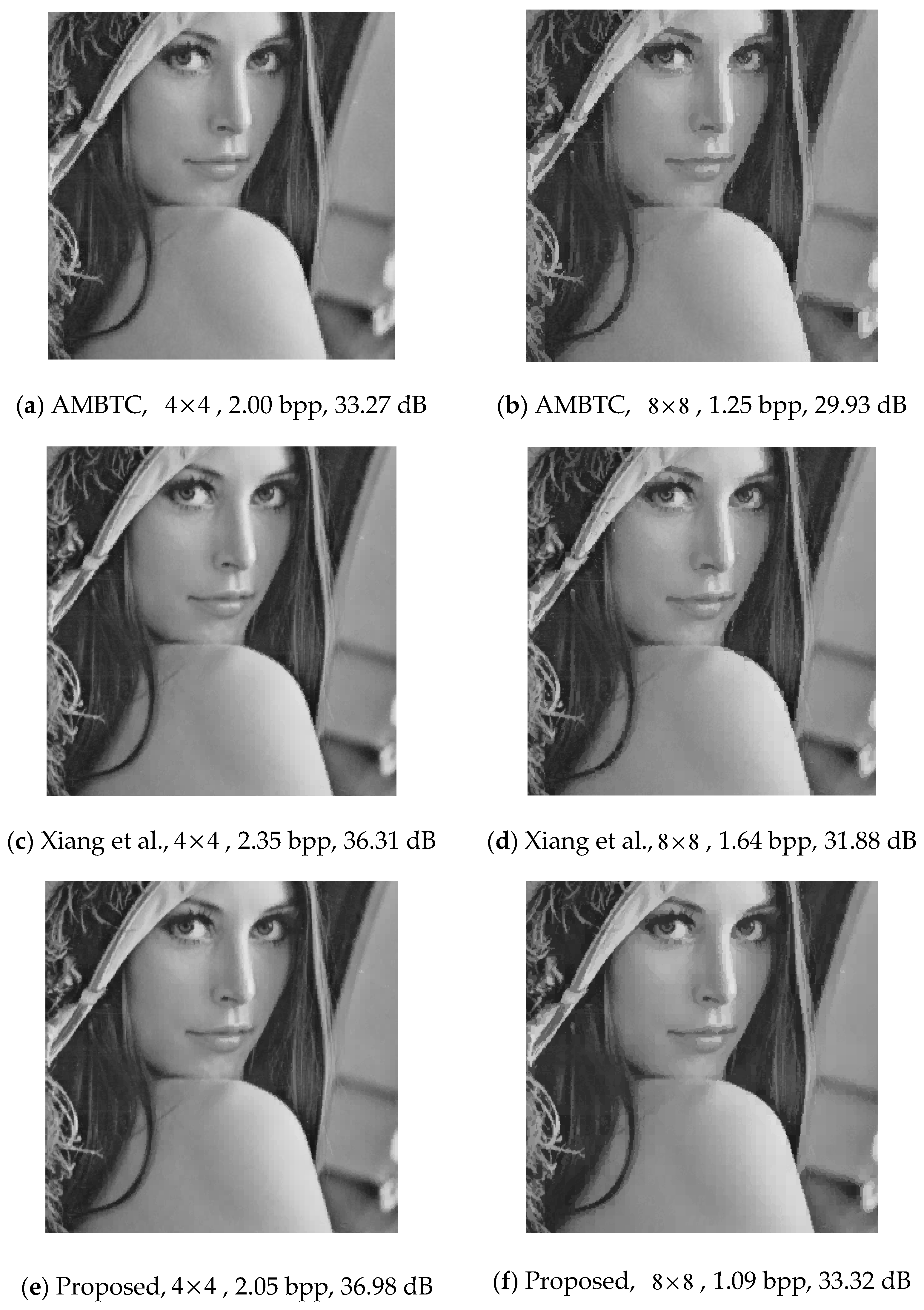
4.2. Comparisons with Xiang et al.’s Work
5. Conclusions
Author Contributions
Funding
Institutional Review Board Statement
Informed Consent Statement
Data Availability Statement
Conflicts of Interest
References
- Liu, J.; Tian, Y.-G.; Han, T.; Yang, C.-F.; Liu, W.-B. LSB steganographic payload location for JPEG-decompressed images. Digit. Signal Process. 2015, 38, 66–76. [Google Scholar] [CrossRef]
- Liu, J.; Tian, Y.; Han, T.; Wang, J.; Luo, X. Stego key searching for LSB steganography on JPEG decompressed image. Sci. China Inf. Sci. 2016, 59, 1–15. [Google Scholar] [CrossRef]
- Qin, C.; Chang, C.-C.; Chiu, Y.-P. A Novel Joint Data-Hiding and Compression Scheme Based on SMVQ and Image Inpainting. IEEE Trans. Image Process. 2014, 23, 969–978. [Google Scholar] [CrossRef]
- Qin, C.; Hu, Y.-C. Reversible data hiding in VQ index table with lossless coding and adaptive switching mechanism. Signal Process. 2016, 129, 48–55. [Google Scholar] [CrossRef]
- Tsou, C.-C.; Hu, Y.-C.; Chang, C.-C. Efficient optimal pixel grouping schemes for AMBTC. Imaging Sci. J. 2008, 56, 217–231. [Google Scholar] [CrossRef]
- Hu, Y.C.; Su, B.H.; Tsai, P.Y. Color image coding scheme using absolute moment block and prediction technique. Imaging Sci. J. 2008, 56, 254–270. [Google Scholar] [CrossRef]
- Delp, E.J.; Mitchell, O.R. Image coding using block truncation coding. IEEE Trans. Commun. 1979, 27, 1335–1342. [Google Scholar] [CrossRef]
- Lema, M.; Mitchell, O. Absolute Moment Block Truncation Coding and Its Application to Color Images. IEEE Trans. Commun. 1984, 32, 1148–1157. [Google Scholar] [CrossRef]
- Kumaravadivelan, A.; Nagaraja, P.; Sudhanesh, R. Video compression technique through block truncation coding. Int. J. Res. Anal. Rev. 2019, 6, 236–242. [Google Scholar]
- Hemida, O.; He, H. A self-recovery watermarking scheme based on block truncation coding and quantum chaos map. Multimed. Tools Appl. 2020, 79, 18695–18725. [Google Scholar] [CrossRef]
- Qin, C.; Ji, P.; Zhang, X.; Dong, J.; Wang, J. Fragile image watermarking with pixel-wise recovery based on overlapping embedding strategy. Signal Process. 2017, 138, 280–293. [Google Scholar] [CrossRef]
- Qin, C.; Ji, P.; Chang, C.-C.; Dong, J.; Sun, X. Non-uniform Watermark Sharing Based on Optimal Iterative BTC for Image Tampering Recovery. IEEE MultiMed. 2018, 25, 36–48. [Google Scholar] [CrossRef]
- Ma, Y.Y.; Luo, X.Y.; Li, X.L.; Bao, Z.; Zhang, Y. Selection of rich model steganalysis features based on decision rough set α-positive region reduction. IEEE Trans. Circuits Syst. Video Technol. 2019, 29, 336–350. [Google Scholar] [CrossRef]
- Zhang, Y.; Qin, C.; Zhang, W.M.; Liu, F.L.; Luo, X.Y. On the fault-tolerant performance for a class of robust image ste-ganography. Signal Process. 2018, 146, 99–111. [Google Scholar] [CrossRef]
- Hu, Y.-C. Low-complexity and low-bit-rate image compression scheme based on absolute moment block truncation coding. Opt. Eng. 2003, 42, 1964–1975. [Google Scholar] [CrossRef]
- Xiang, Z.; Hu, Y.-C.; Yao, H.; Qin, C. Adaptive and dynamic multi-grouping scheme for absolute moment block truncation coding. Multimed. Tools Appl. 2018, 78, 7895–7909. [Google Scholar] [CrossRef]
- Chen, W.-L.; Hu, Y.-C.; Liu, K.-Y.; Lo, C.-C.; Wen, C.-H. Variable-Rate Quadtree-segmented Block Truncation Coding for Color Image Compression. Int. J. Signal Process. Image Process. Pattern Recognit. 2014, 7, 65–76. [Google Scholar] [CrossRef]
- Hong, W. Efficient Data Hiding Based on Block Truncation Coding Using Pixel Pair Matching Technique. Symmetry 2018, 10, 36. [Google Scholar] [CrossRef]
- Mathews, J.; Nair, M.S. Adaptive block truncation coding technique using edge-based quantization approach. Comput. Electr. Eng. 2015, 43, 169–179. [Google Scholar] [CrossRef]
- Hartigan, J.A.; Wong, M.A. A K-means clustering algorithm. Appl. Stat. 1979, 28, 100–108. [Google Scholar] [CrossRef]
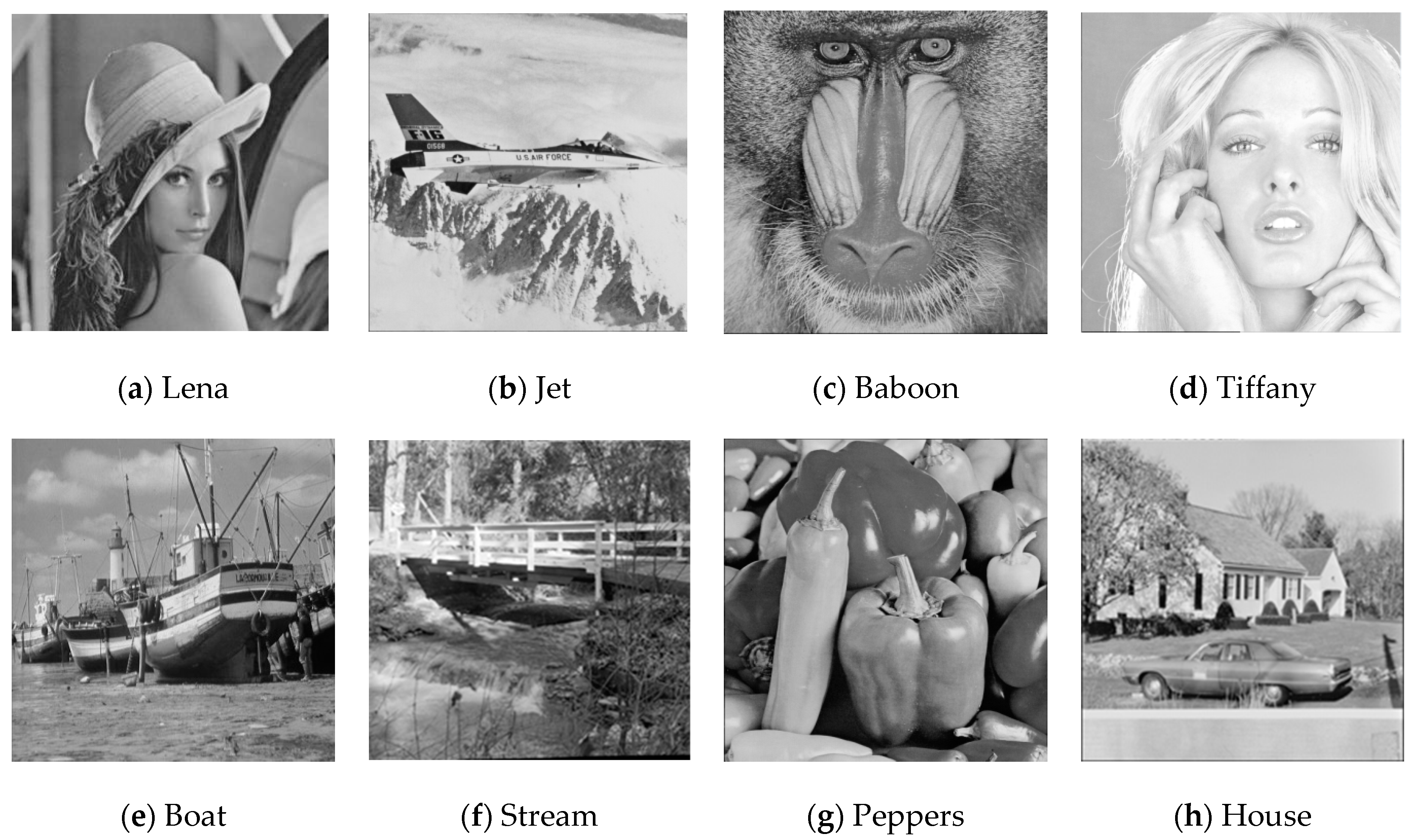
- The USC-SIPI Image Database. Available online: http://sipi.usc.edu/database/ (accessed on 1 November 2020).


| Number of Groups | Number of Bits | |
|---|---|---|
| 1 | ||
| 2 | ||
| 3 | or | |
| 4 |
| Images | |||||||||
|---|---|---|---|---|---|---|---|---|---|
| Bitrate | w/o QA | w/QA | Bitrate | w/o QA | w/QA | Bitrate | w/o QA | w/QA | |
| Lena | 1.60 | 35.83 | 35.96 | 1.63 | 35.95 | 36.05 | 1.68 | 36.07 | 36.15 |
| Jet | 1.52 | 35.85 | 35.91 | 1.55 | 35.92 | 35.97 | 1.58 | 35.99 | 36.03 |
| Baboon | 2.73 | 30.80 | 30.85 | 2.76 | 30.85 | 30.89 | 2.79 | 30.89 | 30.93 |
| Tiffany | 1.47 | 37.18 | 37.38 | 1.50 | 37.39 | 37.55 | 1.55 | 37.57 | 37.69 |
| Boat | 2.00 | 33.97 | 34.13 | 2.05 | 34.15 | 34.27 | 2.10 | 34.27 | 34.36 |
| Stream | 2.68 | 32.43 | 32.49 | 2.70 | 32.49 | 32.53 | 2.73 | 32.55 | 32.57 |
| Peppers | 1.68 | 35.34 | 35.57 | 1.73 | 35.52 | 35.71 | 1.78 | 35.71 | 35.85 |
| House | 1.95 | 34.73 | 34.78 | 1.97 | 34.79 | 34.82 | 2.01 | 34.85 | 34.88 |
| Average | 1.95 | 34.52 | 34.63 | 1.99 | 34.63 | 34.72 | 2.03 | 34.74 | 34.81 |
| Images | |||||||||
|---|---|---|---|---|---|---|---|---|---|
| Bitrate | w/o QA | w/QA | Bitrate | w/o QA | w/QA | Bitrate | w/o QA | w/QA | |
| Lena | 0.97 | 32.96 | 33.07 | 1.01 | 33.03 | 33.12 | 1.08 | 33.13 | 33.21 |
| Jet | 1.00 | 32.77 | 32.82 | 1.04 | 32.83 | 32.86 | 1.11 | 32.90 | 32.92 |
| Baboon | 1.79 | 28.67 | 28.72 | 1.83 | 28.72 | 28.75 | 1.89 | 28.80 | 28.82 |
| Tiffany | 0.89 | 34.63 | 34.81 | 0.93 | 34.79 | 34.93 | 1.00 | 34.99 | 35.09 |
| Boat | 1.30 | 31.17 | 31.32 | 1.34 | 31.24 | 31.37 | 1.41 | 31.36 | 31.46 |
| Stream | 1.89 | 29.79 | 29.82 | 1.92 | 29.84 | 29.86 | 1.99 | 29.93 | 29.93 |
| Peppers | 1.01 | 32.59 | 32.74 | 1.05 | 32.66 | 32.80 | 1.12 | 32.79 | 32.90 |
| House | 1.36 | 31.52 | 31.57 | 1.39 | 31.57 | 31.61 | 1.46 | 31.65 | 31.67 |
| Average | 1.28 | 31.76 | 31.86 | 1.31 | 31.83 | 31.91 | 1.38 | 31.94 | 32.00 |
| Images | AMBTC bpp = 2.0 | PSNR (dB) | Bitrate (bpp) | ||||
|---|---|---|---|---|---|---|---|
| Lena | 33.24 | 36.05 | 34.62 | 32.85 | 1.68 | 1.46 | 1.33 |
| Jet | 31.97 | 35.98 | 34.79 | 32.50 | 1.56 | 1.39 | 1.24 |
| Baboon | 26.98 | 30.89 | 29.55 | 25.74 | 2.75 | 2.34 | 1.75 |
| Tiffany | 35.77 | 37.55 | 35.72 | 34.26 | 1.54 | 1.34 | 1.25 |
| Boat | 31.16 | 34.27 | 32.87 | 30.81 | 2.09 | 1.77 | 1.57 |
| Stream | 28.59 | 32.53 | 30.20 | 27.27 | 2.73 | 2.11 | 1.66 |
| Peppers | 33.42 | 35.71 | 34.49 | 32.80 | 1.77 | 1.59 | 1.49 |
| House | 30.89 | 34.82 | 32.00 | 30.42 | 2.00 | 1.65 | 1.38 |
| Average | 31.50 | 34.73 | 33.03 | 30.83 | 2.02 | 1.71 | 1.46 |
| Images | AMBTC bpp = 1.25 | PSNR (dB) | Bitrate (bpp) | ||||
|---|---|---|---|---|---|---|---|
| Lena | 29.93 | 33.12 | 31.80 | 29.24 | 1.02 | 0.76 | 0.51 |
| Jet | 28.84 | 32.86 | 31.72 | 29.40 | 1.04 | 0.82 | 0.62 |
| Baboon | 25.18 | 28.75 | 27.66 | 23.06 | 1.81 | 1.43 | 0.71 |
| Tiffany | 32.55 | 34.93 | 32.76 | 30.74 | 0.94 | 0.62 | 0.47 |
| Boat | 28.07 | 31.37 | 29.78 | 27.44 | 1.35 | 0.90 | 0.61 |
| Stream | 26.10 | 29.85 | 27.99 | 24.18 | 1.92 | 1.34 | 0.63 |
| Peppers | 29.66 | 32.80 | 31.49 | 29.43 | 1.06 | 0.78 | 0.58 |
| House | 27.68 | 31.60 | 30.20 | 26.92 | 1.39 | 1.02 | 0.62 |
| Average | 28.50 | 31.91 | 30.43 | 27.55 | 1.32 | 0.96 | 0.59 |
| Images | Metrics | Proposed | [16] | Proposed | [16] | Proposed | [16] |
|---|---|---|---|---|---|---|---|
| Lena | PSNR | 36.98 | 36.31 | 36.05 | 35.12 | 35.31 | 33.91 |
| Bitrate | 2.05 | 2.35 | 1.68 | 2.20 | 1.54 | 1.95 | |
| Jet | PSNR | 36.53 | 34.96 | 35.97 | 33.74 | 35.36 | 32.69 |
| Bitrate | 1.80 | 1.98 | 1.57 | 1.87 | 1.45 | 1.71 | |
| Baboon | PSNR | 31.28 | 31.40 | 30.89 | 29.59 | 30.32 | 28.11 |
| Bitrate | 3.12 | 3.57 | 2.75 | 3.24 | 2.52 | 2.75 | |
| Tiffany | PSNR | 38.98 | 38.42 | 37.55 | 37.29 | 36.46 | 36.41 |
| Bitrate | 1.92 | 2.12 | 1.54 | 1.99 | 1.40 | 1.81 | |
| Boat | PSNR | 35.37 | 34.81 | 34.27 | 33.43 | 33.44 | 32.11 |
| Bitrate | 2.65 | 3.02 | 2.09 | 2.79 | 1.87 | 2.43 | |
| Stream | PSNR | 32.98 | 32.69 | 32.53 | 31.14 | 31.46 | 29.69 |
| Bitrate | 3.07 | 3.45 | 2.73 | 3.18 | 2.39 | 2.75 | |
| Peppers | PSNR | 37.11 | 36.38 | 35.71 | 35.23 | 35.03 | 34.16 |
| Bitrate | 2.28 | 2.64 | 1.77 | 2.45 | 1.65 | 2.20 | |
| House | PSNR | 35.32 | 35.06 | 34.82 | 33.52 | 33.99 | 31.86 |
| Bitrate | 2.28 | 2.52 | 2.00 | 2.35 | 1.80 | 2.05 |
| Images | Metrics | Proposed | [16] | Proposed | [16] | Proposed | [16] |
|---|---|---|---|---|---|---|---|
| Lena | PSNR | 33.32 | 31.88 | 32.66 | 30.85 | 32.00 | 30.27 |
| Bitrate | 1.09 | 1.64 | 0.90 | 1.45 | 0.79 | 1.27 | |
| Jet | PSNR | 32.99 | 30.37 | 32.44 | 29.66 | 31.87 | 29.23 |
| Bitrate | 1.09 | 1.36 | 0.94 | 1.24 | 0.84 | 1.13 | |
| Baboon | PSNR | 28.84 | 28.14 | 28.43 | 26.44 | 27.84 | 25.50 |
| Bitrate | 1.88 | 2.23 | 1.65 | 1.88 | 1.47 | 1.50 | |
| Tiffany | PSNR | 35.36 | 34.44 | 33.97 | 33.48 | 32.95 | 32.89 |
| Bitrate | 1.04 | 1.51 | 0.77 | 1.33 | 0.64 | 1.16 | |
| Boat | PSNR | 31.62 | 30.12 | 30.68 | 29.11 | 29.95 | 28.54 |
| Bitrate | 1.46 | 1.99 | 1.11 | 1.75 | 0.93 | 1.50 | |
| Stream | PSNR | 29.94 | 28.62 | 29.39 | 27.30 | 28.31 | 26.54 |
| Bitrate | 1.99 | 2.20 | 1.71 | 1.90 | 1.41 | 1.58 | |
| Peppers | PSNR | 33.01 | 31.35 | 32.27 | 30.52 | 31.68 | 30.03 |
| Bitrate | 1.14 | 1.86 | 0.91 | 1.62 | 0.81 | 1.40 | |
| House | PSNR | 31.71 | 30.20 | 31.22 | 28.79 | 30.45 | 28.09 |
| Bitrate | 1.45 | 1.70 | 1.24 | 1.47 | 1.06 | 1.26 |
Publisher’s Note: MDPI stays neutral with regard to jurisdictional claims in published maps and institutional affiliations. |
© 2021 by the authors. Licensee MDPI, Basel, Switzerland. This article is an open access article distributed under the terms and conditions of the Creative Commons Attribution (CC BY) license (http://creativecommons.org/licenses/by/4.0/).
Share and Cite
Chen, T.-S.; Wu, J.; Chen, K.S.; Yuan, J.; Hong, W. Hybrid Encoding Scheme for AMBTC Compressed Images Using Ternary Representation Technique. Appl. Sci. 2021, 11, 619. https://doi.org/10.3390/app11020619
Chen T-S, Wu J, Chen KS, Yuan J, Hong W. Hybrid Encoding Scheme for AMBTC Compressed Images Using Ternary Representation Technique. Applied Sciences. 2021; 11(2):619. https://doi.org/10.3390/app11020619
Chicago/Turabian StyleChen, Tung-Shou, Jie Wu, Kai Sheng Chen, Junying Yuan, and Wien Hong. 2021. "Hybrid Encoding Scheme for AMBTC Compressed Images Using Ternary Representation Technique" Applied Sciences 11, no. 2: 619. https://doi.org/10.3390/app11020619
APA StyleChen, T.-S., Wu, J., Chen, K. S., Yuan, J., & Hong, W. (2021). Hybrid Encoding Scheme for AMBTC Compressed Images Using Ternary Representation Technique. Applied Sciences, 11(2), 619. https://doi.org/10.3390/app11020619