Iterative Receiver Design for the Estimation of Gaussian Samples in Impulsive Noise  ^†

Featured Application

The communications scenario analyzed in this paper is typical of environments affected by strong electromagnetic interference (EMI), such as, e.g., power line communications or power substations. The transmission of random correlated samples with continuous values, which we analyze, can be seen both as a rough model for multicarrier digital transmission systems (such as OFDM) or, more realistically, as an accurate model for a network of distributed sensors, as typical of an Internet of Things (IoT) scenario. The receivers that we propose in this paper are a convenient choice whenever the sensors communicate (with each other or with a base station) in an environment affected by strong EM interference.

Abstract

Impulsive noise is the main limiting factor for transmission over channels affected by electromagnetic interference. We study the estimation of (correlated) Gaussian signals in an impulsive noise scenario. In this work, we analyze some of the existing, as well as some novel estimation algorithms. Their performance is compared, for the first time, for different channel conditions, including the Markov–Middleton scenario, where the impulsive noise switches between different noise states. Following a modern approach in digital communications, the receiver design is based on a factor graph model and implements a message passing algorithm. The correlation among signal samples, as well as among noise states brings about a loopy factor graph, where an iterative message passing scheme should be employed. As is well known, approximate variational inference techniques are necessary in these cases. We propose and analyze different algorithms and provide a complete performance comparison among them, showing that the expectation propagation, transparent propagation, and parallel iterative schedule approaches reach a performance close to optimal, at different channel conditions.

1. Introduction

The design of a robust communication system for a transmission medium with strong electromagnetic interference (EMI), such as a power line communication (PLC) channels or a wireless network of distributed sensors subject to EMI, is a challenging task. In such scenarios, the dominant source of impairment is the impulsive noise, affecting both single-carrier and multicarrier modulation schemes [1,2]. Impulsive noise is a non-Gaussian additive noise that arises from neighboring devices (e.g., in power substations; when (dis)connecting from mains; or due to other electronic switching events) and whose power fluctuates in time [3,4,5,6,7].

Different impulsive noise models have been proposed in the past years, the simplest being a Bernoulli-Gaussian model [3], where a background Gaussian noise with given power switches to another (usually much larger) power level, during an impulsive event. These events induce a larger noise variance and model the onset of an external source of EMI. Clearly, the sources of EMI that can independently switch are usually more than one, so that the Middleton class A model [4] was proposed later to account for a variable number k of Gaussian interferers, with k following a Poisson distribution, whereas the Bernoulli distribution accounted for one or no interferes (only background noise). Impulsive noise events, however, usually occur in bursts, whose average duration is related to the timing characteristics of the interfering EMI events, while the models cited above are instead memoryless. In order to introduce Markovianity between successive noise samples, a Markov-Gaussian model [5] and a Markov–Middleton model [6] were later proposed, extending the accuracy of the Bernoulli-Gaussian and the Middleton class A models, so as to capture the bursty nature of the impulsive noise.

On PLC systems, while the Middleton class A is regarded as a suitable model [8], the Markov–Middleton model is still a more general and accurate representation for impulsive noise [9]. Regarding the information signal, an adequate model to represent multicarrier transmission over PLC channels is a sequence of Gaussian samples [7]; the same author analyzed Gaussian samples’ estimation in Middleton class A noise, in [10]. In a similar impulsive noise scenario, modeled as Markov-Gaussian [5], Alam, Kaddoum, and Agba tackled the problem of estimating a sequence of independent Gaussian samples in impulsive noise with memory [11,12]. Both in the transmission of discrete symbols [13] and in distributed sensing applications with continuous samples [10], there is a correlation among successive signal samples, so that a first-order autoregressive (AR(1)) model can be used to establish a short-term memory in the transmitted signal [14].

The presence of memory in both signal and noise significantly complicates the detection/estimation problem. This is a typical situation where, as commonly done in recent years, approximate inference techniques and graphical model-based algorithms are effectively borrowed or adapted from the machine learning literature (see, e.g., [15]) to solve complicated estimation problems with many random variables. In particular, novel receivers, designed based on a factor graph (FG) approach, are an efficient solution to jointly estimate the correlated Gaussian samples and detect the correlated states of channel impulsive noise, as done for the first time in [16], in the case of Markov-Gaussian impulsive noise, later extended to Markov–Middleton impulsive noise [17]. Receivers based on message passing algorithms [18] work iteratively, to guarantee convergence on a loopy FG. Moreover, the message passing between discrete channel states and continuous (Gaussian) observations produces (Gaussian) mixture messages with exponentially increasing complexity [19]. In [16,17], hard decisions were made on the states of impulsive noise (i.e., the number of interfering devices); as a consequence, the mixture messages were approximated as one of their terms (the one with the largest likelihood). This is a suboptimal approach that neglects part of the information carried by messages [12].

A more sophisticated approach—that promises close to optimal performance—is based on mixture reduction. Approximate variational inference algorithms adopt the Kullback–Leibler (KL) divergence, or other divergence measures, to minimize the approximation error in mixture reduction [20] and achieve good performance at a reasonable computational cost. This is the case of the celebrated expectation propagation (EP) algorithm proposed by Minka [21], which is based on KL divergence. The EP algorithm and a similar algorithm called transparent propagation (TP) were recently applied to signal estimation in impulsive noise channels, showing good performance [22,23].

In this paper, we provide, for the first time, a comprehensive study of signal estimation over bursty impulsive noise channels, modeled either as Markov-Gaussian or as Markov–Middleton noise with memory, where the signal is modeled as a correlated (AR(1)) sequence of Gaussian samples, as representatives of multicarrier signals or of a Gaussian sensing source with memory. We analyze different estimation algorithms and provide a performance comparison between several suboptimal and close-to-optimal techniques, in various channel conditions. In particular, this paper is an extension of our recent work [23], where EP and TP were applied for the first time to a channel with Markov–Middleton impulsive noise. Besides describing these algorithms in more detail, here, we critically review the channel model and compare it with the simpler Markov-Gaussian model. In addition, for both impulsive noise channel models, we compare EP and TP to a simpler suboptimal algorithm (PIS), which was introduced previously, and motivate the differences in their performances.

The paper is organized as follows. In Section 2, we introduce the system model along with the Markov-Gaussian and Markov–Middleton noise models. Its related FG and the basics of message passing algorithms are introduced in Section 3. A brief introduction to KL divergence is given in Section 3.1, while Section 4 describes different estimation strategies, whose performance is compared in Section 5. Conclusions are drawn in Section 6.

2. System Model

A sequence of Gaussian samples ${\left\{s_k\right\}}_{k=0}^{K-1}$ is transmitted over a channel impaired by impulsive noise. The received samples are thus expressed by:

$$y_k=s_k+n_k\begin{array}{ccc}& & (k=0,1,\cdots ,K-1)\end{array}$$

(1)

where ${\left\{n_k\right\}}_{k=0}^{K-1}$ is a sequence of (zero-mean) additive Gaussian noise samples whose variance depends on the time index k, as detailed in the following.

The transmitted samples are assumed to be correlated according to an autoregressive model of order one. The AR(1) sequence is thus obtained as the output of a single-pole infinite impulse response (IIR) digital filter, fed by independent and identically distributed (i.i.d.) Gaussian samples ${\left\{{\omega }_k\right\}}_{k=0}^{K-1}$, where ${\omega }_k\sim \mathcal{N}(0,{\sigma }_{\omega }^2)$:

$$s_k=a_1{s}_{k-1}+{\omega }_k,$$

(2)

where $a_1$ is the pole of the filter. The variance ${\sigma }_s^2$ of $s_k$ is taken as a reference; hence, we set ${\sigma }_{\omega }^2=(1-a_1^2){\sigma }_s^2$ in (2).

The noise samples $n_k$ in (1) follow the statistical description of either the Markov-Gaussian model or of the Markov–Middleton class A noise model. Both models, as detailed in the following subsections, account for a correlation among noise samples, which in turn reflects the physical property of burstiness. As is, in fact, well known, impulsive noise events occur in bursts, i.e., through a sequence of noise samples whose average power (variance) becomes suddenly larger.

2.1. Markov-Gaussian Noise

The Bernoulli-Gaussian noise [3] is a simple two state model consisting of a background Gaussian noise sequence $\left\{n_k^G\right\}$, with variance ${\sigma }_G^2$, on the top of which another independent Gaussian noise sequence $\left\{n_k^I\right\}$, with variance ${\sigma }_I^2$, may appear, due to a source of extra noise, like an interferer. The occurrence of such an impulsive event clearly follows the Bernoulli distribution, where the probability of observing a sequence $\left\{n_k^B\right\}=\{n_k^G+n_k^I\}$, i.e., to be in a bad channel condition (the superscripts ${}^G$, ${}^I$, and ${}^B$ stand for good, interferer, and bad, respectively) is usually much smaller than that of being in a good condition, with only background noise present. At the same time, the variance ${\sigma }_B^2$ of the bad noise samples is usually much larger than that of the good ones, ${\sigma }_G^2$, so that the power ratio $R=\frac{{\sigma }_B^2}{{\sigma }_G^2}$ is typically much larger than one. According to the Bernoulli-Gaussian model, the probability density function (pdf) of each noise sample $n_k$ is thus expressed as:

$$p\left(n_k\right)=\frac{P_G}{\sqrt{2\pi {\sigma }_G^2}}\exp \left\{-\frac{n_k^2}{2{\sigma }_G^2}\right\}+\frac{P_B}{\sqrt{2\pi {\sigma }_B^2}}\exp \left\{-\frac{n_k^2}{2{\sigma }_B^2}\right\}$$

(3)

where $P_G$ and $P_G=1-P_B$ are the probabilities of the good or bad channel states, i.e., without or with an active source of interference. We call $i_k$ the underlying Bernoulli variable, which acts as a switch to turn on/off the interferer’s noise, so that the overall noise sample at time k is:

$$n_k=n_k^G+i_k{n}_k^I.$$

(4)

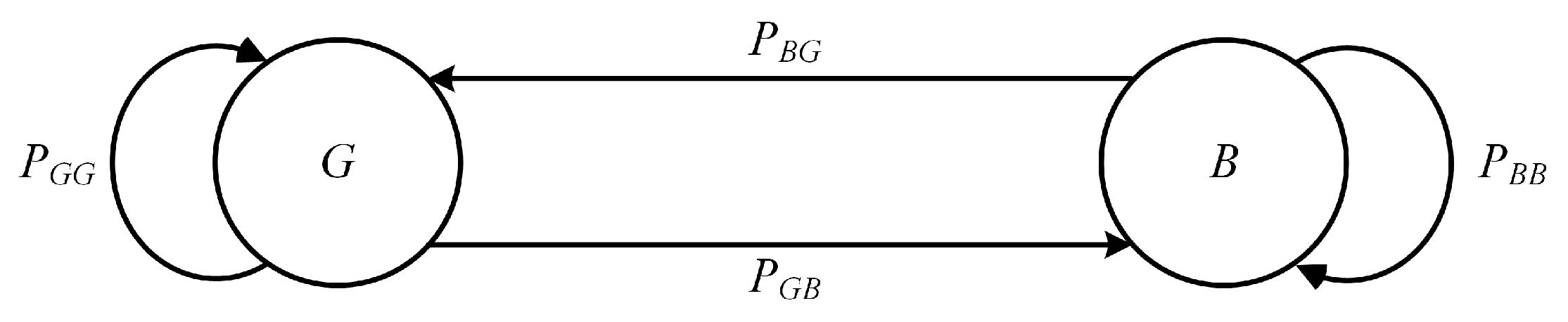
In order to model the bursty nature of impulsive noise, a Markov-Gaussian model was proposed in [5]. The following transition probability matrix,

$$\mathbf{P}=\left[\begin{array}{cc}{P}_{GG}& P_{GB}\\ P_{BG}& P_{BB}\end{array}\right],$$

(5)

accounts for the correlation between successive noise states. As in any transition matrix, the elements are such that $P_{GG}+P_{GB}=1$ and $P_{BG}+P_{BB}=1$, so that in the state diagram representation of the Markov-Gaussian noise, in Figure 1, the outgoing transition probabilities sum to one. Moreover, by introducing a correlation parameter $\gamma ={(P_{GB}+P_{BG})}^{-1}$, the steady-state probabilities of the two noise states are $P_G=\gamma P_{GB}$ and $P_B=\gamma P_{BG}$. The parameter $\gamma$ determines the amount of correlation between successive noise states, so that a larger $\gamma$ implies an increased burstiness of impulsive noise. More explicitly, the average duration of permanence in a given noise state is:

$$\begin{array}{c}\hfill T_B=\frac{\gamma }{P_B}{T}_G=\frac{\gamma }{P_G}\end{array}$$

(6)

whereas $T_B=P_B^{-1}$ and $T_G=P_G^{-1}$ would occur in the case of a memoryless Bernoulli-Gaussian process, to which the Markov-Gaussian model reduces in the case $\gamma =0$.

2.2. Markov Middleton Class A Noise

In this model, the number i of interferers, at time k, can exceed one and can be virtually any integer number, despite that a maximum number M of interferers is usually considered for practical reasons. The Gaussian interferers are all independent of each other and are assumed to have the same power, ${\sigma }_I^2$. As in the Bernoulli-Gaussian and in the Markov-Gaussian models of Section 2.1, the interferers are superimposed on an independent background noise sequence $\left\{n_k^G\right\}$ with variance ${\sigma }_G^2$, so that the overall noise power is ${\sigma }_i^2={\sigma }_G^2+i{\sigma }_I^2$, whenever the channel is in state i, i.e., i interferers are active. The pdf of noise samples is thus:

$$p\left(n_k\right)=\sum _{i=0}^{\infty }\frac{P_i}{\sqrt{2\pi {\sigma }_i^2}}\exp \left\{-\frac{n_k^2}{2{\sigma }_i^2}\right\}.$$

(7)

In the Middleton class A model, the channel state is assumed to follow a Poisson distribution [4], so that in (7), $P_i=e^{-A}{A}^i{(i!)}^{-1}$, where A is called the impulsive index and can be interpreted as the average number of active interferers per time unit. When the channel state accounts for i interferers, we can thus express the total noise power as:

$${\sigma }_i^2=\left(1+\frac{i}{A\Gamma }\right){\sigma }_G^2$$

(8)

in which a new parameter $\Gamma ={\sigma }_G^2{\left(A{\sigma }_I^2\right)}^{-1}$ represents the ratio between the power of background noise and the average power of interferers. The average power of Markov Middleton class A noise is thus:

$${\sigma }^2=E\left[{\sigma }_i^2\right]=\sum _{i=0}^{\infty }{\sigma }_i^2{P}_i=\left(1+\frac{1}{\Gamma }\right){\sigma }_G^2$$

(9)

In order to avoid the practical complications of an extremely large (and unlikely) number of interferers, by exploiting the rapidly decreasing values of the Poisson distribution, an approximation of the Middleton class A noise is usually introduced by truncating its pdf to a maximum value for the channel state $i\le M$, as follows:

$$p\left(n_k\right)=\sum _{i=0}^{M-1}\frac{P_i^{\prime }}{\sqrt{2\pi {\sigma }_i^2}}\exp \left\{-\frac{n_k^2}{2{\sigma }_i^2}\right\}\begin{array}{cc},& P_i^{\prime }=\frac{P_i}{{\sum }_{j=0}^{M-1}{P}_j}\end{array}.$$

(10)

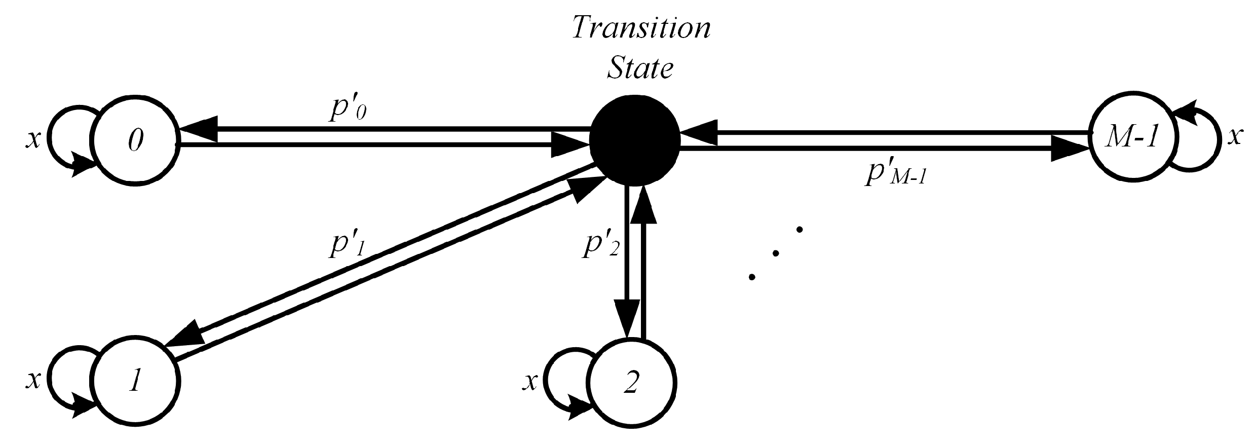
In order to account for memory in the Middleton class A model, a hidden Markov model (HMM) is assumed to govern the underlying transitions among channel states, so that successive noise states are correlated [6]. The corresponding transition probability matrix is thus:

$$P=\left[\begin{array}{cccc}x+(1-x)P_0^{\prime }& (1-x)P_1^{\prime }& \cdots & (1-x)P_{M-1}^{\prime }\\ (1-x)P_0^{\prime }& x+(1-x)P_1^{\prime }& \cdots & (1-x)P_{M-1}^{\prime }\\ ⋮& ⋮& ⋮& ⋮\\ (1-x)P_0^{\prime }& (1-x)P_1^{\prime }& \cdots & x+(1-x)P_{M-1}^{\prime }\end{array}\right],$$

(11)

in which each row sums to one and x is the correlation parameter. Referring to the state diagram in Figure 2, the channel can remain in the present state $i_k\in \{0,1,\cdots ,M-1\}$ with probability x or otherwise switch to one of the states (including $i_k$), with a (pruned, due to (11)) Poisson distribution. The average duration of an impulsive event with m interferers, i.e., the average permanence time within a state m, can be computed as:

$$T_m=\frac{1}{(1-x)(1-P_m^{\prime })}.$$

(12)

The Markov–Middleton class A model reduces to the simpler memoryless Middleton class A model in the case $x=0$. At the same time, the Markov-Gaussian model is an instance of the Markov–Middleton class A model, for $M=2$. Despite the latter being a more general model that includes the earlier, we illustrate and analyze both, in line with the existing literature that has developed along the two tracks.

In any case, the expression of noise samples to be considered in the observation model (1) is the one in (4).

3. Factor Graph and Sum-Product Algorithm

As a common technique to perform maximum a posteriori (MAP) symbol estimation, we use a factor graph representation for the variables of interest and for the relationships among them that stem from the system model at hand. These variables and relationships are in turn the variable nodes and the factor nodes appearing in the FG [18]. The aim is to compute the marginal distributions (pdf) of the random variables to be estimated, i.e., the transmitted signal samples $s_k$, conditioned on the observation of the received noisy samples $y_k$ in (1), whereas the overall FG represents the joint distribution of all the variable nodes, i.e., of transmitted samples, as well as of channel states $i_k$. Despite that this marginalization task is nontrivial, in the case of many (e.g., thousands of) variable nodes, it is brilliantly accomplished by the sum-product algorithm (SPA), which is a message passing algorithm able to reach the exact solution in the case of FGs without loops [18].

Thanks to Bayes’ rule, the joint posterior distribution of signal samples $\mathit{s}=\left\{s_k\right\}$ and channel states $\mathit{i}=\left\{i_k\right\}$ given the observation samples $\mathit{y}=\left\{y_k\right\}$ can be factorized as follows.

$$\begin{array}{cc}\hfill p(\mathit{s},\mathit{i}\mid \mathit{y})& \propto p(\mathit{y}\mid \mathit{s},\mathit{i})p\left(\mathit{s}\right)P\left(\mathit{i}\right)\hfill \\ \hfill & =\left[\prod _{k=1}^{K-1}p(y_k\mid s_k,i_k)p(s_k\mid s_{k-1})P(i_k\mid i_{k-1})\right]p(y_0\mid s_0,i_0)p\left(s_0\right)P\left(i_0\right).\hfill \end{array}$$

(13)

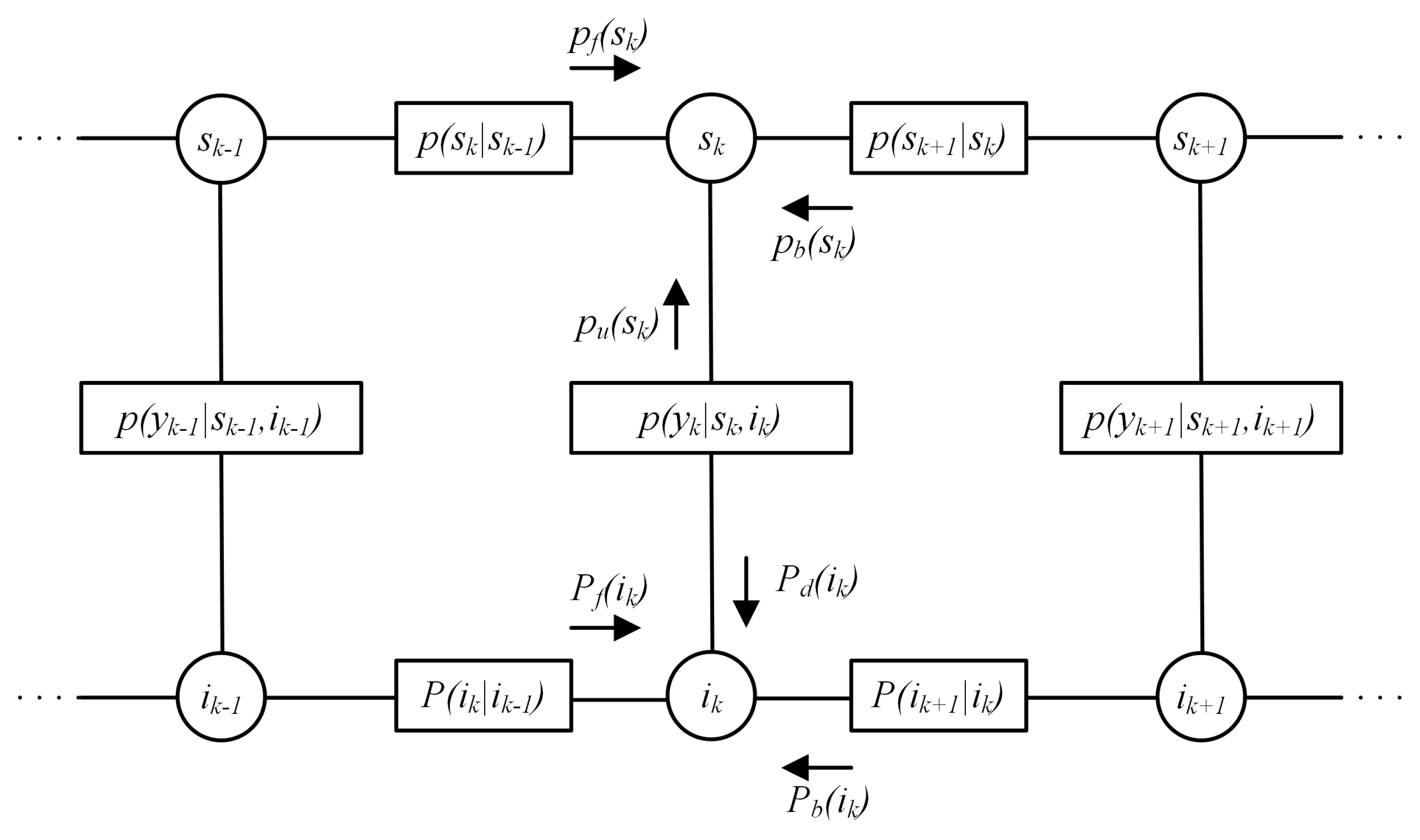
The Markovianity of both the signal sequence and of the noise sequence is a key factor in the application of the chain rule in (13), where simplified expressions result for its factors. Such a short-term memory (The Markov property of signal and noise sequences could be easily extended to a memory larger than one. This would however complicate the resulting notation without introducing an extra conceptual contribution.) implies that, besides the two types of variable nodes, i.e., $s_k$ and $i_k$, the FG consists of three types of factor nodes, i.e., $p(y_k\mid s_k,i_k)$, $p(s_k\mid s_{k-1})$, and $P(i_k\mid i_{k-1})$, the latter involving only pairs of time-adjacent variable nodes. This feature is further evidenced by the FG depicted in Figure 3, which graphically represents the joint pdf in (13). The pdfs $p(s_k\mid s_{k-1})$ and $p(y_k\mid s_k,i_k)$ and the conditional probability mass function (PMF) $P(i_k\mid i_{k-1})$ simply arise from the system model, i.e., from Equations (1), (2), and (5) or (11), and from the statistical description of the random variables therein. By denoting $g(x;\eta ,{\gamma }^2)$ the standard Gaussian pdf with mean $\eta$ and variance ${\gamma }^2$, we have:

$$\begin{array}{ccc}\hfill p(s_k\mid s_{k-1})& =& g(s_k;a_1{s}_{k-1},(1-a_1^2){\sigma }_s^2)\hfill \end{array}$$

(14)

$$\begin{array}{ccc}\hfill P(i_k\mid i_{k-1})& =& \mathit{P}(i_{k-1}+1,i_k+1)\hfill \end{array}$$

(15)

$$\begin{array}{ccc}\hfill p(y_k\mid s_k,i_k)& =& g(y_k;s_k,{\sigma }_{i,k}^2)\hfill \end{array}$$

(16)

where ${\sigma }_{i,k}^2={\sigma }_G^2+i_k{\sigma }_I^2$ is the variance of the observed sample at time k, which depends on the corresponding impulsive noise state $i_k$, represented by the variable node under the factor node (16), in Figure 3. In (15), the transition probability between successive impulsive noise states is found from the entries $\mathit{P}(i,j)$ of the matrix (5) or (11), depending on which of the noise models is adopted.

A straightforward application of the SPA [18] yields the forward and backward messages exchanged along the top line of the graph,

$$\begin{array}{ccc}\hfill p_f\left(s_k\right)& =& \int p_f\left(s_{k-1}\right)p_u\left(s_{k-1}\right)p(s_k\mid s_{k-1})d{s}_{k-1}\begin{array}{cc}& (k=1,\cdots ,K-1)\end{array}\hfill \end{array}$$

(17)

$$\begin{array}{ccc}\hfill p_b\left(s_k\right)& =& \int p_b\left(s_{k+1}\right)p_u\left(s_{k+1}\right)p(s_{k+1}\mid s_k)d{s}_{k+1}\begin{array}{cc}& (k=K-2,\cdots ,0)\end{array}\hfill \end{array}$$

(18)

where the initial condition for (17) is $p\left(s_0\right)=g(s_0;0,{\sigma }_s^2)$, while a constant value, as $p\left(s_{K-1}\right)=1$, is assumed to bootstrap the backward messages, which models the absence of a posteriori information on the last signal sample. In a similar way, the forward and backward messages exchanged along the bottom line of the FG are:

$$\begin{array}{ccc}\hfill P_f\left(i_k\right)& =& \sum _{i_{k-1}}P(i_k\mid i_{k-1})P_f\left(i_{k-1}\right)P_d\left(i_{k-1}\right)\begin{array}{cc}& (k=1,\cdots ,K-1)\end{array}\hfill \end{array}$$

(19)

$$\begin{array}{ccc}\hfill P_b\left(i_k\right)& =& \sum _{i_{k+1}}P(i_{k+1}\mid i_k)P_b\left(i_{k+1}\right)P_d\left(i_{k+1}\right)\begin{array}{cc}& (k=K-2,\cdots ,0)\end{array}.\hfill \end{array}$$

(20)

where the initial conditions clearly depend on the adopted noise model. In the Markov-Gaussian case, the pdf of the initial impulsive noise state is $p\left(i_0\right)=P{}_G\delta \left(i_0\right)+P_B\delta (i_0-1)$, while it is expressed as $p\left(i_0\right)={\sum }_{n=0}^{M-1}P{}_n^{\prime }\delta (i_0-n)$, in the case of Markov–Middleton noise, according to the descriptions in Section 2.1 and Section 2.2. In both cases, a uniform PMF (obtained by setting a possibly unnormalized equal value, as $P\left(i_{K-1}\right)=1$, for any of its realizations) models the absence of prior assumptions on the last impulsive noise state.

The upward and downward messages, on the vertical branches of the FG, are directed, respectively, towards the variable nodes $s_k$ and $i_k$ of our interest, and their expressions are:

$$\begin{array}{ccc}\hfill p_u\left(s_k\right)& =& \sum _{i_k}{P}_f\left(i_k\right)P_b\left(i_k\right)p(y_k\mid s_k,i_k)\begin{array}{cc}& (k=0,1,\cdots ,K-1)\end{array}\hfill \end{array}$$

(21)

$$\begin{array}{ccc}\hfill P_d\left(i_k\right)& =& \int p_f\left(s_k\right)p_b\left(s_k\right)p(y_k\mid s_k,i_k)d{s}_k\begin{array}{cc}& (k=0,1,\cdots ,K-1)\end{array},\hfill \end{array}$$

(22)

where, given the Gaussian expression (16), the integral in (22) takes the form of a convolution.

The described FG, as is evident from Figure 3, includes loops; hence, the SPA does not terminate spontaneously. As is well known, approximate variational inference techniques are required, in these cases [18]. We shall describe some of them in Section 4—including both traditional approaches and novel ones—and the performance of the resulting algorithms will be compared in Section 5. Nevertheless, all of them share a few fundamental features: (i) first, the resulting algorithms are all iterative, passing messages more than once along the same FG edge and direction; (ii) as a consequence, scheduling is a main issue, since it defines the message passing procedure; (iii) during iterations, the complexity of messages spontaneously tends to “explode”, so that clever message approximation strategies must be devised [18,19].

More specifically, regarding message approximations (Point iii) above), the usual approach is the following. Cast in qualitative parlance, one should: (1) select an approximating family, i.e., a family of pdfs/PMFs that is flexible and tractable enough, possibly exhibiting closure properties under multiplication, convolution, or other mathematical operations; (2) select an appropriate divergence measure to quantify the accuracy of the approximation, hence to identify the best approximating pdf within the chosen family [20]. While there is no standard method to select the approximating family, the most common choice for the divergence measure is the Kullback–Leibler (KL) divergence, for which we give a few details hereafter.

3.1. Kullback–Leibler Divergence

The KL divergence is an information theoretic tool (see, e.g., [20]) that can be used to measure the similarity between two probability distributions. We can search a pre-selected approximating family $\mathcal{F}$ of (possibly “simple”) distributions, to find the distribution $q\left(x\right)$ closest to a given distribution $p\left(x\right)$, which is possibly much more “complicated” than $q\left(x\right)$ (such as, e.g., a mixture). Such an operation is called projection and is accomplished by minimizing the KL divergence, as:

$$\mathrm{proj}\left[p\left(x\right)\right]=arg\underset{q\in \mathcal{F}}{min}\mathrm{KL}\left(p\left(x\right)\left|\right|q\left(x\right)\right).$$

(23)

A common choice is to let $q\left(x\right)$ belong to an exponential family, $q\left(x\right)=exp\left({\sum }_j{G}_j\left(x\right)v_j\right)$, where $G_j\left(x\right)$ are the so-called features of the family and $v_j$ are the so-called natural parameters of the distribution. Gaussian pdfs of Tikhonov pdfs, just to name a couple, are common distributions that naturally belong to exponential families, each with its own set of features ($G_j\left(x\right)=x^j$ ($j=0,1,2$) for the Gaussian; $G_1\left(x\right)=cos\left(x\right)$ and $G_2\left(x\right)=sin\left(x\right)$ ($j=1,2$) for the Tikhonov) and each with its own set of constraints on the natural parameters (e.g., $v_2<0$, for the Gaussians), which force the family to include proper distributions only. Exponential families have the pleasant property of being closed under the multiplication operation. Furthermore, it can be shown [20] that the projection operation in (23) simply reduces to equating the expectation of each feature with respect to the true distribution $p\left(x\right)$, $E_p\left[G_i\left(x\right)\right]$, with that computed with respect to the approximating distribution $q\left(x\right)$, $E_q\left[G_i\left(x\right)\right]$. Such a procedure of matching the expectations (of the features) is at the heart of (and gives the name to) the celebrated EP (expectation propagation) algorithm [21], further applied in Section 4 to our problem.

To get a better understanding of this procedure, let us apply it to project a Gaussian mixture onto a single Gaussian pdf. Suppose $p\left(x\right)$ is the following Gaussian mixture:

$$p\left(x\right)=\sum _i{\alpha }_{i}g(x;{\mu }_i,{\sigma }_i^2),$$

(24)

where ${\sum }_i{\alpha }_i=1$ for normalization. We shall approximate it by the nearest Gaussian $q\left(x\right)$ in the sense of the KL divergence, i.e., by applying (23). For that purpose, given that the expectations of the features of a Gaussian distributions are simply the mass, the mean, and the mean-squared value of that Gaussian (i.e., the expectations of one, x and $x^2$), the matching of these moments computed under $p\left(x\right)$ with those computed under $q\left(x\right)$ simply amounts to equating the mean and variance of the two distributions (assuming that both $p\left(x\right)$ and $q\left(x\right)$ are normalized).

$$\begin{array}{ccc}\hfill E_q\left[x\right]=E_p\left[x\right]& =& \sum _i{\alpha }_i{\mu }_i\hfill \end{array}$$

(25)

$$\begin{array}{ccc}\hfill E_q\left[x^2\right]=E_p\left[x^2\right]& =& \sum _i{\alpha }_i\left({\sigma }_i^2+{\mu }_i^2\right)\hfill \end{array}$$

(26)

are the resulting algebraic equations from which the parameters (both the natural parameters and the moments) of the best approximating Gaussian $q\left(x\right)$ are derived.

4. Signal Estimation

Referring to the FG in Figure 3, which models the problem described in Section 2, we shall first show that the message passing procedure that is established by the SPA, as detailed in Section 3, along the horizontal edges of the FG coincides with two classical estimation problems and is solved by two equally classical signal processing algorithms. Namely, along the top line of edges in the FG, the forward-backward message passing of Gaussian estimates for the (continuous) samples $s_k$ coincides with the celebrated Kalman smoother [24]. Along the bottom line of edges in the FG, a similar forward-backward message passing of (discrete) PMFs exactly follows the famous BCJR algorithm [25] (named after the initials of the authors), which is known to provide an MAP estimate of the channel states $i_k$ at each time epoch, i.e., for the variable nodes along the bottom line of the FG. It is significant that the same BCJR algorithm was recently implemented in [11], in the context of a problem similar to ours, where memoryless Gaussian signal samples were estimated in the presence of Markov-Gaussian impulsive noise (to which our system model reduces in the special case $a_1=0$ and $M=2$).

It is indeed the memory in both the signal and the noise sequences that makes the loopy FG in Figure 3 “unsolvable” (in the sense of marginalizing the joint pdf) with the SPA. The problem arises in fact from the messages passed along the vertical edges of the FG, i.e., those that connect the top half (that of signal samples) to the bottom one (that of impulsive noise channel states). As discussed in the following in more detail, while the downward messages (22) result from products and convolutions of Gaussian pdfs, hence themselves Gaussian, this is not the case for the upward messages in (21), which are Gaussian mixtures, basically due to the presence of the discrete variables $i_k$. That of mixed discrete and continuous variable nodes is a well-known scenario that makes the number of mixture elements, hence the complexity of messages, increase exponentially at every time step, so that mixture reduction techniques should be employed [19]. Mixture reduction can either be accomplished by making hard decisions on the impulsive noise channel states or otherwise by exploiting the soft information contained in the mixture messages $p_u\left(s_k\right)$, through more sophisticated approximation schemes [26].

4.1. Upper FG Half: Kalman Smoother

Suppose that the lower part of the FG sends messages $p_u\left(s_k\right)$ consisting of a single Gaussian distribution, with mean ${\widehat{s}}_{u,k}$ and variance ${\widehat{\sigma }}_{u,k}^2$,

$$p_u\left(s_k\right)=g(s_k;{\widehat{s}}_{u,k},{\widehat{\sigma }}_{u,k}^2).$$

(27)

Under this assumption and based on the SPA, the forward and backward Equations (17) and (18) along the upper line of the FG coincide with those of a Kalman smoother [18]. To compute the forward and backward messages, we assume that ${\eta }_f$ and ${\eta }_b$ are respectively the means of the Gaussian messages $p_f\left(s_k\right)$ and $p_b\left(s_k\right)$ and ${\sigma }_f^2$ and ${\sigma }_b^2$ are their variances. Equations (14), (17), and (27) yield:

$$\begin{array}{cc}\hfill p_f\left(s_k\right)& =\int g(s_{k-1};{\eta }_{f,k-1},{\sigma }_{f,k-1}^2)g(s_{k-1};{\widehat{s}}_{u,k-1},{\widehat{\sigma }}_{u,k-1}^2)\hfill \\ \hfill & ·g(s_k;a_1{s}_{k-1},(1-a_1^2){\sigma }_s^2)d{s}_{k-1}\hfill \\ \hfill & =g(s_k;{\eta }_{f,k},{\sigma }_{f,k}^2)\hfill \end{array}$$

(28)

in which ${\eta }_{f,k}$ and ${\sigma }_{f,k}^2$ can recursively be updated as:

$$\begin{array}{ccc}\hfill {\eta }_{f,k}& =& a_1{\eta }_{f,k-1}+a_1\frac{{\sigma }_{f,k-1}^2}{{\sigma }_{f,k-1}^2+{\widehat{\sigma }}_{u,k-1}^2}({\widehat{s}}_{u,k-1}-{\eta }_{f,k-1})\hfill \end{array}$$

(29)

$$\begin{array}{ccc}\hfill {\sigma }_{f,k}^2& =& (1-a_1^2){\sigma }_s^2+a_1^2\frac{{\sigma }_{f,k-1}^2}{{\sigma }_{f,k-1}^2+{\widehat{\sigma }}_{u,k-1}^2}{\widehat{\sigma }}_{u,k-1}^2\hfill \end{array}$$

(30)

In the same way, the backward recursion can be obtained from (14), (18), and (27):

$$\begin{array}{cc}\hfill p_b\left(s_k\right)& =\int g(s_{k+1};{\eta }_{b,k+1},{\sigma }_{b,k+1}^2)g(s_{k+1};{\widehat{s}}_{u,k+1},{\widehat{\sigma }}_{u,k+1}^2)\hfill \\ \hfill & ·g(s_{k+1};a_1{s}_k,(1-a_1^2){\sigma }_s^2)d{s}_{k+1}\hfill \\ \hfill & =g(s_k;{\eta }_{b,k},{\sigma }_{b,k}^2)\hfill \end{array}$$

(31)

where:

$$\begin{array}{ccc}\hfill {\eta }_{b,k}& =& \frac{1}{a_1}{\eta }_{b,k+1}+\frac{1}{a_1}\frac{{\sigma }_{b,k+1}^2}{{\sigma }_{b,k+1}^2+{\widehat{\sigma }}_{u,k+1}^2}({\widehat{s}}_{u,k+1}-{\eta }_{b,k+1})\hfill \end{array}$$

(32)

$$\begin{array}{ccc}\hfill {\sigma }_{b,k}^2& =& \frac{1}{a_1^2}(1-a_1^2){\sigma }_s^2+\frac{1}{a_1^2}\frac{{\sigma }_{b,k+1}^2}{{\sigma }_{b,k+1}^2+{\widehat{\sigma }}_{u,k+1}^2}{\widehat{\sigma }}_{u,k+1}^2\hfill \end{array}$$

(33)

Thus, the message sent from the variable node $s_k$ to the factor node $p(y_k\mid s_k,i_k)$, here named $p_d\left(s_k\right)$, is Gaussian as well,

$$p_d\left(s_k\right)=p_f\left(s_k\right)p_b\left(s_k\right)=g(y_k;{\widehat{\eta }}_k,{\widehat{\gamma }}_k^2)$$

(34)

where, as in all Gaussian product operations, the variance and mean,

$$\begin{array}{ccc}\hfill {\widehat{\gamma }}_k^{-2}& =& {\sigma }_{f,k}^{-2}+{\sigma }_{b,k}^{-2}\hfill \end{array}$$

(35)

$$\begin{array}{ccc}\hfill {\widehat{\gamma }}_k^{-2}{\widehat{\eta }}_k& =& {\sigma }_{f,k}^{-2}{\eta }_{f,k}+{\sigma }_{b,k}^{-2}{\eta }_{b,k},\hfill \end{array}$$

(36)

are found by summing the precision (i.e., the inverse of the variance) and the precision weighted mean.

4.2. Lower FG Half: BCJR

As mentioned earlier, the message $P_d\left(i_K\right)$ in (22) is the result of a convolution between two Gaussian pdfs, one provided by the channel observation, $p(y_k\mid s_k,i_k)$, and the other, $p_d\left(s_k\right)$, by the upper FG half:

$$\begin{array}{cc}\hfill P_d\left(i_k\right)& =\int p_d\left(s_k\right)p(y_k\mid s_k,i_k)d{s}_k\hfill \\ \hfill & =\int g(s_k;{\widehat{\eta }}_k,{\widehat{\gamma }}_k^2)g(y_k;s_k,{\sigma }_{i,k}^2)d{s}_k\hfill \\ \hfill & =g(y_k;{\widehat{\eta }}_k,{\widehat{\gamma }}_k^2+{\sigma }_{i,k}^2).\hfill \end{array}$$

(37)

As discussed in Section 2.2, ${\sigma }_{i,k}^2$ takes M different values, each in a one-to-one correspondence with an impulsive noise channel state. According to (15) and (37), the forward and backward recursions (19) and (20), along the bottom line of the FG edges, are:

$$\begin{array}{cc}\hfill P_f\left(i_k\right)& =\sum _{i_{k-1}}P(i_k\mid i_{k-1})P_f\left(i_{k-1}\right)g(y_{k-1};{\widehat{\eta }}_{k-1},{\widehat{\gamma }}_{k-1}^2+{\sigma }_{i,k-1}^2)\hfill \end{array}$$

(38)

$$\begin{array}{cc}\hfill P_b\left(i_k\right)& =\sum _{i_{k+1}}P(i_{k+1}\mid i_k)P_b\left(i_{k+1}\right)g(y_{k+1};{\widehat{\eta }}_{k+1},{\widehat{\gamma }}_{k+1}^2+{\sigma }_{i,k+1}^2).\hfill \end{array}$$

(39)

The above equations form the well-known MAP symbol detection algorithm known as BCJR [25] and more generally referred to as the forward-backward algorithm [18].

For each variable node $i_k$, the product of (38) and (39) is the message, here named $P_u\left(i_k\right)$, that is sent upward to the factor node $p(y_k\mid s_k,i_k)$,

$$P_u\left(i_k\right)=P_f\left(i_k\right)P_b\left(i_k\right),$$

(40)

and can be regarded as a provisional estimated PMF for the M possible different values of the impulsive noise channel state.

4.3. Hard Decisions and the Parallel Iterative Schedule Algorithm

Substituting (16) and (40) in (21), it is clear that the resulting message:

$$p_u\left(s_k\right)=\sum _{i_k}{P}_u\left(i_k\right)g(y_k;s_k,{\sigma }_{i,k}^2)$$

(41)

is a Gaussian mixture and not a single Gaussian distribution, as assumed in (27).

The generation of a Gaussian mixture, at every vertical edge of the FG, exponentially increases the computational complexity. Thus, the use of mixture reduction techniques is unavoidable. For that purpose, one radical approach is to make a hard decision on every ${\widehat{i}}_k=\mathrm{argmax}\left\{\widehat{P}\left(i_k\right)\right\}$, selected as the modal value of the estimated PMF, $\widehat{P}\left(i_k\right)=P_u\left(i_k\right)P_d\left(i_k\right)$. The mixture (41) is thus approximated by its most likely Gaussian term, so that the assumption of having Gaussian priors for each $s_k$ (i.e., the information on the individual sample that does not depend on the correlated sequence), as carried by the upward messages $p_u\left(s_k\right)$, is respected and the algorithm in Section 4.1 can be applied.

With this approximation, we can then establish a “parallel iterative schedule” (PIS) in the loopy FG. The upper and lower parts of the FG work in parallel, at every iteration, according to their forward-backward procedure (corresponding, as seen, to the Kalman smoother and the BCJR, respectively). At the end of a forward-backward pass, the two halves of the FG exchange information through messages sent along the vertical edges of the graph. Namely, $p_d\left(s_k\right)$ is convolved with the corresponding Gaussian observation (16), so as to get $P_d\left(i_k\right)$ in (22), while $P_u\left(i_k\right)$ is used to update the impulsive noise state PMF, $\widehat{P}\left(i_k\right)=P_u\left(i_k\right)P_d\left(i_k\right)$, hence the estimated ${\widehat{i}}_k$, at every iteration. Such a scheduling and the approximate hard decision strategy, which is an essential part of it, shall guarantee the convergence of the overall iterative algorithm, as shown in Section 5.

4.4. Soft Decisions: EP and TP Algorithms

Hard decisions on every $i_k$ imply that only one part of the information, provided by the lower FG half (Section 4.2), is being used by the signal estimation, in the upper FG half (Section 4.1), and the rest of the information is being discarded. This is clearly a suboptimal approach.

A better performing soft information strategy can instead be pursued, based on approximating the mixture (41) by minimizing the KL divergence. This can be implemented by using either the EP algorithm or the TP algorithm. To have a better insight into the similarities and differences between EP and TP, considering the posterior marginal $p\left(s_k\right|\mathbf{y})$ obtained, according to the SPA rules, as the product of all incoming messages to the variable node $s_k$:

$$p\left(s_k\right|\mathbf{y})=p_f\left(s_k\right)p_b\left(s_k\right)p_u\left(s_k\right)=p_d\left(s_k\right)p_u\left(s_k\right),$$

(42)

where $p_d\left(s_k\right)$ in (34) is Gaussian and $p_u\left(s_k\right)$ in (41) is a Gaussian mixture; thus, $p\left(s_k\right|\mathbf{y})$ is a Gaussian mixture as well. An approximation for it can be computed by the projection operation (23), once an approximating exponential family $\mathcal{F}$ is selected. In the problem that we analyze in this manuscript, the Gaussian family seems a natural choice, so that:

$${\tilde{p}}^{EP}\left(s_k\right|\mathbf{y})=\mathrm{proj}\left[p_d\left(s_k\right)p_u\left(s_k\right)\right]=g(s_k;{\widehat{s}}_k,{\widehat{\sigma }}_k^2).$$

(43)

This is exactly the approach of the EP algorithm: the posterior marginal is approximated by matching the moments of the approximating Gaussian to those of the mixture, as discussed in Section 3.1, and the upward message $p_u\left(s_k\right)$, sent to the variable node $s_k$ for the next iteration, is replaced by the following, obtained by Gaussian division:

$$p_u^{EP}\left(s_k\right)=\frac{{\tilde{p}}^{EP}\left(s_k\right|\mathbf{y})}{p_d\left(s_k\right)}=g(s_k;{\widehat{s}}_{u,k}^{EP},{\left({\widehat{\sigma }}_{u,k}^{EP}\right)}^2).$$

(44)

$${\tilde{p}}^{TP}\left(s_k\right|\mathbf{y})=p_d\left(s_k\right)p_u^{TP}\left(s_k\right),$$

(45)

to finally get the TP symbol estimate from the posterior marginal (45).

This division of pdfs, which is inherent to the EP algorithm, is not painless and can give rise to improper distributions, which in turn introduce instabilities into the algorithm [21,26,27]. This is easily understood by considering a Gaussian division in (44) where the variance of the denominator is larger than the variance of the numerator, so that an absurd negative variance results. Several techniques have been proposed to avoid these instabilities; we adopt the simple improper message rejection discussed in [27].

An alternative approach, which spontaneously avoids instabilities, is that of the TP algorithm [22], where it is the individual message $p_u\left(s_k\right)$, i.e., the mixture, that is projected onto an approximating (here Gaussian) pdf, instead of the posterior marginal, as done in EP:

$$p_u^{TP}\left(s_k\right)=\mathrm{proj}\left[p_u\left(s_k\right)\right]=g(s_k;{\widehat{s}}_{u,k}^{TP},{\left({\widehat{\sigma }}_{u,k}^{TP}\right)}^2).$$

(46)

In TP, the posterior marginal, from which the signal sample is estimated, is as usual obtained by multiplying the incoming messages to $s_k$, i.e., the TP message (46) is multiplied by $p_d\left(s_k\right)$:

Note that the result in (46) would be obtained from the EP projection in (44) if only the operator $\mathrm{proj}[·]$ in (43) were transparent to $p_d\left(s_k\right)$, i.e., if it were $\mathrm{proj}\left[p_d\left(s_k\right)p_u\left(s_k\right)\right]=p_d\left(s_k\right)\mathrm{proj}\left[p_u\left(s_k\right)\right]$ (which amounts to stating ${\tilde{p}}^{EP}\left(s_k\right|\mathbf{y})={\tilde{p}}^{TP}\left(s_k\right|\mathbf{y})$), which is in general not the case. Finally, the TP algorithm is inherently stable and does not require any complementary message rejection procedure.

5. Results

We evaluated, by numerical simulation, the mean-squared error (MSE) versus the average signal-to-noise ratio (SNR) in a bursty impulsive noise scenario with a maximum of $M-1$ interferers, i.e., with M noise states, where the zeroth state corresponds to background noise only. As discussed in Section 2, the peculiarity of this system is that the actual ratio of signal-to-noise power can dramatically change at every time epoch.

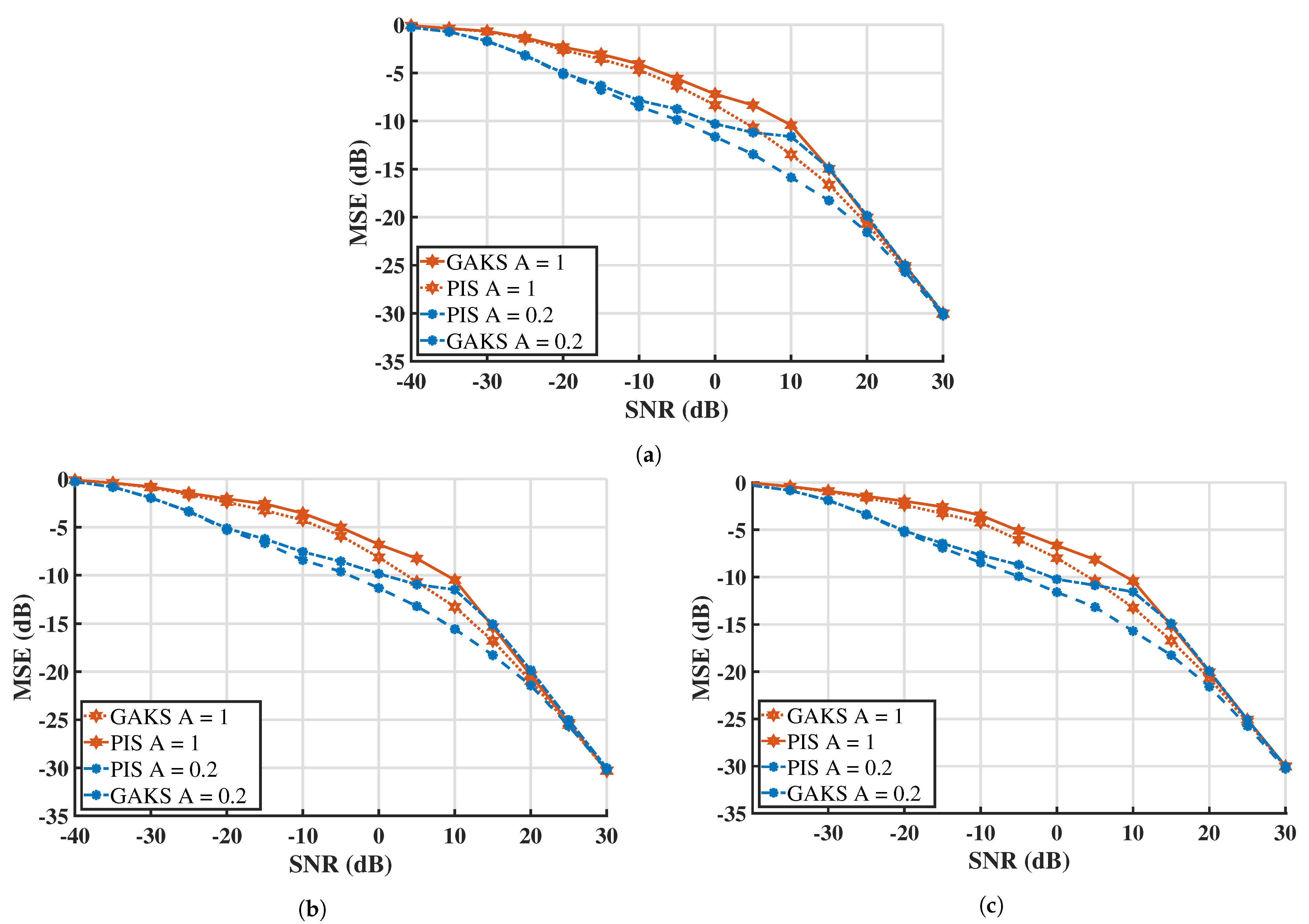
Figure 4 shows the MSE for the estimated signals corrupted by impulsive noise with $M=2,4,16$ states (Figure 4a–c), where the following system parameters were chosen for the simulation. The correlation parameter x was set to $0.9$, meaning that the channel state is expected to switch to a new state (including the present one) with probability $0.1$; adjacent noise samples are thus highly correlated, i.e., the noise is bursty. The impulsive index A, i.e., the average number of active interferers, was chosen to be either $0.2$ or one, which statistically corresponds to a “hardly present interferer” or to an “almost constantly present” one (at least). $\Gamma$ is the ratio between the power of background noise and the average power of interferers and was set to $0.01$, corresponding to a strongly impulsive noise where interference can boost noise power by a factor of ${\Gamma }^{-1}=100$. The signal parameters, in the AR(1) model, were set as follows: $a_1=0.9$ and ${\sigma }_s^2=1$ (i.e., normalized signal power). We transmitted 100 frames of 1000 samples each (for a total number of ${10}^5$ received samples).

The curve labeled GAKS in Figure 4 shows the performance of a “genie-aided Kalman smoother” and refers to an ideal receiver with perfect channel state information, i.e., with exact knowledge of $i_k$, hence of noise variance at every time epoch. In this case, the system reduces to the classical estimation of correlated Gaussian samples, for which the Kalman smoother is optimal; hence, the GAKS curve represents a lower bound for the performance of any non-ideal receiver. The curve labeled PIS in Figure 4 is obtained through the parallel iterative schedule algorithm discussed in Section 4.3.

A comparison of Figure 4a–c reveals that the simulation results are very close to each other. A fine checking of the numerical values reveals, for example, that in the $M=2$ case of Figure 4a, at SNR = $-5$ dB, the MSE is $-5.598$ dB for $A=1$ and $-8.763$ dB for $A=0.2$. In the $M=4$ case of Figure 4b, at the same SNR values, the MSE changes to $-5.038$ and $-8.573$, while in the $M=16$ case of Figure 4c, the MSE values change to $-5.103$ and $-8.708$. This implies that the performance of the estimator is not considerably changed when we opt for noise models with more than $M=2$ states, which corresponds to the Markov-Gaussian model of Section 2.1. The reason is that a larger maximum number of interferers implies a smaller amount of power per interferer, so that, for a given average SNR, it is the average number of active interferers A, rather than its maximum value $M-1$, that determines the performance. Results in Figure 4 confirm, as expected, that a larger A degrades the performance of the estimator.

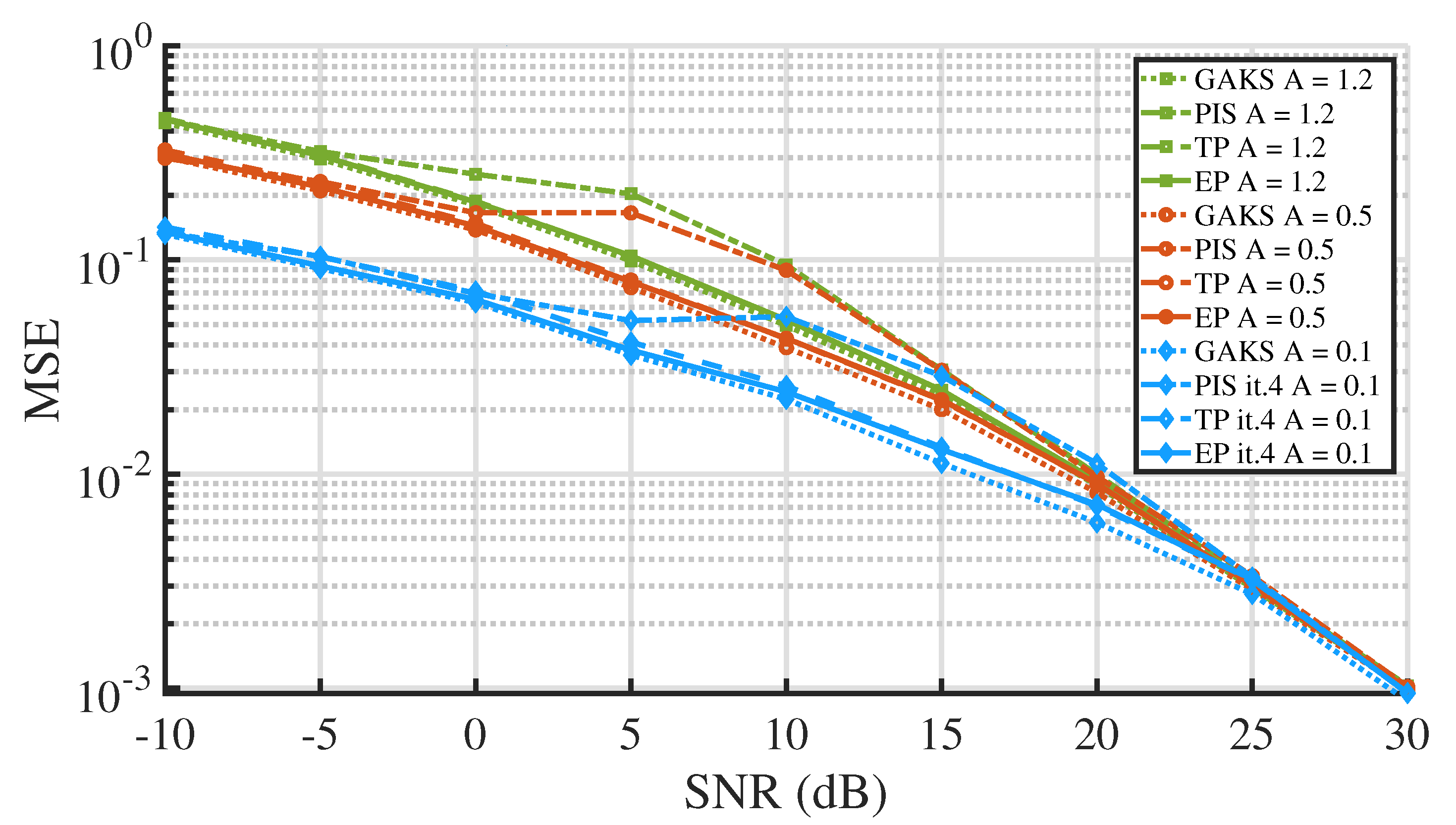
For this reason, in the following simulations, we limited our attention to the case $M=4$ only. We considered the same noise parameters as in [6], i.e., a correlation parameter $x=0.98$, corresponding to an impulsive noise with increased burstiness, while the values of $A=0.2$ or $0.8$ were slightly decreased (compared to Figure 4). The values $\Gamma =0.01$ and $0.001$, considered in Figure 5a,b, account for a strongly impulsive noise, where the impulsive events can increase the noise power up to 1000 times the background noise power.

Figure 5 shows the performance of an estimator that implements the EP and TP algorithms described in Section 4.4 (curves labeled EP and TP) that pursue the approximation of Gaussian mixture messages. These strategies exploit soft decisions on the impulsive noise states and show a superior performance, compared to the PIS algorithm, which is based on hard decisions on $i_k$. As can be seen in Figure 5, the performance of PIS is degraded especially around SNR values where the signal and noise power are balanced. At these SNR levels (0–10 dB), signal estimation is neither dominated by noise, nor is it similar to a noiseless scenario. On the contrary, the performance of both EP and TP is close to the lower bound (GAKS), meaning that these algorithms are practically optimal. If we do not consider the issue of convergence, it would thus be irrelevant to choose either of the two. However, we recall that the EP algorithm requires the implementation of an extra improper message rejection strategy. In contrast, the TP algorithm is inherently stable and requires less computations, and it is thus the preferable choice, for this problem.

A comparison between Figure 5a,b further proves that the performance of the estimator does not strongly depend on the value of $\Gamma$, as one could expect. To complete the picture, Figure 6 reports simulation results obtained at other different impulsive index values ($A=0.1,0.5,1.2$). The MSE values in Figure 5a and Figure 6 definitely show that it is the impulsive index A that dictates the system performance. The two values $A=0.2$ and $0.8$ considered in Figure 5a are associated with curves that fit in between those in Figure 6, which are associated with the other three values of A. For each value of A, the EP and TP algorithms provide results almost coinciding with the lower bound (GAKS), while the PIS algorithm entails a consistent loss in performance, especially at intermediate SNR values (5–10 dB).

The iterative algorithms that were analyzed (PIS, EP, TP) showed a fast convergence in all cases, so that simulations were carried out in four iterations; we verified that convergence is practically reached in three iterations and that no further modification of results occurs after the fourth iteration (as we tested, until the 10th iteration).

6. Conclusions

We proposed different algorithms to estimate correlated Gaussian samples in a bursty impulsive noise scenario, where successive noise states are highly correlated. The receiver design was based on a factor graph approach, resulting in a loopy FG due to the correlation among signal samples, as well as among noise samples [18]. Due to the joint presence of continuous and discrete random variables (namely, signal samples and impulsive noise channel states), as typically occurs in these cases, the resulting iterative sum-product algorithm has an intractable complexity [20]. The bursty impulsive noise is in fact modeled either as Markov-Gaussian [5] or as Markov–Middleton [6]; hence, the channel is characterized by (dynamically switching) states that count the sources of electromagnetic interference, at every time epoch [4].

Although belonging to the broad class of switching linear dynamical systems [19], the system considered here exhibits remarkable symmetry properties that allow an effective estimation of the signal samples through approximate variational inference. A simple parallel iterative schedule (PIS) of messages, including dynamically updated hard decisions on the channel states [16], was shown to provide a satisfactory, although suboptimal, performance, for many different channel conditions [17]. The more computationally costly expectation propagation (EP) [21] is also applicable to this problem albeit affected by its usual instability problems during the iterations, which can however be solved by known methods in the literature [27]. For this reason, an alternative transparent propagation (TP) algorithm was introduced, which has a lower computational complexity (compared to EP) and is inherently stable [22]. Both EP and TP reach a performance that is close to the optimal one, i.e., that of a receiver with perfect channel state information.

For the first time, we applied all of these algorithms to bursty impulsive noise channels with a very large number (up to 15) of independently switching interferers [23]. The results demonstrate that, for a given SNR, the degradation induced by many (e.g., 15) interferers, with limited power, is similar to that produced by fewer (e.g., three) stronger interferers with correspondingly larger power. Hence, few-state channel models, or even the binary Markov-Gaussian model, are adequate to predict the performance with any of the algorithms discussed here, both suboptimal (PIS) and close to optimal (EP,TP).