Automatic Outdoor Patrol Robot Based on Sensor Fusion and Face Recognition Methods

Abstract

This study integrates path planning, fuzzy theory, neural networks, image processing, range sensors, webcam, global navigation satellite system (GNSS), and real-time kinematic (RTK) positioning system into an intelligent wheeled mobile robot (WMR) for outdoor patrolling. The robot system uses ultrasound sensors, laser sensors, and fuzzy controllers to detect obstacles and avoid them. The starting position and the goal position of the WMR in an outdoor environment are given by the GNSS RTK positioning system. Real-time position correction of the robot is performed through the differential global positioning system. The robot system applies the ant algorithm and the Dijkstra algorithm to find the shortest path for patrol tasks. The convolutional neural network image processing is utilized to identify intruders that are appearing in the patrol path. When the WMR detects an intruder by the face detection and recognition methods, the robot captures the photo of this person by the webcam and acquires the location information of this person by the RTK positioning system. Then the WMR sends the location and photo of the intruder to the control center by Wi-Fi and asks for help.

1. Introduction

Starting in 2019, with the rapid spread of Coronavirus disease (COVID-19), governments all over the world have called on people to isolate themselves at home, or even stop going to work. Therefore, when people are unable to work for various reasons, how to make automatic machinery or intelligent robots continue to work instead of human labor and let the world continue to run is currently an important goal and research issue. Robots of different types have been developed based on different requirements. Most intelligent robots integrate automation, control, electronics, mechanics, and communication technologies. The expensive intelligent robot system integrates many advanced technologies and theories such as path planning [1], image processing, obstacle avoidance technology [2], arms control [3], navigation [4], and so on. Those technologically advanced robots are usually expensive and difficult to maintain. However, a robot structure that is cheap and simple in design needs to be developed to completely replace human labor, and despite being beneficial to the whole world, this is a challenging task. After the outbreak of the pandemic, many tasks need robots that can replace humans, such as simple material transportation and environmental patrol. However, the goal is to design and develop this kind of robot that is easy to manufacture, assemble and repair, and it should be relatively cheap and practical, and although this is challenging to achieve and there is still a lot of room for improvement so far.

Our lives have become troubled by the current pandemic, and when the outdoor air is no longer safe, robots are needed to replace humans in outdoor patrols. Wheeled mobile robots (WMR) are the commonly used robots in many applications. The advantages of the WMR include easy control and fast movement, therefore, the WMR was used in this study. Omnidirectional WMR has more advantages than a normal directional wheeled mobile robot, such as mode of action, easy control, and high mobility [5,6,7,8]. Therefore, to design an intelligent control system that replaces human labor and make the WMR able to independently assist human patrol in an outdoor environment is the primary research motivation of this study. Since the late 1990s, many papers have been presented regarding robot outdoor patrol [9,10,11,12,13]. These studies mainly focused on navigation, obstacle avoidance, path planning, road detection, and object recognition. Intruder identification and location informing were not included. Here, we put focus on fast path planning and fast face recognition. In addition, a new function of intruder alert is added.

There have been many research efforts devoted to the problem of robot path planning, such as the Dijkstra algorithm, A* algorithm, and ant algorithm [14]. For obstacle avoidance, among most studies, the majority use fuzzy controllers to control WMR [15]. For detecting obstacles, there are many kinds of sensors, such as infrared sensors, ultrasonic sensors, and laser sensors that can be used to detect obstacles. This study integrates the global navigation satellite system real-time kinematic (GNSS RTK) positioning system, laser sensor, Dijkstra algorithm, ant algorithm, fuzzy controller, CNN [16] image processing, ultrasound sensors, and webcam into an intelligent robot system to perform outdoor patrol. The laser sensor, ultrasound sensors, and fuzzy controller are applied to detect and avoid obstacles. The starting position and the goal position of the WMR in an outdoor environment are given by the GNSS RTK positioning system. The robot system uses the Dijkstra algorithm with ant algorithm to find the shortest path for patrol tasks. In the outdoors, the robots may move to an unknown environment. Therefore, a navigation system installed on the robot is particularly important, so that the robot can know the current location and check whether it reaches the destination or not. Path planning is another important issue of robot research. Path planning allows the robot to move as much as possible on a shorter and collision-free path. Image processing is used to detect any intruder who appears on the patrol path. If the WMR detects a stranger by the face detection and recognition methods, it will capture the photo of this person by a webcam and get the location information of this person by the positioning system. Then, the WMR will send the location and photo of the stranger to the control center by Wi-Fi and ask for help.

Robotic systems consist of different technologies. Many researchers have presented their studies of intelligent robot control. Huang utilized inverse kinematics of the D-H coordinate system in robot arm control [17], where the value of the robot joint variables can be determined according to the given position and posture of the end effector. Lian [18] used a fuzzy controller to control an obstacle avoidance mobile robot and made the robot have an adaptive intelligent obstacle avoidance system. The kinematic model of omnidirectional WMR was analyzed by Chung [19] to obtain a mobile system that does not require a radius of gyration. Aman et al. [20] presented an efficient sensor fusion method. The result is that different sensor fusion methods can be used to detect the size and location of obstacles. Then, Fukai et al. [21] used the TOF (Time of Flight) type range sensor to measure the distance, and then use that distance information acquired by the TOF camera to detect obstacles. The distance between the sensor and the object can be measured according to the time difference between signal emission and return, thereby improving the accuracy of 3D recognition. Leow combined kinematic models on a wheeled mobile robot [22], and constructed a very good modeling and nonlinear controller design for an omnidirectional mobile robot. Lin implemented obstacle avoidance and ZigBee control functions for omnidirectional mobile robots [23]. Zigbee is a low-power, low data rate, and close proximity (i.e., personal area) wireless ad hoc network. The results provide the FPGA implementation techniques for omnidirectional mobile robot control and extend the ZigBee wireless communication techniques into the intelligent robot research. Zhang et al. [24] proposed a hybrid method based on the A* algorithm and genetic algorithm to solve the problem of the optimum path planning for mobile robots. The authors used a GA approach for efficiently finding an (or near) optimal path in a grid map. GA is able to find the optimal paths in large environments equally to A* algorithm in all the simulated cases. Fadzli et al. [25] proposed a multi-layer dictionary storage structure for the Dijkstra algorithm. When applied to a map of any indoor terrain, the proposed method produced the most optimal path between two points. Kho et al. [26] installed the Global Positioning System (GPS) on an automated robot. GPS is used to determine position coordinates, time, and the default position of the robot and can map the shortest path for the robot to reach its goal from its current position. North et al. [27] proposed a system that integrates odometry from wheel encoders, low-cost MEMS-based inertial sensors, and GPS. During GPS outages, the Kalman Filter with velocity update derived from the forward speed from wheel encoders is a good technique for reducing localization errors. Mahendran and Vedaldi [28] showed that several layers in CNNs retain photographically accurate information about the image, with different degrees of geometric and photometric invariance. Shuyun et al. [29] proposed an improved ant colony optimization, and the global path planning of the robot is carried out based on the known two-dimensional environment map. Shuyun et al. designed a handling robot system that can recognize ribbons and signposts, and automatically charge [30]. Parada-Salado et al. [31] proposed the design and construction of a land-wheeled autonomous mini-robot (LWAMR) for indoor surveillance. Isakhani et al. [32] presented a local optimization navigation algorithm based on fuzzy logic, using the “recognition-memory” strategy to process the sensor information. When the current planning path forms a dead zone and runs repeatedly, “identification” is formed, and the path and navigation decision are re-planned to avoid obstacle colliding. In our study, the advantages of GPS, Dijkstra algorithm, ant algorithm, CNN, and fuzzy control are utilized in the control system design.

Contributions of this research are mainly in three parts. The first is to develop a robot that can conduct outdoor mobile patrols using a simple physical mechanical structure and inexpensive and easily available electronic components and motors. Secondly, a convolutional neural network in the system integration is used to improve the robot’s face recognition ability in outdoor patrol. Through the combination of Gaussian function a new type of ideal fuzzy control model is established. The DGPS method plus Dijkstra algorithm and ant algorithm for robot patrol in real-time path planning has been approved to be sufficiently accurate. Finally, through software integration and data transmission and analysis, a control center for remote robot manipulation and monitoring of patrol conditions can be set up anywhere, which proves the flexibility and feasibility of this conceptual system.

2. Materials and Methods

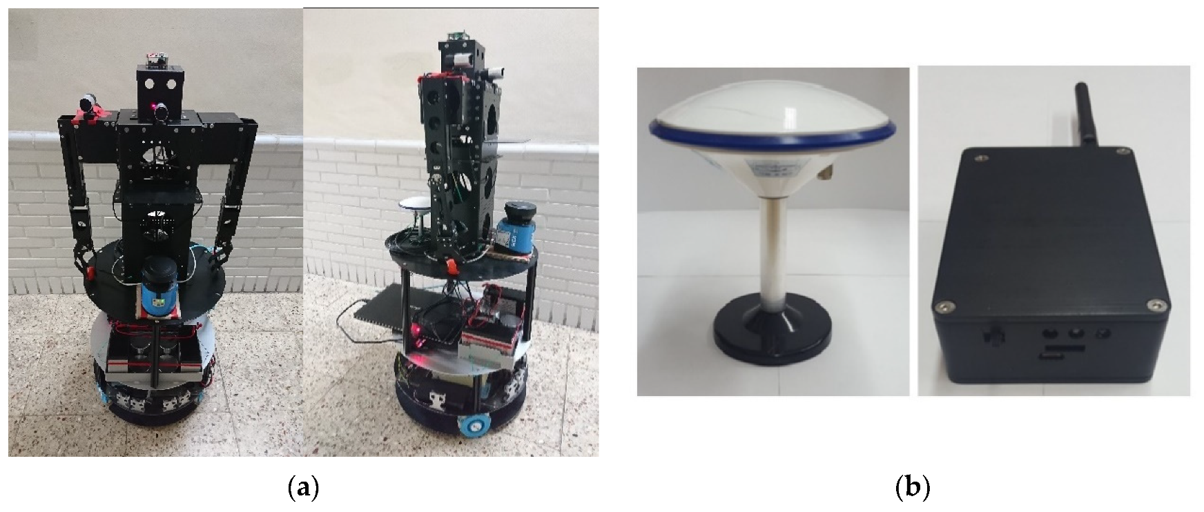
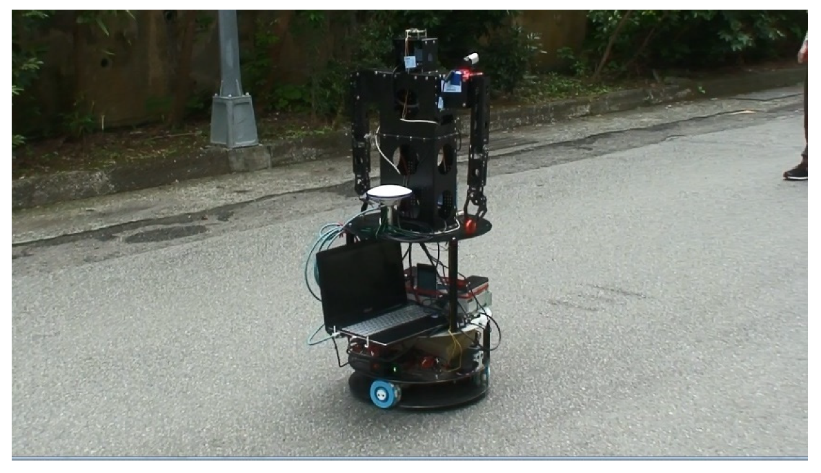
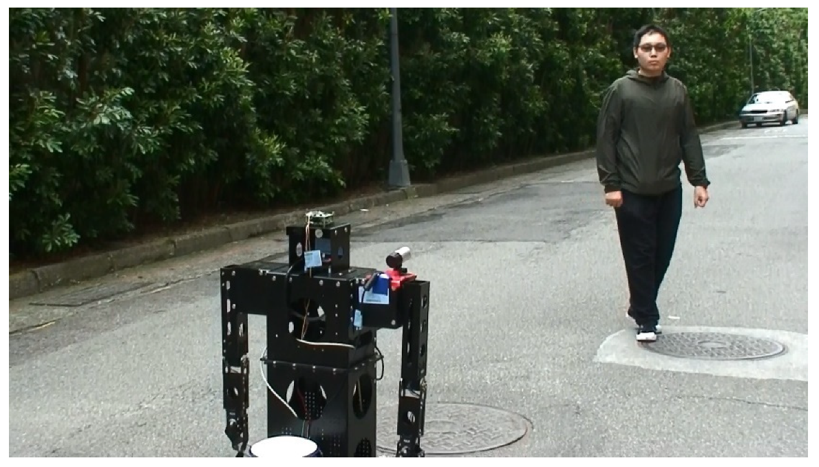
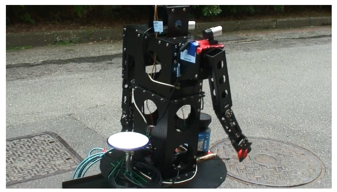
2.1. Composition and Structure of the Robot

The proposed control scheme is performed through experiment verification by an omnidirectional WMR robot. The size of the robot is 600 mm in length, 400 mm in width, and height is 850 mm, as shown in Figure 1a. The robot has six MX motors. The arms have two MX-64 motors in the shoulders, two MX-64 motors in the elbows, and two MX-28 motors at wrists on both sides. The MX-28 is 35.6 mm in length, 35.5 mm in width, and 50.6 mm in height. Its static torque is 2.5 N.m. The MX-64 is 40.2 mm in length, 41 mm in width, and 61.1 mm in height. Its static torque is 6.0 N.m. The robot has two mechanical arms and fingers that can grip objects, the length is 470 mm and 150 mm, respectively. The StarGazer is on top of the robot’s head for indoor navigation and position. The omnidirectional WMR’s chassis size is 240 mm radius. Three omnidirectional wheels are configured in separated 120° from each other, and three 12V-DC motors are installed to provide rated torque 700 g-cm. The WMR has two 12V batteries (12V1.3AH/20HR lead-acid batteries) and a UPS uninterruptible power system on the first and second layer. The WMR has six ultrasonic sensors in front of the carrier of the second layer, which is used to measure the distance of the obstacle. The WMR also has a SICK LMS100 2D laser scanner in front of the carrier of the fourth layer, which is used for long-distance measurements. Both sensors are used to detect an obstacle as well as to an avoid obstacle. The WMR has a GNSS RTK positioning system receiver in the back of the fourth layer, which is used for outdoor navigation and positioning. The GNSS RTK system consists of two parts, one is GNSS receiver, the other is GNSS antenna, as shown in Figure 1b. The system uses GPS/BDS dual satellite systems. In addition, it uses a low-cost GNSS chip, and the price is about one-tenth of the traditional RTK system. Because the number of useful satellites becomes more than twice the number of a single satellite system, it can provide high accuracy of the observations and can very effectively solve the problem of satellite signals which are clouded when the WMR is moving.

2.2. GNSS RTK Positioning System and Differential GPS

To obtain the precise positioning coordinates, this system decodes and operates the satellite data then transmits the data to the server via Wi-Fi. This system is a real-time dynamic satellite positioning system. It uses two GNSS receivers capable of receiving GPS, Global Navigation Satellite System (GLONASS), and Beidou satellite data. One is used as a reference station and the other is used as a monitoring station. The satellite data of the two stations are sent back to the server. After the device is processed by the differential GPS technology, it can instantly obtain the positioning coordinates of the monitoring station accurately to the centimeter level. The three main architectures of this system include a fixed reference station, a movable monitoring station, and a server program for calculating the positioning coordinates. The satellite data can be stored in an SD card inside the black box.

$$\rho =D+c\cdot \left(dt-dT\right)+d_{\mathrm{ion}}+d_{\mathrm{trop}}+{\nu }_{\rho }$$

(1)

$$\Delta P=\Delta \rho +c\cdot \Delta dT+\Delta d_{\mathrm{ion}}+\Delta d_{\mathrm{trop}}+\epsilon$$

(2)

$$\nabla P=\nabla \rho +c\cdot \nabla dt+\nabla d_{\mathrm{ion}}+\nabla d_{\mathrm{trop}}+\epsilon$$

(3)

$$\begin{array}{cc}\nabla \Delta P& ={\left(\Delta P\right)}_{{\mathrm{satellite}}_2}-{\left(\Delta P\right)}_{{\mathrm{satellite}}_1}+\epsilon \\ & =\nabla \Delta \rho +\nabla \Delta d_{\mathrm{ion}}+\nabla \Delta d_{\mathrm{trop}}+\epsilon \end{array}$$

(4)

The difference result of the GNSS RTK positioning system receiver can be calculated by the above Equations (1)–(4). Equation (2) expresses the single difference between receivers. Equation (3) expresses the single difference between satellites. At time t, the error from satellite clock dt and receiver clock errors dT could be canceled as in (4). Because the distance between base and robot is short (less than 100 km), the localized atmospheric errors can be reduced, and more accurate location can be obtained. The positioning system transmits location and direction from the receiver to the computer via a USB connection. In Equations (1)–(4), $\rho$ is the virtual distance between a satellite and receiver, D is real distance between a satellite and receiver, $\nabla \Delta$ is a double difference (receiver-satellite), $d_{\mathrm{ion}}$ is the ionosphere correction(the delay error caused by ionosphere), $d_{\mathrm{trop}}$ is the tropospheric correction (the delay error caused by the troposphere), $\epsilon$ is the measurement noise, c is the speed of light, $dt$ is the delay of GPS satellite clock relative to GPS time, $dT$ is the delay of receiver’s clock relative to GPS time, and ${\nu }_{\rho }$ is the random error between receiver and satellite.

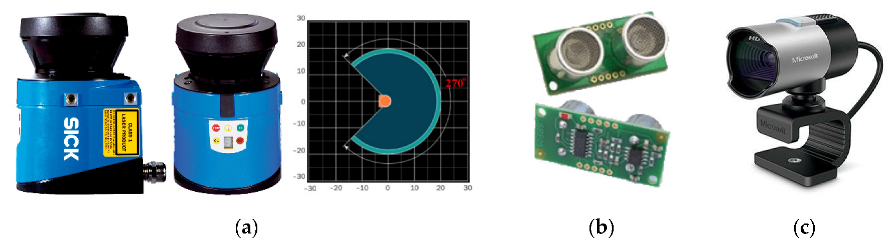
2.3. Environmental Sensors of the Robot

The SICK LMS 100 2D laser scanner is set on the fourth layer of the WMR. Its scanning angle is 270 degrees, operating range is 0.5 m to 20 m, angular resolution is 0.5 degrees, scanning frequency is 50 Hz, and operating voltage is 10.8 VDC to 30 VDC. It uses Ethernet to connect the SICK LMS 100 2D laser scanner to the notebook. Figure 2a is the appearance of the SICK LMS 100 2D laser scanner and its illustration of the scanning range [14]. The ultrasonic sensors in front of the carrier of the second layer are the Devantech SRF05 sonar sensor, detecting range is 1 cm to 4 m. SRF05 sonar sensor module is easy to connect with the ordinary control panel, such as BASICX, etc. Sonar frequency is 40 kHz, current is 4 mA, and the voltage is 5 V, as shown in Figure 2b. The robot uses a Microsoft LifeCam studio 1080P Full-HD webcam to catch the visual image. It is set on the left shoulder. Webcam is for target recognition and face recognition and is used to search the people who appear in the patrol path, as shown in Figure 2c.

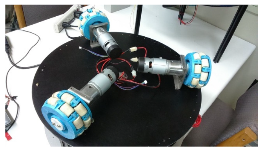
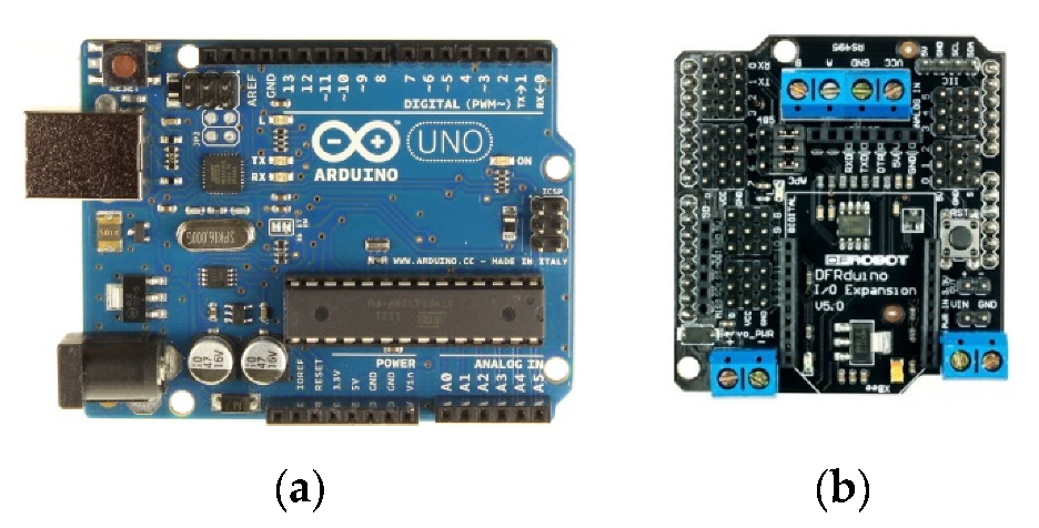
2.4. Composition of the Motion System

The omnidirectional WMR uses a three-wheel drive so that the wheels on the WMR are separated 120° to each other, as shown in Figure 3. Using three-wheel drive, the disadvantage is that the direction of WMR is difficult to control stably. However, when the WMR is set on a coordinate system [16], we can use an omnidirectional WMR kinematic model [17] to implement the motion control. In this study, microcontroller Arduino was used. Figure 4a shows the Arduino UNO, which is an ATmega328-based microcontroller board. It has 14 digital input/output pins (6 of which can be used as PWM outputs), 6 analog inputs, a 16 MHz ceramic resonator, USB connection, power jack, ICSP connector, and a reset button. The Arduino is an open-source microcontroller, and the microcontroller uses the ATMEL AVR series. It contains everything needed to support the microcontroller; simply connect it to a computer using a USB cable or boot it with an AC-to-DC adapter or battery. The DFRduino I/O expansion board is shown in Figure 4b. Arduino has a different model, hence, we used Arduino UNO and DFRduino I/O expansion board in the control scheme. With a similar Java and C development environment, it can connect other sensors and electronic components. When the direction of WMR can be controlled stably, the omni-wheels have the advantages of having no radius of gyration and being able to move in any direction compared with the ordinary differential steering.

2.5. Face Recognition

This study uses a webcam to detect the intruder who appears on the patrol path. For people detection, the important information is head, face, skin color, and so on. The image processing methods include pattern recognition, feature description, human face detection, and convolutional neural network. To start with, the webcam captures the desired color of the target in RGB color space. RGB color space uses additive color by primary color to produce many colors, but RGB color is easily influenced by the light source. Various changes will occur due to outdoor ambient light sources. Thus, the RGB image is transformed to the HSV color space, the use of HSV color space is to reduce the impact of light sources. The HSV space is similar to human vision. By color segmentation [33] we can obtain the HSV color space for pattern recognition. Then, the face image is processed by the Haar-like method [34,35,36]. The second is Adaptive Boosting (AdaBoost) learning algorithm and boosted classifiers that can have a better success rate for detecting faces [37]. The convolutional neural network (CNN) image processing is applied to face recognition. It has been proven to have a very good recognition rate. However, when CNN involves the operational nature of deep learning, it must have a huge amount of computing resources and needs a very long training time to support the final results. This study attempted to achieve generally acceptable effect verification with CNN that is as simple as possible, maintain the face recognition rate that can be generally accepted under general conditions after simplifying CNN, and use less computational resources and training time [38]. These methods are described as follows.

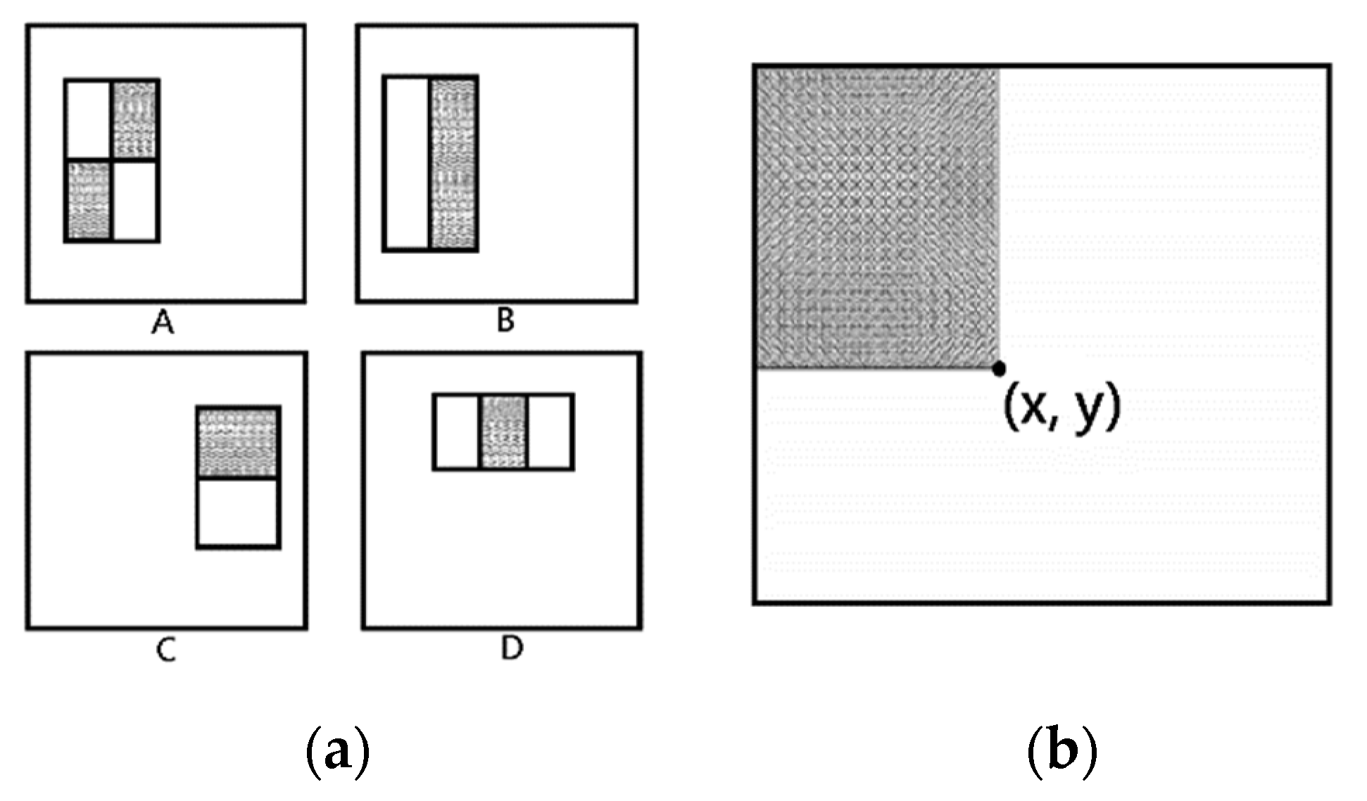
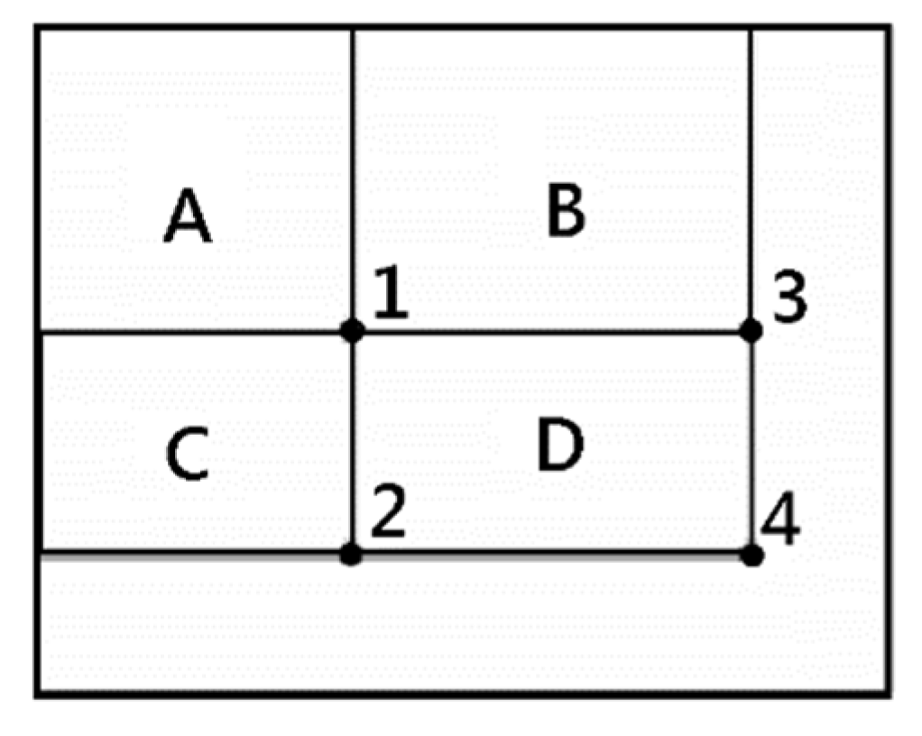
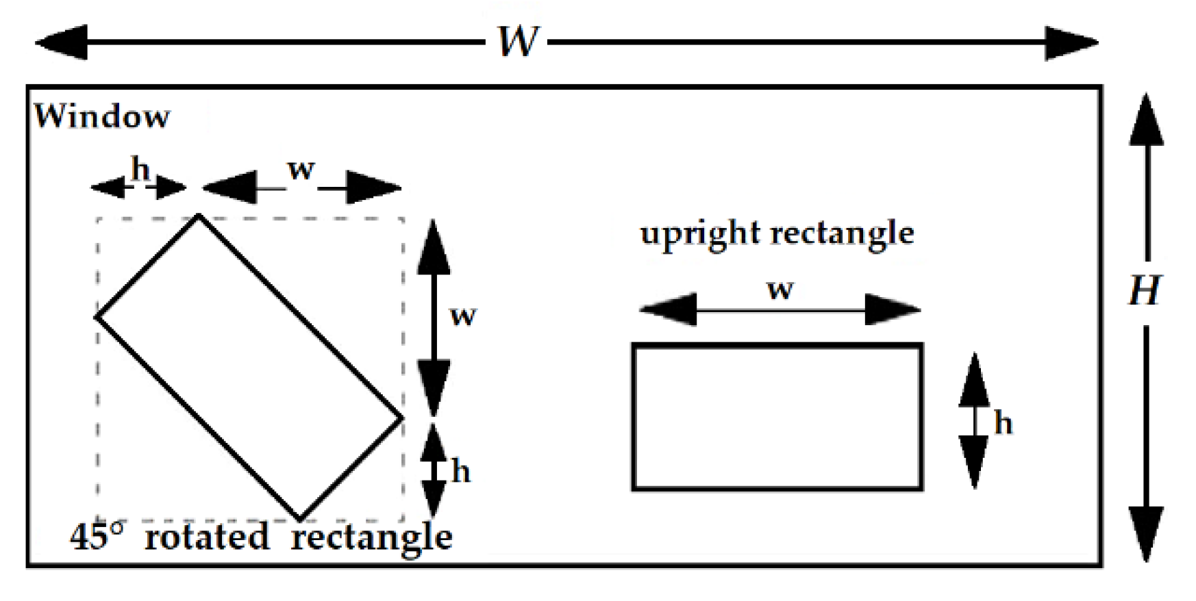
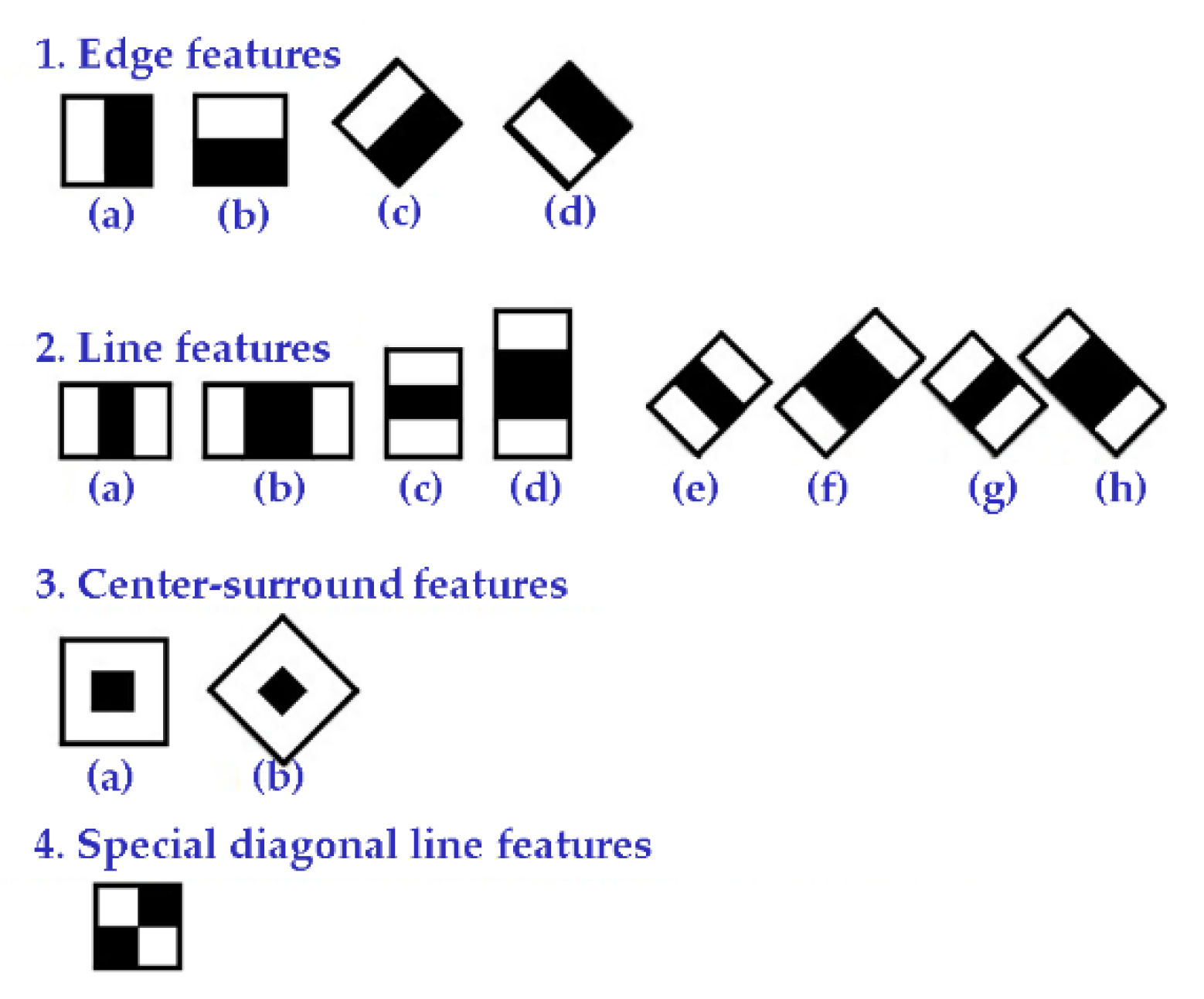
2.5.1. Integral Image

The rectangle features are shown in Figure 5a [37], and the value I(x,y) at point (x,y) in the integral image is the sum of $i\left(x^{\prime },y^{\prime }\right)$ of all the pixels $\left(x^{\prime },y^{\prime }\right)$ above and to the left of (x,y), as shown in Figure 5b [37,39,40]. Its computation is very fast at any scale or location in constant time by using the integral image, which was proposed by Frank Crow in 1984. In Equation (5), $I$ is the value of the pixel position in the integral image and $i$ is the value of the pixel position in the original image.

$$I\left(x,y\right)={\displaystyle \sum }_{x^{\prime }\le x,y^{\prime }\le y^{\prime }}x\left(x^{\prime },y^{\prime }\right)$$

(5)

The integral of the image can be computed efficiently with one pass over the image, and the value at point (x,y) is [39]:

$$I\left(x,y\right)=i\left(x,y\right)-I\left(x-1,y-1\right)+I\left(x,y-1\right)+I\left(x-1,y\right)$$

(6)

When the integral image has been computed, the rectangular sum can be computed in four array references regardless of the area size, as shown in Figure 6 [37]. That sign in Figure 6, having 1 = ($x_0$,$y_0$), 2 = ($x_1$,$y_0$), 3 = ($x_0$,$y_1$), and 4 = ($x_1$,$y_1$), the sum of i(x,y) over the rectangle spanned by 1, 2, 3 and 4 is [34]:

$${\displaystyle \sum }_{\begin{array}{c}{x}_0<x\le x_1\\ y_0<y\le y_1\end{array}}i\left(x,y\right)=I\left(4\right)+I\left(1\right)-I\left(2\right)-I\left(3\right)$$

(7)

Lienhart et al. proposed a novel set to rotate Haar-like features [35]. Their method has two assumptions, one is to assume that the basic unit for testing for the presence of an object is a window of W*H pixels, as shown in Figure 7 [35,36].

The other is to assume that they have a very fast way of computing the sum of pixels of an upright and 45° rotated rectangle inside the window. That can extend the original feature set, which is used by Viola and Jones. The calculation for 14 Haar-like features is very fast at any scale or location in a constant time, as shown in Figure 8 [35,36]. Calculation of each feature is by summing up pixels [34,40].

$$featur{e}_I={\displaystyle \sum }_{i\in I=\left\{1,\cdots ,N\right\}}{\omega }_i\ast RecSum\left(r_i\right)$$

(8)

where $w_i$ are the weights, $r_i$ are the rectangles, and N is chosen arbitrarily. Only weighted combinations of pixel sums of two rectangles are considered, that is, N = 2. The weights have opposite signs and are used to compensate for the difference in area size between the two rectangles.

At the 45° rotated rectangles, the value of the point (x,y) in the integral image is the sum of extending upwards until the boundaries of the image and all the pixels of the bottom-most corner at point (x,y), as shown in Figure 9 [36].

$$R\left(x,y\right)={\displaystyle \sum }_{y^{\prime }\le y, y^{\prime }\le y-\left|x-x^{\prime }\right|}I\left(x^{\prime },y^{\prime }\right)$$

(9)

Computation efficiently of the integral image can be performed with one pass over the image from left to right and top to bottom, as shown in Figure 10 [36].

$$R\left(x,y\right)=R\left(x-1,y-1\right)+R\left(x+1,y-1\right)-R\left(x,y-2\right)+I\left(x,y\right)+I\left(x,y-1\right)$$

(10)

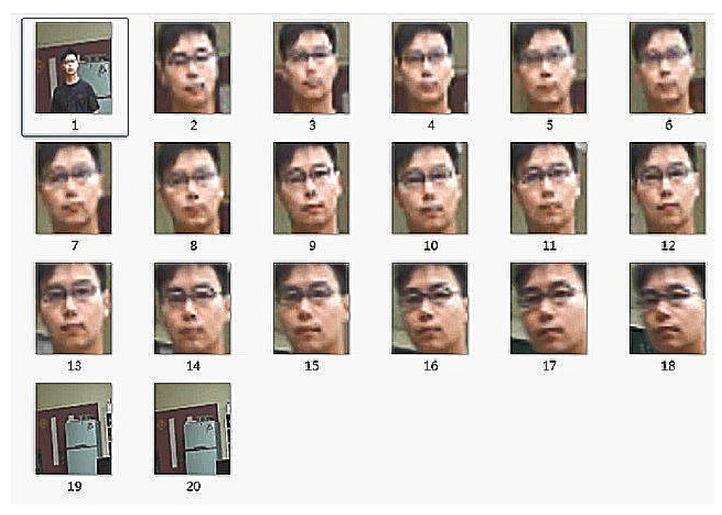
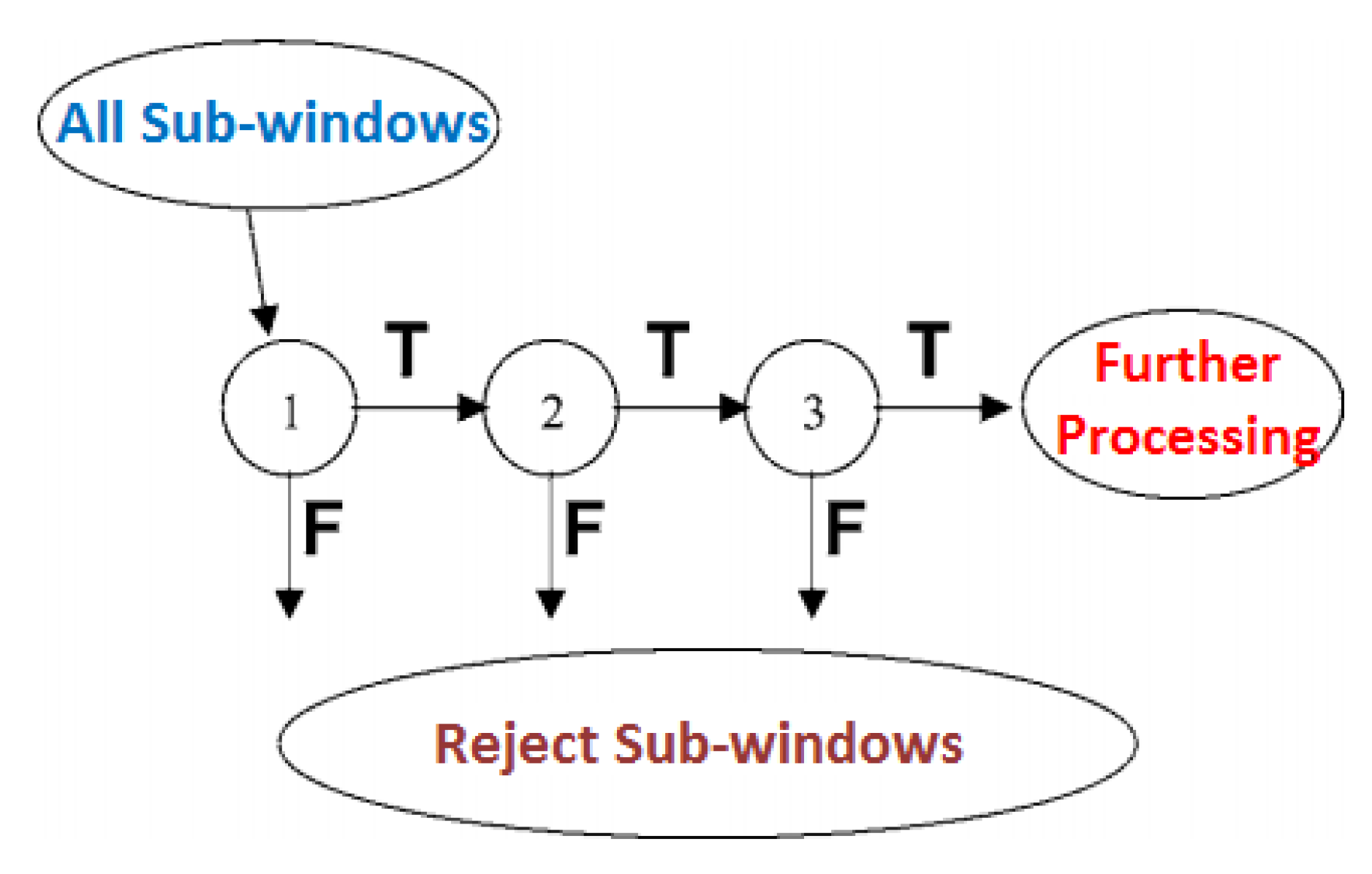
2.5.2. Adaptive Boosting and Preprocessing

In 2001, Viola and Jones utilized the detection frame that used Haar-like features of the sum of pixels in the rectangular area. The object detection framework has a good object detection rate in real-time [40]. The Haar-like method uses a rectangle frame, and its size and rotation angle can be variable. It is assumed that the first rectangle encompasses the black and white rectangle, and the second rectangle represents the black area; black areas have negative weights and white areas have positive weights (Figure 8). The feature values are different between the sum of white and dark rectangular areas of pixel values, and these different values are the basis of threshold determining whether the feature is needed or not. We use a data structure of integral graph so that calculation of rectangular features can be performed on constant time, then the adaptive boosting machine learning (AdaBoost) can classify features of selected features. The classifier function is shown in Figure 11. To ensure all face image position, skewness and size are invariant in the image, and because the distance between the eyes is nearly the same for most humans, the location of two eyes is used as a geometric normalization of face images. In the face image, the positions of the two eyes are A and B, to make a line from A to B. The line between A to B is used to maintain the level (rotating image), resulting in the direction of the face to maintain consistency, reflecting the face rotation invariance in the image plane. Figure 12 shows the relationship of scale, O is the center of the A with B. The distance is set to a fixed length (C = $\overline{\mathrm{AB}}$), reflecting the face scale invariance in the image plane, as shown in Figure 12 [41,42].

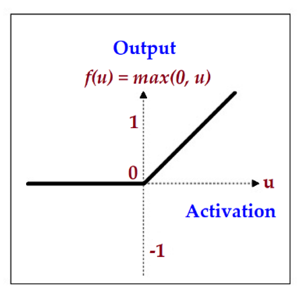
2.5.3. Convolutional Neural Network

In 2006, the article by G. Hinton and R. Salakhutdinov in Science ushered in the wave of deep learning in the academic and industrial world [43]. Their paper has two key points. The first is the multi-layer hidden artificial neural network that has excellent feature learning capabilities, and the learned features have more characterization of the data, which is conducive to visualization or classification. The other key point is deep neural network training, the difficulty of which can be effectively overcome by layer-wise pre-training. The current basic structure of the CNN consists of the input layer, convolutional layer, pooling layer, full connectivity, and output layers (classifiers). For many existing classic deep learning networks such as YOLOv4, the computing resources required from data labeling to training classification are becoming larger and larger. The process of training neural networks and adjusting hyperparameters has become very time-consuming. If we want to rely on an ordinary notebook computer to be the processor of the robot, we need to hypothesize and challenge the problem of insufficient computing power of the robot in the outdoors and minimize the demand for computing resources. The CNN model established in this experiment attempts to use only a single convolutional layer and a single pooling layer plus three full-connection layers (hidden layer, multi-layer perceptron) to reduce computing time, as shown in Figure 13. The output layer is the classifier and uses the Softmax regression.

Consider a 5 × 5 image size and a 3 × 3 convolution kernel. There are nine parameters for the convolution kernel here, which is denoted as (Theta = [theta{ij}] {3 × 3}). In this case, the convolution kernel has nine neurons, and their outputs form a 3 × 3 matrix called a feature map. The first neuron is connected to the first 3 × 3 part of the image, and the second neuron is connected to the second part (with overlap), as shown in Figure 14 [44].

Θ = [θij] 3 × 3

(11)

A matrix of (m × n) is convoluted with a matrix of (u × v) to obtain a matrix of ((m + u − 1) × (n + v − 1)).

Apply the discrete convolution operation, assuming a two-dimensional discrete function (f(m, n), g(u, v)), then their convolution is defined as f(m, n), g(u, v), and their convolution is defined as:

$$A\left(m,n\right)=f\left(m,n\right)\ast g\left(u,v\right)={{\displaystyle \sum }}_i^m{{\displaystyle \sum }}_j^{n}f\left(m-u,n-v\right)g\left(u,v\right).$$

(12)

The top of Figure 14 is the output of the first neuron, and the bottom is the output of the second neuron. The operation of each neuron is:

$$A_{\left(1+q\right)\left(1+p\right)}=act\left({{\displaystyle \sum }}_i^u{{\displaystyle \sum }}_j^v{a}_{\left(i+q\right)\left(j+p\right)}{\theta }_{ij}+b\right).$$

(13)

In Equations (11)–(13), $\Theta$ is the 9 parameters for the convolution kernel, $A\left(m, n\right)$ is the convolution output, $f\left(m,n\right)$ is the convolution input, and $g\left(u,v\right)$ is the convolution kernel, $u \left(\mathrm{and} v\right)$ is the length (and width) of the matrix of the convolution kernel, $m \left(\mathrm{and} n\right)$ is the length (and width) of the matrix of the convolution input, $act$ is the activation function, $b$ is the bias value, $i \mathrm{and} j$ are the position subscript of the matrix, $q$ is a positive integer and the range is less than or equal to (m − u), and $p$ is a positive integer and the range is less than or equal to (n − v).

The purpose of pooling is to reduce the feature map. The pool size is generally 2 × 2 [39]. Commonly used pooling methods are:

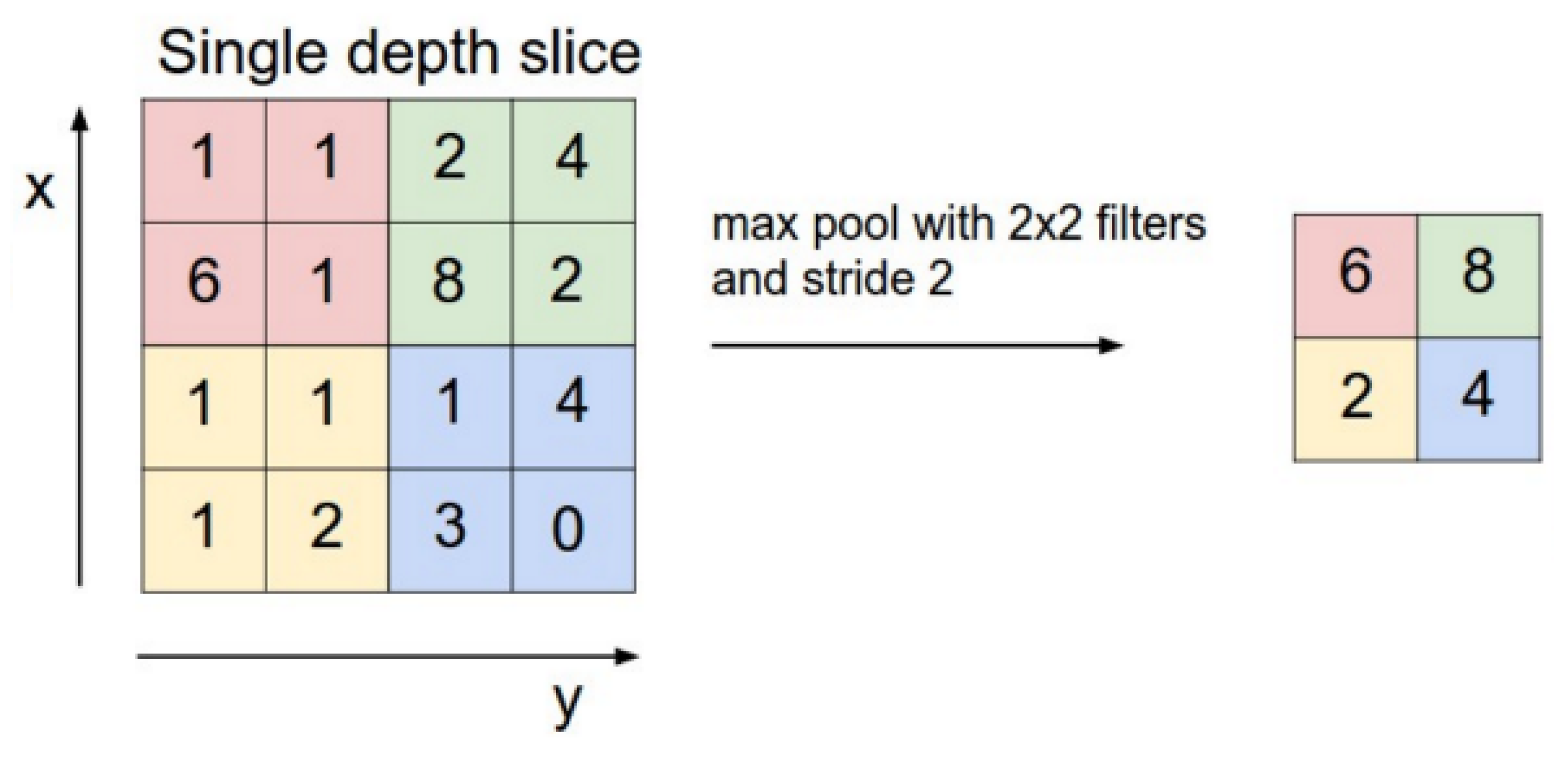
• Max Pooling, take the maximum inside of the 4 points. This pooling method is used in this study, as shown in Figure 15.
• Mean Pooling, take the average for the 4 points.
• Gaussian pooling, learn from Gaussian fuzzy methods, uncommonly used.
• It can be pooled, the training function (f) accepts 4 points as input and 1 point as output, uncommonly used.
• Since the length of the feature map is not necessarily a multiple of 2, there are also two schemes for edge processing:
• Ignore edges, save the extra edges directly.
• Keep edges, the variable length of the feature map is filled with 0 as a multiple of 2, and then pooled. This is the edge processing method used in this study.

In the fully connected network of the CNN, the layer between the input layer and the output layer is called the hidden layer. The perceptron is calculated using the following formula:

Connection weight: i is input neuron, j is output neuron:

$$W_{ji}\left(n+1\right)=W_{ji}\left(n\right)+\Delta W_{ji}\left(n\right)+\alpha \Delta W_{ji}\left(n-1\right)$$

(14)

Weight change (hidden neuron): k is the neuron in the output layer:

$$\Delta W_{ji}\left(n\right)=\eta {\dot{\phi }}_j\left(v_j\left(n\right)\right){\displaystyle \sum }_{k\in c}[{\delta }_k\left(n\right)W_{kj}\left(n\right)]y_i\left(n\right)$$

(15)

Weight change (output neuron):

$$\Delta W_{ji}\left(n\right)=\eta e_j\left(n\right){\dot{\phi }}_j\left(v_j\left(n\right)\right)y_i\left(n\right)$$

(16)

Activation (sigmoid) function:

$$\phi \left(v\right)=\frac{1}{1+\exp \left(-v\right)}$$

(17)

Local gradient (sigmoid): output layer:

$${\delta }_k=e_k{\dot{\phi }}_k\left(v_k\left(n\right)\right)=e_k{y}_k\left(n\right)\left[1-y_k\left(n\right)\right]$$

(18)

Local gradient (sigmoid): hidden layer:

$${\dot{\phi }}_j\left(v_j\left(n\right)\right)=y_k\left(n\right)\left[1-y_k\left(n\right)\right][{\displaystyle \sum }_{k\in c}{W}_{kj}\left(n\right){\delta }_k]$$

(19)

Total error:

$$\left(n\right)=\frac{1}{2}{\displaystyle \sum }_{j\in c}{e}_j^2\left(n\right), e_j\left(n\right)=d_j\left(n\right)-y_j\left(n\right)$$

(20)

Average error:

$$E_{\mathrm{av}}=\frac{1}{n}{\displaystyle \sum }_{n=1}^{\mathrm{N}}E\left(n\right)$$

(21)

In Equations (14)–(21), $W$ is the weight value of the neural network, $ji$ is the order of the weights of the neural network (the rows and columns of the weight matrix), $n$ is the iterative update timing, $\eta$ is the learning rate, $\alpha$ is the momentum, $v$ is the total input of a single neuron, $\delta$ is the local gradient, $y$ is the value of the output layer neuron, $\phi$ is the activation function, $e$ is the error value, $k$ is the serial number of the output neuron, and $d$ is the true value (ideal value).

In the traditional perceptron structure, the sigmoid function is commonly used as the activation function. To overcome the problem of vanishing gradients in multi-layer networks, Rectified Linear Unit (ReLU) can be used instead of the sigmoid function. ReLU, also known as a modified linear unit, is a commonly used activation function in artificial neural networks and usually refers to a nonlinear function represented by a ramp function and its variants [45]. The more commonly used linear rectification function has a ramp function f(x) = max(0,x), as shown in Figure 16.

In this study, the Softmax regression model was used for the final identification and classification. The Softmax regression model is an extension of the logistic regression model for multi-classification problems, wherein, the class label y can take more than two values, and Softmax regression is usually supervised [46]. In the Softmax regression, for the training set $\left\{\left(x_1,y_1\right),\dots ,\left(x_m,y_m\right)\right\}$, we have $y_{\left(i\right)}\in \left\{1,2,\dots ,k\right\}$ (note that the category index here starts with 1, not 0). For a given test input x, we can use the hypothesis function to estimate the probability value p(y=i|x) for each category j, that is, to estimate the probability of occurrence of each classification result of x. Therefore, our hypothesis function will output a k-dimensional vector (the sum of the vector elements is 1) to represent the k estimated probability values. The hypothesis function $h_{\theta }$(x) has the following form:

$$h_{\mathsf{\theta }}\left(x_{\left(i\right)}\right)=\left[\begin{array}{c}p\left(y_1=1|x_1\right)\\ p\left(y_2=2|x_2\right)\\ .\\ .\\ .\\ p\left(y_k=k|x_k\right)\end{array}\right]=\frac{1}{{{\displaystyle \sum }}_{i=1}^k{e}^{\theta x_{\left(i\right)}}}\left[\begin{array}{c}{e}^{{\theta }_1\left(x_1\right)}\\ e^{{\theta }_2\left(x_2\right)}\\ .\\ .\\ .\\ e^{{\theta }_k\left(x_k\right)}\end{array}\right]$$

(22)

When implementing Softmax regression, it would be convenient to represent θ with a matrix of k ∗ (n + 1), which is a list of ${\theta }_1$, ${\theta }_2$, …,${\theta }_{\mathrm{k}}$, as shown below:

$$\theta =\left[\begin{array}{c}{\theta }_1\\ {\theta }_2\\ .\\ .\\ .\\ {\theta }_k\end{array}\right]$$

(23)

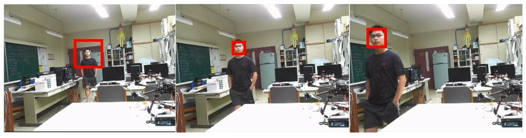
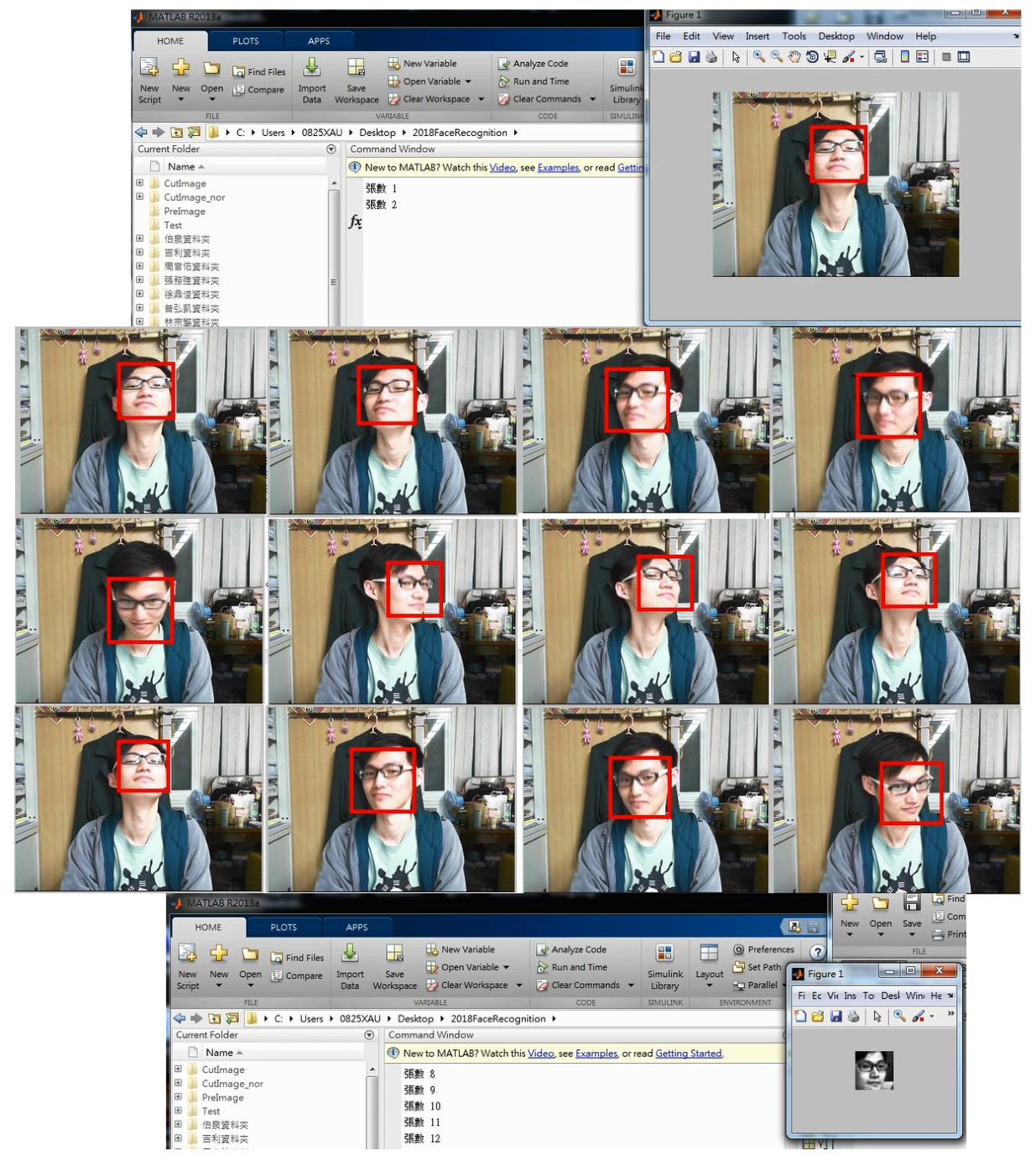
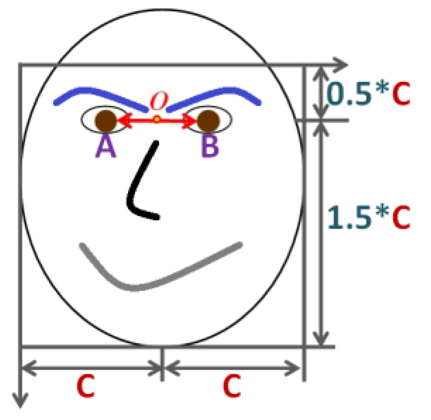
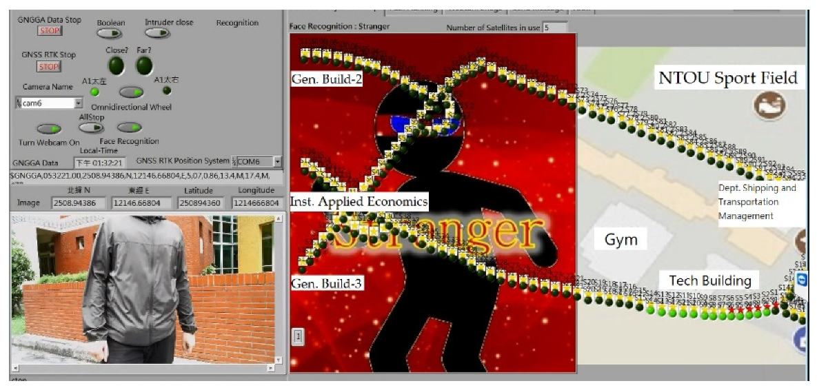
2.5.4. Real-Time Face Detection in Dynamic Background

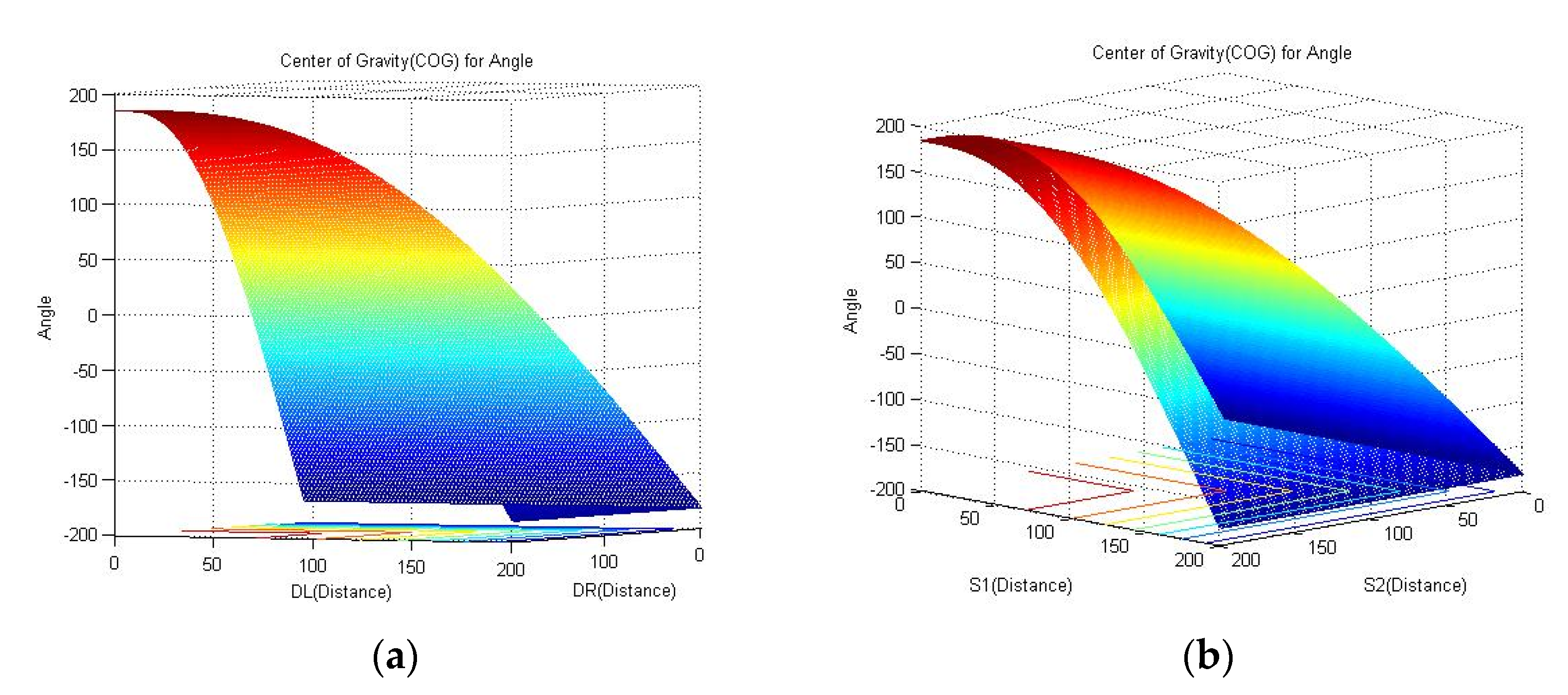
The traditional face recognition research mostly focuses on a single static image. However, the image is easily affected by the capturing environment in a dynamic background, such as local light and shadow effects and face rotation angle problems, leading to reduced recognition performance. In real-time face recognition, we try to create a better face detection rate than other methods and to overcome the decline in recognition rate, due to the lightweight of the convolutional neural network and the dynamic recognition of human faces. Our solution is to identify the same person multiple times in the streaming video of the webcam. Then multiple identification results are combined to confirm the identification of the images, as shown in Appendix A.

2.6. Fuzzy Control

The WMR must have the ability to avoid obstacles and is not influenced by obstacles in the patrol process to successfully conduct outdoor patrols. Often, vehicles parked on the road are the obstacles that are most encountered in outdoor patrols. We used a laser rangefinder to detect the obstacle which is on the patrol path and the fuzzy controller to enable the WMR to avoid obstacles. The SICK LMS100 laser rangefinder is settled on the WMR. The angle 20° of the laser rangefinder on the WMR is marked as DL. The angle 90°of the laser rangefinder on the WMR is marked as DF. The angle 160° of the laser rangefinder on the WMR is marked as DR. Input variables dl, df, and dr are presented by three linguistic labels: “near”, “medium”, and “far”. The robot uses an ultrasonic sensor and laser sensor to detect the distance of surroundings. There are three inputs of the proposed fuzzy controllers for angle control, which are detected distances from different angles. The three inputs of the fuzzy controller in angles are 20°, 90°, and 160°. For input variables 20° (dl), 90° (df), and 160° (dr), their fuzzy sets are “near”, “medium”, and “far” (the distance detection range is 0 to 200 cm). The output of the fuzzy controller is the turning angle. Fuzzy sets of the output variable for turning angle are five linguistic labels, including “VLL (turn left very large)”, “VL (turn left)”, “S (go forward)”, “VR (turn right)”, and “VRR (turn right very large)”. We established a new kind of ideal fuzzy control model through the cross combination of Gaussian functions. This fuzzy control model is shown in Figure 17. The fuzzy truth table shows all the rules used to control the steering angle, as shown in Appendix C.

In addition, we also tried five inputs, three membership functions, and 243 fuzzy rules. Compared with 243 fuzzy rules, 27 fuzzy rules were found to be sufficient to complete a patrol and avoid obstacles.

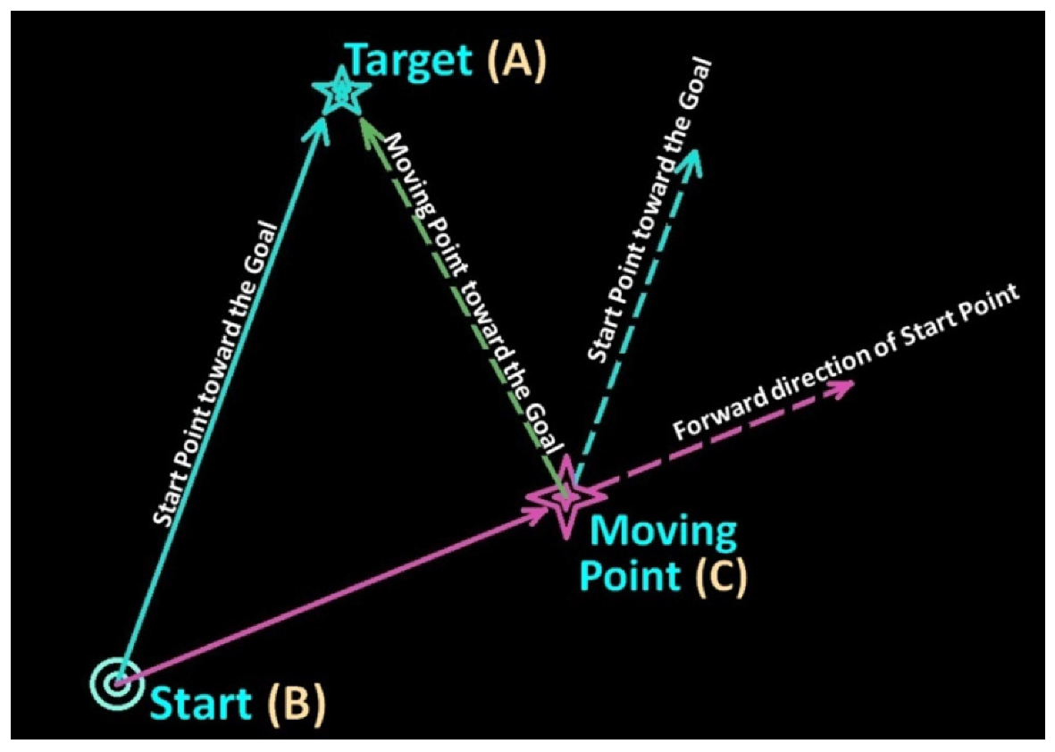
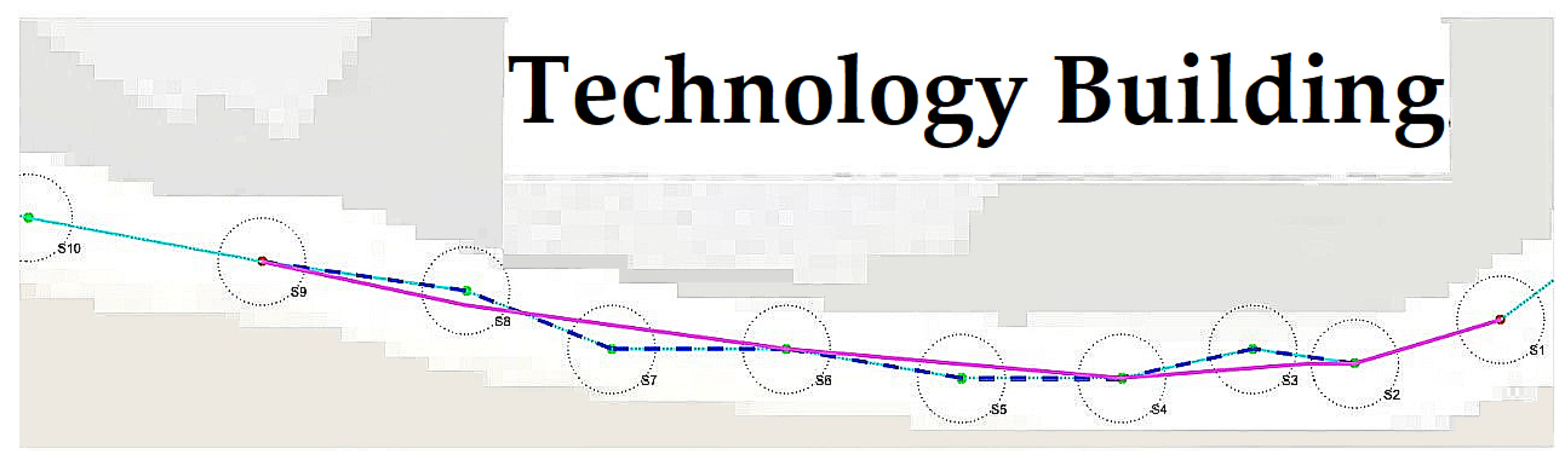
2.7. The Path Planning

When the robot performs outdoor patrol, the computing time of the road path planning should be minimized. Dijkstra algorithm can be used to calculate and shorten the operation time of the path planning, and the ant algorithm can optimize the path in path planning. Therefore, our path planning uses a combination of the Dijkstra algorithm and ant algorithm to achieve the preset goals, that too are calculated in a short time, and that the calculated path is the better or the shortest. Dijkstra algorithm is used to plan the shortest path between nodes, and since only the nodes are connected to the node that forms the shortest path, computational time can be reduced. This path planning is the shortest straight line between nodes, while the calculated path between the starting point and the ending point is often no longer the shortest. Then, the use of an ant algorithm can make up for this shortcoming. The ant algorithm is used to search for the best path to the target node. Path planning results of the Dijkstra and ant algorithms are shown in Figure 18 and Figure 19. Here, we first used the Dijkstra algorithm to plan the short path from node to node, as shown in Figure 18. Then, the ant algorithm was used to search for a shorter path along the previous calculated path from number 1 node to number 9 node, as shown in Figure 19.

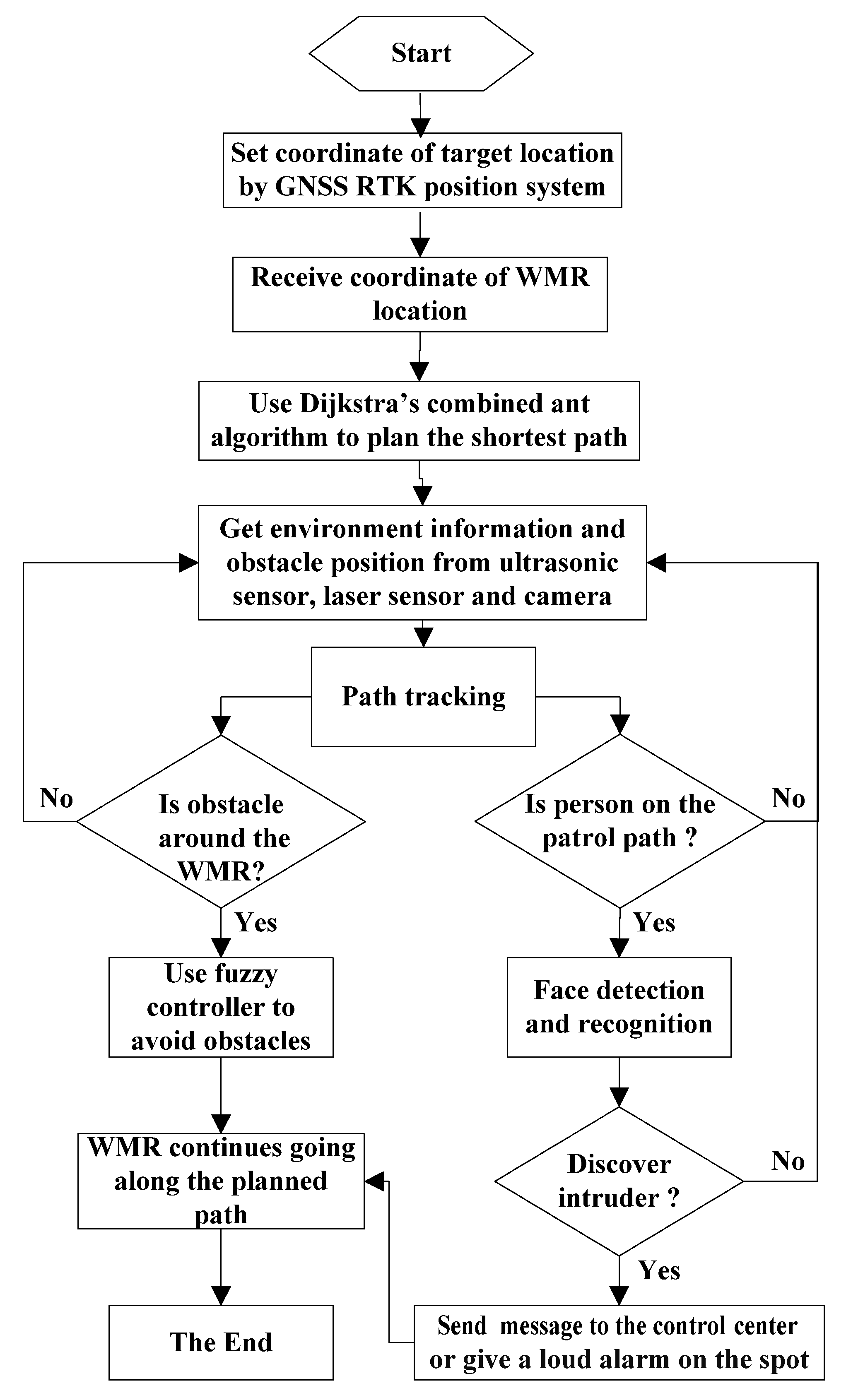
2.8. The Control Scheme

The control scheme consists of two sections. The first part is path tracking control for omnidirectional WMR navigation, which has path planning using the Dijkstra algorithm with ant algorithm and directional guidance using the GNSS RTK position system. Path correction uses Three-point positioning to determine the direction, as shown in Appendix D. The obstacles and distance are captured by laser sensor during movement. The second part is for face detection and recognition. When the robot patrols and finds an intruder, it will send the image of the intruder and the location information to the control center and give a loud alarm at the site. These two parts are integrated to control the WMR for performing outdoor patrol tasks. Figure 20 shows the flowchart of the control sequence in this study. To start with, the coordinate location of the goal of the WMR is set. After that, the GNSS RTK positioning system receiver receives the coordinate location of the WMR and then uses the Dijkstra algorithm with ant algorithm to plan the shortest path. Next, we use the ultrasonic sensor, laser sensor, and webcam to search the surrounding environment while WMR is moving. This provides environmental information and the WMR will determine the obstacles or the people that appear on the patrol path. If obstacles appear on the patrol path, then the fuzzy controller is used to avoid them until the WMR finishes the patrol. If people appear on the patrol path, the WMR will capture the images of the people from the webcam and use image detection and face recognition. If someone appears in the patrol path and the detection discovers that the person is an intruder, the WMR will save the photos of the intruder as well as the location information and send them to the control center by Wi-Fi and ask for help and give a loud alarm at the site. The experimental condition at the National Taiwan Ocean University is shown in Figure 21.

3. Results

To show the effectiveness of the control scheme proposed in this study, experiments were performed in an outdoor environment. In the experiment, we used the LabVIEW software to write a human–machine interface and used the MATLAB R2013a software to code image process, face recognition, path planning, and fuzzy controller. The SICK LMS100 laser rangefinder uses an Ethernet cable, the webcams and GNSS RTK positioning system use a USB cable to connect with a notebook, and then the notebook transmits the signals to the robot. Experiments were conducted on the campus of the National Taiwan Ocean University. The data and figures of face detection are shown in Appendix B.

In the beginning, the robot received the satellite data by the GNSS RTK positioning system and a patrol destination on the campus map was given, then the WMR started to patrol. Patrol path was obtained by the Dijkstra algorithm and ant algorithm, as shown in Figure 22. Figure 23 shows that the robot encountered a moving object, and the object was identified as a known person, as shown in Figure 24 and Figure 25. The robot kept moving along the desired path and encountered another person, as shown in Figure 26 and Figure 27. Figure 28 shows that the intruder was identified as a stranger. The robot then stopped moving and activated the alarm system, as shown in Figure 29, Figure 30 and Figure 31. Figure 32 shows a staff of the control center who went to turn off the alarm. The intruder’s image and location were sent to the control center, as shown in Figure 33 and Figure 34. Outdoor patrols at night are shown in Figure 35 and Figure 36. The left side of Figure 35 was taken by an outdoor camera, while the picture on the upper right side was taken from the notebook computer on the robot, and the picture on the bottom right side was taken by an indoor camera (in control center).

4. Discussion

During the development and realization of the robot, we once faced a difficult situation when the robot was walking on grass and gravel roads. When walking on certain rugged roads, the entire robot shakes like an inverted pendulum due to the vibration caused by the omnidirectional wheel. When the shaking period meets a certain frequency, the robot may even fall. Although this problem is caused by the robot’s center of gravity and omnidirectional wheel specifications, as a solution, we reduced the robot’s moving speed and increased the number of batteries at the bottom of the robot to adjust the center of gravity. Consequently, the endurance of the robot increased; it could patrol for 1 to 2 hours each time and reduce the demand for rapid response time for obstacle avoidance. In the area of image processing and face recognition, we used the repeated recognition method to improve the accuracy, with the advantage that even a single recognition error cannot affect the overall recognition rate, so it can overcome the impact of the poor classification ability due to the light effect and save several training resources and time spent on the entire neural network. However, the disadvantage is the increase in the time spent on face recognition. We made a few adjustments to sample pictures of the known targets in dynamic to perform classification. The image calculation could be completed in 1 second. For the result of a robot replacing a human in patrol, we send back the message of the detected person to the remote-control center. This has three advantages. First, when the robot’s recognition result is a stranger or an intruder, the personnel of the control center can reconfirm and decide whether a security guard is needed to the place of the incident. The second is data transmission and mailing through the 4G network. The coordinates and images of people can be known in detail. Naturally, it can also be set to automatically send messages to community guards or police stations when an incident occurs. Finally, during the patrol process, the image captured by the robot camera is synchronized back to the control center. If the personnel of the control center see an abnormality on the screen that the robot has not found, they can react immediately. Indeed, if the control center can have sufficient data transmission and computing performance, it is entirely possible to set up a robot formation to cover the patrolling and supporting tasks in the desired area.

5. Conclusions

In this study, an intelligent control scheme was proposed which can control a robot to perform outdoor patrol tasks day and night, and provide environmental security services. We could successfully integrate the satellite positioning system, path planning, path navigation, laser rangefinder, webcams, fuzzy controller, omnidirectional wheels robot, robotic arm, and convolutional neural network image processing to a wheeled mobile robot. Path guidance used outdoor navigation and positioning system, to obtain location information from the GNSS RTK positioning system. The Dijkstra algorithm and the ant algorithm for shortest path planning were used to compute the desired path. The GNSS RTK positioning system was used to provide the current position of WMR and this system can receive GPS + BDS observation data. As the number of useful satellites has become more than twice the number of a single satellite system, the positioning accuracy has therefore improved significantly. The laser rangefinder and the fuzzy controller were used to detect the surroundings and avoid obstacles in real-time. In image processing, a normal image was in RGB color space, and the produced color was not so intuitive and susceptible to light interference. An object with the light intensity changes will have a large difference in the same image and is difficult to distinguish for identification. Thus, we used HSV color space to solve the problem of light interference, as it can counter the influence of the light source more effectively. It also has a better identification effect for the light source changes during a night patrol. In face recognition, we used a simplified convolutional neural network for classification, and the experimental results prove the feasibility of this method. Two webcams and image processing were used to acquire and recognize the images of the patrol process, detect the intruder who appears on the patrol path, and capture the photo of the intruder. Although the robot sometimes recognizes people as strangers due to light problems during nighttime, as long as the staff of the central control center check the photo of the intruder sent by the robot, they can confirm whether a stranger has invaded. Experiment results show that the WMR can complete outdoor patrol tasks during the day or night, successfully detect the intruder in the patrol process, send the intruder’s photo to the control center, and therefore validate the effectiveness of the control scheme that was proposed in this study. The outdoor security robot designed in this study has the advantages of replacing human patrol and reducing manpower requirements, as well as succeeded in cheaper assembly costs of the robot.

References

1. Juang, J.G.; Chen, H.S.; Lin, C.C. Intelligent path tracking and motion control for wheeled mobile robot. GESTS Int. Trans. Comput. Sci. Eng. 2010, 61, 57–68. [Google Scholar]
2. Ohya, A.; Kosaka, A.; Kak, A. Vision-based navigation by a mobile robot with obstacle avoidance using single-camera vision and ultrasonic sensing. IEEE Trans. Robot. Autom. 1998, 14, 969–978. [Google Scholar] [CrossRef]
3. Juang, J.-G.; Tsai, Y.-J.; Fan, Y.-W. Visual recognition and its application to robot arm control. Appl. Sci. 2015, 5, 851–880. [Google Scholar] [CrossRef]
4. Coelho, J.; Ribeiro, F.; Dias, B.; Lopes, G.; Flores, P. Trends in the Control of Hexapod Robots: A survey. Robotics 2021, 10, 100. [Google Scholar] [CrossRef]
5. Azizi, M.R.; Rastegarpanah, A.; Stolkin, R. Motion planning and control of an omnidirectional mobile robot in dynamic environments. Robotics 2021, 10, 48. [Google Scholar] [CrossRef]
6. Qian, J.; Zi, B.; Wang, D.; Ma, Y.; Zhang, D. The design and development of an omni-directional mobile robot oriented to an intelligent manufacturing system. Sensors 2017, 17, 2073. [Google Scholar] [CrossRef] [PubMed] [Green Version]
7. Kanjanawanishkul, K. Omnidirectional wheeled mobile robots: Wheel types and practical applications. Int. J. Adv. Mechatron. Syst. 2015, 6, 289–302. [Google Scholar] [CrossRef]
8. Juang, J.G.; Hsu, K.J.; Lin, C.M. A wheeled mobile robot path-tracking system based on image processing and adaptive CMAC. J. Mar. Sci. Technol. 2014, 22, 331–340. [Google Scholar]
9. Pastore, T.H.; Everett, H.R.; Bonner, K. Mobile Robots for Outdoor Security Applications. 1999. Available online: https://www.semanticscholar.org (accessed on 21 March 2018).
10. Ohno, K.; Tsubouchi, T.; Shigematsu, B.; Yuta, S. Differential GPS and odometry-based outdoor navigation of a mobile robot. Adv. Robot. 2004, 18, 611–635. [Google Scholar] [CrossRef]
11. Maram, S.S.; Vishnoi, T.; Pandey, S. Neural Network and ROS based threat detection and patrolling assistance. In Proceedings of the International Conference on Advanced Computational and Communication Paradigms, Gangtok, India, 25–28 February 2019. [Google Scholar]
12. Fava, A.D.; Satler, M.; Tripicchio, P. Visual navigation of mobile robots for autonomous patrolling of indoor and outdoor areas. In Proceedings of the Mediterranean Conference on Control and Automation, Torremolinos, Spain, 16 July 2015. [Google Scholar]
13. Shin, Y.; Jung, C.; Chung, W. Drivable road region detection using a single laser range finder for outdoor patrol robots. In Proceedings of the IEEE Intelligent Vehicles Symposium, La Jolla, CA, USA, 21–24 June 2010. [Google Scholar]
14. Kartikey, A.D.; Srivastava, U.; Srivastava, V.; Rajesh, S. Nonholonomic shortest robot path planning in a dynamic environment using polygonal obstacles. In Proceedings of the IEEE International Conference on Industrial Technology, Via del Mar, Chile, 14–17 March 2010. [Google Scholar]
15. Lin, R.; Li, M.; Sun, L. Real-time objects recognition and obstacles avoidance for mobile robot. In Proceedings of the IEEE International Conference on Robotics and Biomimetics, Shenzhen, China, 12–14 December 2013. [Google Scholar]
16. Sun, T.; Wang, Y.; Yang, J.; Hu, X. Convolution neural networks with two pathways for image style recognition. IEEE Trans. Image Process. 2017, 26, 4102–4113. [Google Scholar] [CrossRef] [PubMed]
17. Huang, G.S.; Tung, C.K.; Lin, H.C.; Hsiao, S.H. Inverse kinematics analysis trajectory planning for a robot arm. In Proceedings of the 8th Asian Control Conference, Kaohsiung, Taiwan, 15–18 May 2011. [Google Scholar]
18. Lian, S.H. Fuzzy logic control of an obstacle avoidance robot. In Proceedings of the 5th IEEE International Conference on Fuzzy Systems, New Orleans, LA, USA, 11 September 1996. [Google Scholar]
19. Chung, J.H.; Yi, B.J.; Kim, W.K.; Lee, H. The dynamic modeling and analysis for an omnidirectional mobile robot with three caster wheels. In Proceedings of the 2003 IEEE International Conference on Robotics & Automation, Taipei, Taiwan, 14–19 September 2003. [Google Scholar]
20. Aman, M.S.; Mahmud, M.A.; Jiang, H.; Abdelgawad, A.; Yelamarthi, K. A sensor fusion methodology for obstacle avoidance robot. In Proceedings of the IEEE International Conference on Electro Information Technology, Grand Forks, ND, USA, 19–21 May 2016. [Google Scholar]
21. Fukai, H.; Mitsukura, Y.; Xu, G. The calibration between range sensor and mobile robot, and construction of an obstacle avoidance robot. In Proceedings of the 21st IEEE International Symposium on Robot and Human Interactive Communication, Paris, France, 9–13 September 2012. [Google Scholar]
22. Liu, Y.; Wu, X.; Zhu, J.; Lew, J. Omni-directional mobile robot controller design by trajectory linearization. In Proceedings of the American Control Conference, Denver, CO, USA, 4–6 June 2003. [Google Scholar]
23. Lin, K.H.; Lee, H.S.; Chen, W.-T. Implementation of obstacle avoidance and zigbee control functions for omni directional mobile robot. In Proceedings of the 2008 IEEE International Conference on Advanced Robotics and Its Social Impacts, Taipei, Taiwan, 23–25 August 2008. [Google Scholar]
24. Zhang, L.; Min, H.; Wei, H.; Huang, H. Global path planning for mobile robot based on a* algorithm and genetic algorithm. In Proceedings of the IEEE International Conference on Robotics and Biomimetics, Guangzhou, China, 11–14 December 2012. [Google Scholar]
25. Fadzli, S.A.; Abdulkadir, S.I.; Makhtar, M.; Jamal, A.A. Robotic indoor path planning using dijkstra’s algorithm with multi-layer dictionaries. In Proceedings of the 2nd International Conference on Information Science and Security, Seoul, Korea, 14–16 December 2015. [Google Scholar]
26. Kho, T.; Salih, M.H.; Woo, Y.S.; Ng, Z.; Min, J.J.; Yee, F. Enhance implementation of embedded robot auto-navigation system using FPGA for better performance. In Proceedings of the 3rd International Conference on Electronic Design, Phuket, Thailand, 11–12 August 2016. [Google Scholar]
27. North, E.; Georgy, J.; Tarbouchi, M.; Iqbal, U.; Noureldin, A. Enhanced mobile robot outdoor localization using INS/GPS integration. In Proceedings of the International Conference on Computer Engineering & Systems, Caitro, Egypt, 14–16 December 2009. [Google Scholar]
28. Mahendran, A.; Vedaldi, A. Understanding deep image representations by inverting them. In Proceedings of the IEEE conference on Computer Vision and Pattern Recognition (CVPR), Boston, MA, USA, 7–12 June 2015. [Google Scholar]
29. Shuyun, H.; Shoufeng, T.; Bin, S. Robot path planning based on improved ant colony optimization. In Proceedings of the International Conference on Robots & Intelligent System (ICRIS), Changsha, China, 26–27 May 2018. [Google Scholar]
30. Xiu, C.; Lai, T.; Chai, Z. Design of automatic handling robot control system. In Proceedings of the Chinese Control and Decision Conference (CCDC), Shenyang, China, 9–11 June 2018. [Google Scholar]
31. Parada-Salado, J.G.; Ortega-Garcia, L.E.; Ayala-Ramirez, L.F.; Perez-Pinal, F.J.; Herrera-Ramirez, C.A.; Padilla-Medina, J.A. A low-cost land wheeled autonomous mini-robot for in-door surveillance. IEEE Lat. Am. Trans. 2018, 16, 1298. [Google Scholar] [CrossRef]
32. Isakhani, H.; Aouf, N.; Kechagias-Stamatis, O.; Whidborne, J.F. A furcated visual collision avoidance system for an autonomous micro robot. IEEE Trans. Cogn. Dev. Syst. 2018, 12, 1. [Google Scholar] [CrossRef]
33. Luo, L.; Li, X. A method to search for color segmentation threshold in traffic sign detection. In Proceedings of the International Conference on Image and Graphics, Xi’an, China, 20–23 September 2009. [Google Scholar]
34. Shih, C.-H.; Juang, J.-G. Moving object tracking and its application to indoor dual-robot patrol. Appl. Sci. 2016, 6, 349. [Google Scholar] [CrossRef] [Green Version]
35. Lienhart, R.; Maydt, J. An extended set of haar-like features for rapid object detection. In Proceedings of the International Conference on Image Processing, Rochester, NY, USA, 22–25 September 2002. [Google Scholar]
36. Lienhart, R.; Kuranov, A.; Pisarevsky, V. Empirical analysis of detection cascades of boosted classifiers for rapid object detection. In Proceedings of the 25th DAGM Symposium on Pattern Recognition, Magdeburg, Germany, 10–12 September 2003. [Google Scholar]
37. Viola, P.; Jones, M. Robust real-time face detection. Int. J. Comput. Vis. 2004, 57, 137–154. [Google Scholar] [CrossRef]
38. Qi, X.; Liu, C.; Schuckers, S. CNN based key frame extraction for face in video recognition. In Proceedings of the IEEE 4th International Conference on Identity, Security, and Behavior Analysis, Potsdam, NY, USA, 11–12 January 2018. [Google Scholar]
39. Wikipedia, Summed Area Table. Available online: https://en.wikipedia.org/wiki/Summed_area_table (accessed on 12 December 2017).
40. Viola, P.; Jones, M. Rapid object detection using a boosted cascade of simple features. In Proceedings of the IEEE Computer Society Conference on Computer Vision and Pattern Recognition, Kauai, HI, USA, 8–14 December 2001. [Google Scholar]
41. Kruppa, H.; Castrillon-Santana, M.; Schiele, B. Fast and robust face finding via local context. In Proceedings of the Joint IEEE International Workshop on Visual Surveillance and Performance Evaluation of Tracking and Surveillance, Beijing, China, 12–13 October 2003. [Google Scholar]
42. Chen, C.-L.; Wang, P.-B.; Juang, J.-G. Application of real-time positioning system with visual and range sensors to security robot. Sens. Mater. 2019, 31, 543. [Google Scholar] [CrossRef] [PubMed] [Green Version]
43. Hinton, G.E.; Salakhutdinov, R.R. Reducing the dimensionality of data with neural networks. Science 2006, 313, 504. [Google Scholar] [CrossRef] [PubMed] [Green Version]
44. Saito, K. Deep Learning; Gotop Information Inc.: Taipei, Taiwan, 2017. [Google Scholar]
45. Available online: https://zh.wikipedia.org/wiki/%E7%BA%BF%E6%80%A7%E6%95%B4%E6%B5%81%E5%87%BD%E6%95%B0 (accessed on 18 August 2021).
46. Available online: http://ufldl.stanford.edu/wiki/index.php/Softmax%E5%9B%9E%E5%BD%92 (accessed on 18 August 2021).
Figure 1. (a) The omnidirectional WMR with webcam, laser sensor, ultrasonic sensors, GNSS RTK positioning system, StarGazer positioning system, and notebook; (b) the GNSS antenna and the GNSS receiver [8].
Applsci 11 08857 g001
Figure 2. (a) The appearance and the scanning range of the SICK LMS 100 2D laser scanner [14]; (b) Microsoft LifeCam studio webcam [15]; (c) Devantech SRF05 sonar sensor module.
Applsci 11 08857 g002
Figure 3. The three wheels of an omnidirectional WMR.
Applsci 11 08857 g003
Figure 4. (a) Arduino UNO; (b) DFRduino I/O expansion board.
Applsci 11 08857 g004
Figure 5. (a) Each rectangle feature is a single value obtained by subtracting the sum of the pixels which lie within the white rectangles from the sum of pixels in the gray rectangles; (b) the value I(x,y) at point ( x ,   y ) in the integral image is the sum of all the pixels above and to the left of ( x ,   y ) .
Applsci 11 08857 g005
Figure 6. The sum of the pixels within rectangle D can be computed with four array references.
Applsci 11 08857 g006
Figure 7. The examples of upright and 45° rotated rectangles.
Applsci 11 08857 g007
Figure 8. The extended feature sets, wherein, the black and white areas correspond to positive and negative weights, respectively.
Applsci 11 08857 g008
Figure 9. The value at point ( x ,   y ) in the integral image is the sum of all the pixels of the bottom-most corner at point ( x ,   y ) and extending upwards until the boundaries of the image.
Applsci 11 08857 g009
Figure 10. Calculation scheme for the integral image.
Applsci 11 08857 g010
Figure 11. The Cascaded classifier.
Applsci 11 08857 g011
Figure 12. Image clipping ratio diagram.
Applsci 11 08857 g012
Figure 13. The structure of CNN.
Applsci 11 08857 g013
Figure 14. The convolutional process.
Applsci 11 08857 g014
Figure 15. The pooling process.
Applsci 11 08857 g015
Figure 16. The Rectified Linear Unit (ReLU) function.
Applsci 11 08857 g016
Figure 17. (a) Two input variables and one output variable of turning angles-1; (b) turning angles-2.
Applsci 11 08857 g017
Figure 18. Path planning by Dijkstra algorithm.
Applsci 11 08857 g018
Figure 19. Path planning by Dijkstra algorithm combined with ant algorithm.
Applsci 11 08857 g019
Figure 20. Flowchart of the control sequence.
Applsci 11 08857 g020
Figure 21. The testing field in National Taiwan Ocean University (WGS84: N25.14993733502751, E121.77837084706557).
Applsci 11 08857 g021
Figure 22. The robot started patrolling according to the path planning on the map.
Applsci 11 08857 g022
Figure 23. The robot encountered a person appearing in front of it.
Applsci 11 08857 g023
Figure 24. The robot identified the person appearing in front of it.
Applsci 11 08857 g024
Figure 25. The robot displayed the identified person on the screen.
Applsci 11 08857 g025
Figure 26. The robot patrolled towards the destination.
Applsci 11 08857 g026
Figure 27. Someone appeared on the pathway.
Applsci 11 08857 g027
Figure 28. The robot identified the intruder as a stranger.
Applsci 11 08857 g028
Figure 29. The robot’s arm started to activate the alarm.
Applsci 11 08857 g029
Figure 30. The robot raised hands and gave a loud alarm at the site.
Applsci 11 08857 g030
Figure 31. The robot activated the alarm and stopped moving.
Applsci 11 08857 g031
Figure 32. Personnel from the control center went to turn off the alarm.
Applsci 11 08857 g032
Figure 33. The control center received face pictures of the stranger.
Applsci 11 08857 g033
Figure 34. The location of the stranger being indicated on the map in real-time (WGS84: N25.14993733502751, E121.77837084706557).
Applsci 11 08857 g034
Figure 35. The robot patrolled in the nighttime and encountered a stranger passing by.
Applsci 11 08857 g035
Figure 36. The robot patrolled in the night and identified the person passing by as a stranger.
Applsci 11 08857 g036
Publisher’s Note: MDPI stays neutral with regard to jurisdictional claims in published maps and institutional affiliations.