Empirical Study of Constraint-Handling Techniques in the Optimal Synthesis of Mechanisms for Rehabilitation

Abstract

Currently, rehabilitation systems with closed kinematic chain mechanisms are low-cost alternatives for treatment and health care. In designing these systems, the dimensional synthesis is commonly stated as a constrained optimization problem to achieve repetitive rehabilitation movements, and metaheuristic algorithms for constrained problems are promising methods for searching solutions in the complex search space. The Constraint Handling Techniques (CHTs) in metaheuristic algorithms have different capacities to explore and exploit the search space. However, the study of the relationship in the CHT performance of the mechanism dimensional synthesis for rehabilitation systems has not been addressed, resulting in an important gap in the literature of such problems. In this paper, we present a comparative empirical study to investigate the influence of four CHTs (penalty function, feasibility rules, stochastic-ranking, and $ϵ$-constraint) on the performance of ten representative algorithms that have been reported in the literature for solving mechanism synthesis for rehabilitation (four-bar linkage, eight-bar linkage, and cam-linkage mechanisms). The study involves analysis of the overall performance, six performance metrics, and evaluation of the obtained mechanism. This identified that feasibility rules usually led to efficient optimization for most analyzed algorithms and presented more consistency of the obtained results in these kinds of problems.

1. Introduction

The increasing number of people with motor deficiencies has been a crucial factor in developing rehabilitation devices. Motor injuries frequently occur in the upper and lower extremities due to degenerative diseases, neuronal disorders, sports injuries, traffic, and work accidents. Presently, rehabilitation devices for upper and lower limbs have been developed [1,2]. Stationary rehabilitation devices are used more frequently in the rehabilitation of the patient. However, these devices are generally expensive because the control of several degrees of freedom is required to generate a rehabilitation routine. Rehabilitation systems based on closed-chain mechanisms are a low-cost alternative for health care [3]. These systems can provide a pre-established rehabilitation routine that controls a degree of freedom. Therefore, these devices can be considered for rehabilitation at home.

In the design of closed-chain mechanisms, a synthesis process of the mechanism is carried out [4]. In this process, the length of links is determined to achieve the desired movements for rehabilitation. The graphic, analytic, and optimal methods [5] are the used techniques for the synthesis of closed-chain mechanisms. Graphic synthesis of mechanisms is performed by a visual representation of the mechanism, where Euclidean geometry concepts are used to obtain the design solutions. This method is characterized by providing quick solutions with a low precision rate.

The analytical synthesis is based on getting algebraic expressions that describe the movement of the mechanism. This method offers solutions with a high precision rate. However, the number of precision points is limited by the number of independent variables of the closed-chain mechanism because it results in an overdetermined system of equations [6] requiring a numeric solution to solve them. The optimal synthesis of mechanisms is performed through the optimization problem solution. This synthesis method supports multiple-precision points, but the precision rate can decrease caused by the numerical optimization technique used. Currently, the last method is frequently used for the synthesis of mechanisms.

In the optimal synthesis of closed-chain mechanisms for rehabilitation, indirect and direct search methods (numerical optimization techniques) [7] have been used to find suitable solutions. In the indirect search methods, derivatives of the objective function and constraints are required. For instance, Ávila-Hernández and Cuenca-Jiménez [8] designed a thumb prosthesis using a nine-bar spatial mechanism. For the solution of the synthesis problem, the function “findminimum” of Mathematica^® was used. Zhiming Ji and Yazan Manna [9] designed a lower limb rehabilitation system using a four-bar linkage. In the syntheses process, the method “lsqnonlin” of MATLAB^® was implemented.

Wang et al. [10] designed a rehabilitation system using a four-bar linkage mechanism in the synthesis process. In that work, the search method “fmincon” of MATLAB^® was implemented. Tsuge et al. [11] designed a rehabilitation system using a ten-bar linkage mechanism. The synthesis problem was solved by Bertini™ software.

Tsuge et al. [12] designed a rehabilitation system using a Stephenson III linkage mechanism. The synthesis problem was solved using algorithms, such as Fletcher–Reeves, Newton, conjugate gradient, interior point, and Quasi-Newton.

On the other hand, direct search methods do not require such derivatives, and the objective function is considered in its original form to find a solution. The use of metaheuristic algorithms as the direct search method is gaining more attention in the solution of mechanism synthesis problems [13] because they do not depend on the problem features (nonlinear, discontinuous, etc.), they can endow different operators to find the most promising solution, and they are easy to implement. A summary of various studies found in the literature that use metaheuristic algorithms in the synthesis problem of mechanisms is presented in Table 1.

Table 1. Summary of investigations tackling metaheuristic algorithms in the kinematic synthesis problem. “-” indicates that the use of CHT is not required.

Study	Application of the	Metaheuristic Algorithms	CHT
	Synthesis Problem
[19]	Four-bar mechanism	Genetic Algorithm	-
[20]	Four-bar mechanism	Genetic Algorithm	-
	Stephenson’s six-bar mechanism
	Watt’s six-bar mechanism
[5]	Four-bar mechanism	Genetic Algorithm	Penalty Function
[21]	Hand robot mechanism	Pareto Optimum Evolutionary	Feasibility rules
		Multiobjective Algorithm (POEMA)
[22]	Four-bar mechanism	Differential Evolution	Penality Function
[23]	Six-bar mechanism	Differential Evolution	Penality Function
[24]	Four-bar mechanism	Differential Evolution	Penality Function
[25]	Four-bar mechanism	Genetic algorithm–fuzzy logic	Penality Function
[26]	Four-bar and six-bar mechanisms	MUMSA	Penality Function
[27]	Four-bar mechanism	Genetic Algorithm,	Penality Function
		Differential Evolution,
		Particle Swarm Optimization
[28]	Four-bar mechanism	Ant-gradient	Penality Function
[29]	Four-bar mechanism	GA–DE	Penality Function
[30]	Six-bar mechanism	Cuckoo Search	Penality Function
[31]	Four-bar mechanism	NSGA-II	Feasibility rules
[32]	Four-bar mechanism	Imperialist competitive algorithm,	Penality Function
		Genetic Algorithm,
		Differential Evolution,
		Particle Swarm Optimization
[33]	Four-bar mechanism	Modified Krill Herd	Penality Function
[34]	Four-bar mechanism	TLBO	Penality Function
		Genetic Algorithm,
		Particle Swarm Optimization
[35]	Four-bar mechanism	Hybrid Lagrange Interpolation DE	Penality Function
		(HLIDE)
[36]	Four-bar and six-bar mechanisms	Hybridization Differential Evolution	Penality Function
		with Generalized Reduced Gradient
Mechanisms for rehabilitation
[18]	Spherical parallel manipulator	NSGA-II, MOPSO, MOEA/D	Feasibility rules
	in prosthetic wrist
[14]	Six-bar mechanism in	MUMSA	Feasibility rules
	finger rehabilitation
[15]	Cam-linkage mechanism	Genetic Algorithm	Penalty Function.
	in gait rehabilitation
[16]	Four-bar mechanism	Differential Evolution	Feasibility rules
	in gait rehabilitation
[17]	Four-bar mechanism in	Particle Swarm Optimization and TLBO	-
	gait rehabilitation and
	orthotic devices
[3]	Eight-bar mechanism in	Differential Evolution	Feasibility rules.
	lower limb rehabilitation

The particular interest in this study is in the works related to the mechanism design for rehabilitation presented at the end of such table. For instance, Bataller et al. [14] proposed a mechanism for finger rehabilitation, where the direct search algorithm Málaga University Mechanism Synthesis Algorithm (MUMSA) was used, and a penalty function was implemented as a constraint-handling technique in the synthesis process.

Shao et al. [15] designed a rehabilitation system using a cam-linkage mechanism for the lower limb rehabilitation to perform the gait. The synthesis problem was solved by a genetic algorithm, where a penalty function was considered as the constraint-handling technique.

Calva-Yáñez et al. [16] designed a gait rehabilitation system for children using a four-bar linkage mechanism. The indirect search algorithm Sequential Quadratic Programming (SQP) and the direct one given by Differential Evolution (DE) algorithm were used in the synthesis process. In this work, feasibility rules were considered as a constraint-handling technique.

Singh et al. [17] designed knee–ankle–foot, hip–knee–ankle-foot, and knee orthoses using a four-bar linkage mechanism. Metaheuristic algorithms, such as Particle Swarm Optimization (PSO) and the Teaching-Learning-Based Optimization (TLBO) algorithm, were considered.

In this work, mechanical constraints in the synthesis process are not considered. Leal-Naranjo et al. [18] presented the design of a wrist prosthesis using a spherical parallel manipulator. In the synthesis process, Nondominated Sorting Genetic Algorithm (NSGA-II), Multiobjective Particle Swarm Optimization (MOPSO), and Multiobjective Evolutionary Algorithm based on Decomposition (MOEA/D) algorithms were considered, and the feasibility rules were implemented as constraint-handling technique.

Muñoz-Reina et al. [3] designed a lower limb rehabilitation machine. The differential evolution algorithm was considered in the synthesis process, and the feasibility rules were used as the constraint-handling technique.

We observed in the literature that metaheuristic algorithms in their original versions were proposed to solve unconstrained optimization problems. Thus, it is important to find the most promising techniques for including real-word constraints [37,38,39]. Currently, for the solution of constrained optimization problems, CHTs have been proposed. According to [40], these can be classified into two generations, where the penalty functions, decoders, special operators, and separation of the objective function and constraints are included in the first generation. On the other hand, the feasibility rules, stochastic ranking, and $ϵ$-constraint involve the second generation. The first generation is characterized by a high calibration complexity and a high probability of convergence to local minimums. The second generation is characterized by overcoming the mentioned limitations in the first generation.

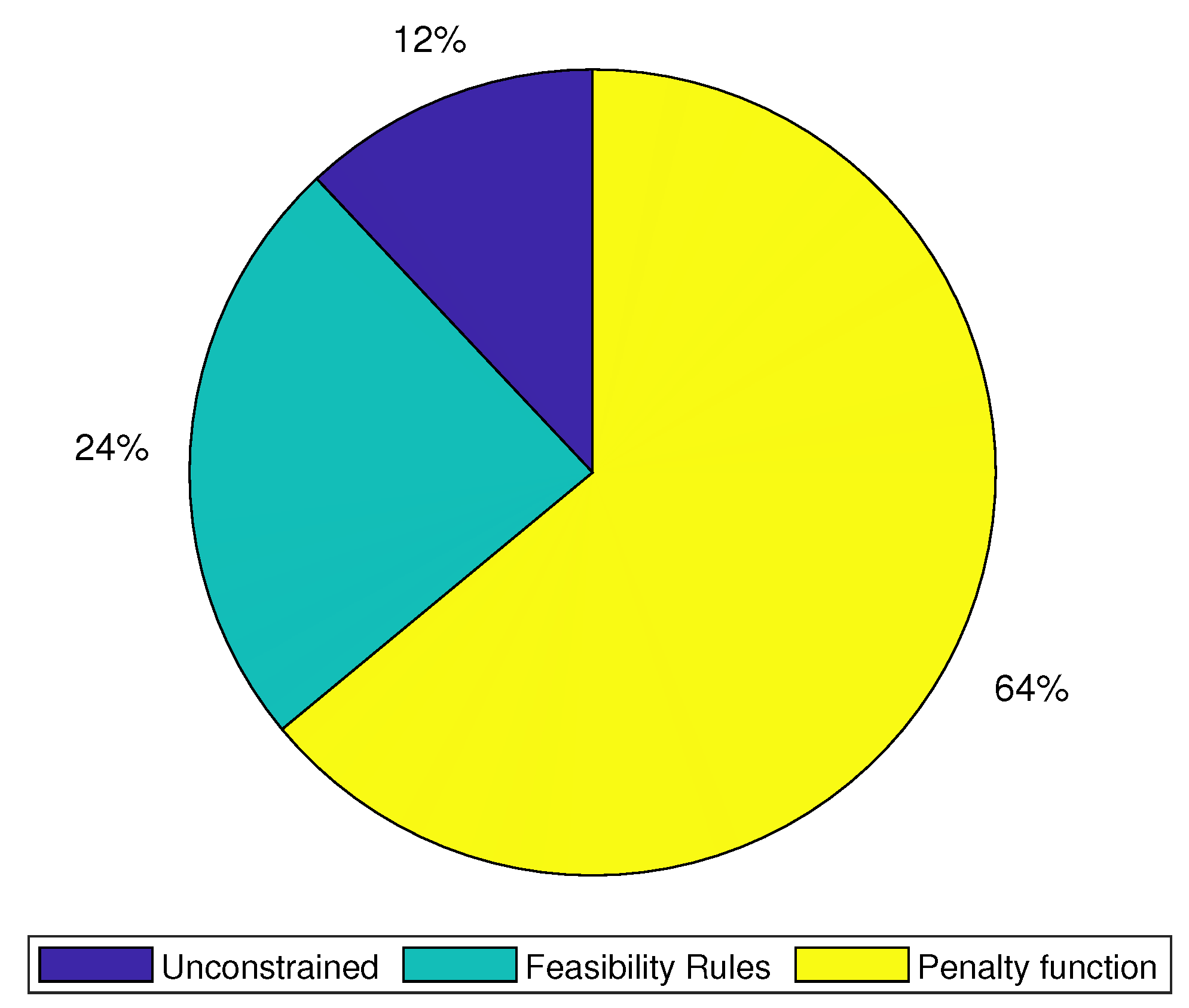
From the literature review regarding the design of closed-chain mechanisms for rehabilitation and the general framework of kinematic synthesis of mechanisms, both included in Table 1, the metaheuristic algorithms incorporate only one constraint-handling technique to solve the constraint optimization problem. Figure 1 shows the use of CHTs reported in the literature for the synthesis of mechanisms using metaheuristic algorithms. As observed in that figure, 64% of the reviewed literature uses the penalty functions, followed by the feasibility rules with a 24% of use.

Figure 1. Use of the constraint-handling techniques in the optimal synthesis of mechanisms with metaheuristic algorithms according to Table 1.

According to [37,39,41], the constraint-handling technique is an essential factor to solve constrained optimization problems because these techniques influence the exploration and exploitation capabilities of algorithms for the search of the most promising solution. However, other CHTs in the second generation, such as stochastic ranking and $ϵ$-constraint have not been evaluated in solving these types of problems.

Depending on the problem nature in the kinematic synthesis for rehabilitation (multimodality, types of functions, design variable space, and the feasible space ratio), the most frequently used algorithms and the constraint-handling techniques can be suitable during the search process of the metaheuristic algorithms. Nevertheless, the high interactions in the problem nature and the metaheuristic algorithms make it difficult to suggest a constraint-handling technique that is more likely to perform well against different algorithms.

Motivated by these facts, and to the best of the author’s knowledge, there is a gap in the comparative study of the performance of different constraint-handling techniques in the dimensional synthesis of mechanisms. This research can aid researchers or practitioners interested in applying metaheuristic algorithms in the kinematic synthesis of this kind of problem with insights about the quality and consistency of the obtained results in the studied CHTs and can identify the most promising CHT alternatives for the synthesis problems.

Thus, researchers and practitioners can have some basic knowledge in the analyzed CHTs about the likelihood of increasing the optimization efficiency and the consistency of the obtained results when those CHTs are included in different metaheuristic algorithms. Hence, this work can suggest the use of a particular CHT in the optimizers to achieve optimum kinematic synthesis.

Therefore, in this work, the performance of the penalty function, feasibility rules, stochastic-ranking, and $ϵ$-constraint is studied to solve three real-world engineering problems reported in the literature related to the synthesis of mechanisms for rehabilitation by using metaheuristic algorithms. In this study, ten metaheuristic algorithms commonly used in the synthesis of mechanisms for rehabilitation are implemented in such CHTs. These are eight variants of a differential evolution algorithm, a Genetic Algorithm (GA), and a Particle Swarm Optimization (PSO) algorithm.

The parameters of the algorithms are tuned using the irace package to make a fair comparison and provide useful insights about the studied CHTs. On the other hand, the four-bar linkage mechanism, the cam-linkage mechanism, and the eight-bar linkage mechanism are considered in the mechanism synthesis for rehabilitation.

This paper is organized as follows: In Section 2, the general problem of mechanism synthesis for rehabilitation is presented. Section 3 describes the metaheuristic algorithms and the constraint-handling techniques used in this study. Section 4 states three state-of-art synthesis problems for rehabilitation to be solved. In Section 5, the study of the constraint-handling techniques is presented and discussed. In addition, the best and worst solution are analyzed and compared. Finally, Section 6 presents our conclusions.

2. Optimization Problem Statement

In this work, optimization problems for the synthesis of rehabilitation mechanisms are studied. The synthesis problem usually requires satisfying more than one design objective and constraint. Therefore, the design problems can be considered as a Constrained Multiobjective Optimization Problem (CMOPs). According to literature related to the synthesis of mechanisms for rehabilitation presented in Table 1, it is observed that CMOPs are typically transformed into constrained mono-objective optimization problems by the weighted sum approach [42,43]. Hence, mono-objective optimization problems for the mechanism synthesis are only considered in this study. These are formally stated as follows:

$$\begin{array}{cc}& \underset{x}{\mathrm{Min}}\overline{J}\left(x\right)\\ \hfill \mathrm{subject}\mathrm{to}:\end{array}$$

(1)

$$\begin{array}{cc}& g_j\left(x\right)\le 0\forall j=\{1,2,\dots ,m\}\end{array}$$

(2)

$$\begin{array}{cc}& h_k\left(x\right)=0\forall k=\{1,2,\dots ,r\}\end{array}$$

(3)

$$\begin{array}{cc}& x_{min}\le x\le x_{max}\end{array}$$

(4)

where $\overline{J}\left(x\right)={\sum }_{i=1}^n{w}_i{J}_i\left(x\right)$ is the weighted objective function; $J_i$ is the $i-th$ design objective of the system; x is the design variable vector; $w_i$ is the $i-th$ weight attributed to each objective; n is the number of design objectives; $g_j\left(x\right)$ and $h_k\left(x\right)$ are the inequality and equality constraints, respectively; and $x_{min}$, $x_{max}$ are the design variable bounds.

3. Constraint-Handling Techniques in Metaheuristic Algorithms

Metaheuristic algorithms are optimization strategies used to solve a wide range of hard optimization problems. The metaheuristics are inspired by biological systems, social behaviors, among others.

In recent years, metaheuristic algorithms have been used to provide satisfactory solutions to optimization problems related to the mechanism synthesis, see Table 1. The behavior of metaheuristic algorithms to search for better solutions can be improved through suitable constraint handling. In this work, the behavior of four Constraint-Handling Techniques in different metaheuristic algorithms is studied. The CHTs [44] involve the Penalty Functions (PF), Feasibility Rules (FR), Stochastic Ranking (SR), and $ϵ$-Constraint ($ϵ$ C) method.

The considered metaheuristic algorithms are eight Differential Evolution variants [45], the Genetic Algorithm [46], and the Particle Swarm Optimization [47]. Those techniques and algorithms are frequently used in mechanism synthesis for rehabilitation and have provided satisfactory solutions, as is shown in Table 1. However, according to that table, differential evolution is one of the most promising reported optimizers. Therefore, the main DE variants [48] are analyzed in this study.

3.1. Metaheuristic Algorithms

3.1.1. Differential Evolution Algorithm

The DE algorithm was proposed by Storn and Price [45], and it is a direct and stochastic search method. DE was inspired by the theory of natural selection and is shown in the Algorithm 1.

Algorithm 1 Differential evolution pseudocode.
1:	Generate an initial population $X_0$ with $NP$ individuals.
2:	Evaluate $X_0$.
3:	Initialize the best individual $x_{best}$.
4:	$G\leftarrow 0$
5:	while$G\le G_{max}$do
6:	for all $x_i\in X_G$do
7:	Generate a child individual $u_i$ based on (5)–(12).
8:	Evaluate $u_i$ and $U_G\leftarrow u_i$.
9:	end for
10:	Select the new population $X_{G+1}$ between $X_G$ and $U_G$ according to CHT.
	$[X_{G+1},x^{\underset{swarm}{best}}]\leftarrow fncCHT(X_G,U_G,x_{best})$ (This function is associated to the CHT.)
11:	$G\leftarrow G+1$
12:	end while

DE starts with a population of individuals called parents $X_0=\{x_1,x_2,\dots ,x_{NP}\}$, where $NP$ is the number of individuals in the population. At each generation G, the individuals in the population $X_G$ perform a crossover and mutation process to generate a population of child individuals $U_G$. The crossover and mutation process depend on the used DE variant. In this case, eight DE variants are chosen, and these are: DE/rand/1/bin (DER1B), DE/rand/1/exp (DER1E), DE/best/1/bin (DEB1B), DE/best/1/exp (DEB1E), DE/current to rand (DECR), DE/current to best (DECB), DE/current to rand/1/bin (DECR1B), and DE/current to rand/1/exp (DECR1E).

The crossover and mutation process for each variant is defined by Equations (5)–(12), where $CR$ is the crossover factor, F and K are scale factors, $r_1$, $r_2$, and $r_3$ are three random individuals from the current population, D is the number of design variables and $j_{rand}\in \{1,2,\dots ,D\}$ is a random value that represents the crossover point.

Binomial recombination:

Rand/1/Bin:

$$\begin{array}{ccc}\hfill u_i^j& =& \left\{\begin{array}{cc}{x}_{r_3}^j+F(x_{r_1}^j-x_{r_2}^j),& \mathrm{if}{\mathrm{rand}}_{\mathrm{j}}(0,1)<\mathrm{CR}\mathrm{or}\mathrm{j}={\mathrm{j}}_{\mathrm{rand}}\\ x_i^j,& \mathrm{Otherwise}\end{array}\right.\hfill \end{array}$$

(5)

Best/1/Bin:

$$\begin{array}{ccc}\hfill u_i^j& =& \left\{\begin{array}{cc}{x}_{best}^j+F(x_{r_1}^j-x_{r_2}^j),& \mathrm{if}{\mathrm{rand}}_{\mathrm{j}}(0,1)<\mathrm{CR}\mathrm{or}\mathrm{j}={\mathrm{j}}_{\mathrm{rand}}\\ x_i^j& \mathrm{Otherwise}\end{array}\right.\hfill \end{array}$$

(6)

Exponential recombination:

Rand/1/Exp:

$$\begin{array}{ccc}\hfill u_i^j& =& \left\{\begin{array}{cc}{x}_{r_3}^j+F(x_{r_1}^j-x_{r_2}^j),& \mathrm{from}{\mathrm{rand}}_{\mathrm{j}}(0,1)<\mathrm{CR}\mathrm{or}\mathrm{j}={\mathrm{j}}_{\mathrm{rand}}\\ x_i^j,& \mathrm{Otherwise}\end{array}\right.\hfill \end{array}$$

(7)

Best/1/Exp:

$$\begin{array}{ccc}\hfill u_i^j& =& \left\{\begin{array}{cc}{x}_{best}^j+F(x_{r_1}^j-x_{r_2}^j),& \mathrm{from}{\mathrm{rand}}_{\mathrm{j}}(0,1)<\mathrm{CR}\mathrm{or}\mathrm{j}={\mathrm{j}}_{\mathrm{rand}}\\ x_i^j& \mathrm{Otherwise}\end{array}\right.\hfill \end{array}$$

(8)

Arithmetic recombination:

Current-to-Rand/1:

$$\begin{array}{ccc}\hfill {\overrightarrow{u}}_i& =& {\overrightarrow{x}}_i+K({\overrightarrow{x}}_{r_3}-{\overrightarrow{x}}_i)+F({\overrightarrow{x}}_{r_1}-{\overrightarrow{x}}_{r_2})\hfill \end{array}$$

(9)

     Current-to-Best/1:

$$\begin{array}{ccc}\hfill {\overrightarrow{u}}_i& =& {\overrightarrow{x}}_i+K({\overrightarrow{x}}_{best}-{\overrightarrow{x}}_i)+F({\overrightarrow{x}}_{r_1}-{\overrightarrow{x}}_{r_2})\hfill \end{array}$$

(10)

Arithmetic-binomial recombination:

Current-to-Rand/1/Bin:

$$\begin{array}{ccc}\hfill u_i^j& =& \left\{\begin{array}{cc}{x}_i^j+K(x_{r_3}^j-x_i^j)+F(x_{r_1}^j-x_{r_2}^j)\hfill & \mathrm{if}{\mathrm{rand}}_{\mathrm{j}}(0,1)<\mathrm{CR}\mathrm{or}\mathrm{j}={\mathrm{j}}_{\mathrm{rand}}\\ x_i^j\hfill & \mathrm{Otherwise}\end{array}\right.\hfill \end{array}$$

(11)

Current-to-Rand/1/Exp:

$$\begin{array}{ccc}\hfill u_i^j& =& \left\{\begin{array}{cc}{x}_i^j+K(x_{r_3}^j-x_i^j)+F(x_{r_1}^j-x_{r_2}^j)\hfill & \mathrm{if}{\mathrm{rand}}_{\mathrm{j}}(0,1)<\mathrm{CR}\mathrm{or}\mathrm{j}={\mathrm{j}}_{\mathrm{rand}}\\ x_i^j\hfill & \mathrm{Otherwise}\end{array}\right.\hfill \end{array}$$

(12)

The population of parents $X_G$ and children $U_G$ compete at each generation to remain to a new population of individuals $X_{G+1}$ for the next generation. The selection process between the parents and children is based on the CHT, as defined in Section 3.2. Then, the best individual in the population $X_{G_{max}}$ is considered the best solution for the optimization problem.

3.1.2. Particle Swarm Optimization

The PSO algorithm was proposed by Kennedy and Eberhart [47]. This algorithm is inspired by the collaborative behavior of species in search of food and is shown in Algorithm 2.

Algorithm 2 Particle swarm optimization pseudocode.
1:	Initialize the swarm position $u_i\in U_0$ with $NP$ particles.
2:	Evaluate the swarm $U_0$.
3:	Initialize the best known position $X_0=U_0$.
4:	Initialize the best position of the swarm $x^{\underset{swarm}{best}}$.
5:	Initialize the velocity of each particle $v_i\in V_0$.
6:	$G\leftarrow 0$
7:	while$G\le G_{max}$do
8:	Update the inertial weight w based on (13).
9:	for all $u_i\in U_G$do
10:	Update the velocity $v_i$ based on (14).
11:	Update the position $u_i$ based on (15).
12:	Evaluate $u_i$.
13:	end for
14:	Update the best known position $X_{G+1}$ and the best particle in the swarm $x^{\underset{swarm}{best}}$ with the use of CHT between $X_G$ and $U_G$.
	$[X_{G+1},x^{\underset{swarm}{best}}]\leftarrow fncCHT(X_G,U_G,x^{\underset{swarm}{best}})$ (This function is associated to the CHT.)
15:	$G\leftarrow G+1$
16:	end while

The PSO algorithm initializes with a swarm $U_{G=0}$ with $NP$ particles. Each particle is located in a position $u_i$ with a velocity $v_i$$\forall i=\{1,2,\dots ,NP\}$. The best known positions of the particles are saved in the swarm $X_{G=0}$. The best particle in the swarm $X_0$ is stored in $x^{\underset{swarm}{best}}$. In the time G (iteration), the $i-th$ position and velocity of each particle $u_i$ are updated by Equations (13)–(15), where w is the inertial weight, $v_{max}$ and $v_{min}$ are the maximum and minimum velocity values, $x^{best}$ is the best neighborhood particle of $x_i$ in a ring topology, and $C_1$, $C_2$ are weighting factors.   

$$w=v_{max}-\frac{G}{G_{max}}(v_{max}-v_{min})$$

(13)

$$v_i=w{v}_i+rand(0,1)C_1(x_i^{best}-x_i)+rand(0,1)C_2(x_i^{\underset{swarm}{best}}-x_i)$$

(14)

$$u_i=u_i+v_i$$

(15)

Finally, the best particle $x^{\underset{swarm}{best}}$ and the best particles positions $X_G$ are updated considering the CHT as is defined in Section 3.2. Then, the best solution is found in $x^{\underset{swarm}{best}}$.

3.1.3. Genetic Algorithm

The GA was proposed by John Henry Holland [49]. This algorithm is inspired by genetic-molecular evolution. The essential operation of GA is shown in Algorithm 3.

Algorithm 3 Genetic algorithm pseudocode.
1:	Generate a initial population $X_0$ with $NP$ chromosomes.
2:	Evaluate $X_0$
3:	$G\leftarrow 0$
4:	while$G\le G_{max}$do
5:	for all  $x_i\in X_G$do
6:	Obtain $x_{r_1}$ and $x_{r_2}$ in $X_G$ by tournament.
7:	Generate a child $v_i$ by (16)
8:	Generate a mutant $u_i$ by (17)
9:	Evaluate $u_i$
10:	end for
11:	Replace the population $X_G$ to $X_{G+1}$ considering $X_G$ and $U_G$ in the CHT.$X_{G+1}\leftarrow fncCHT(X_G,U_G,\sim )$ (This function is associated to the CHT.)
12:	$G\leftarrow G+1$
13:	end while

GA initializes with a group $X_0=\{x_1,x_2,\dots ,x_{NP}\}$ of $NP$ chromosomes. In the group, two parent chromosomes $x_{r_1}$ and $x_{r_2}$ are selected by tournament [50] and recombined to generate a child chromosome $v_i$ as shown in (16). The recombination process uses a piece-wise multipoint crossover [5], where the crossover points are given by a crossover rate $CR\in [0,1]$. The child chromosome $v_i$ can mute using uniform mutation [51] as shown in (17), where $MR\in [0,1]$ is a mutation rate, and $x_{min}^j$, $x_{max}^j$ are the minimum and maximum values of the design variables, respectively.

$$v_i^j=\left\{\begin{array}{cc}{x}_{r_1}^j,& \mathrm{if}{\mathrm{rand}}_{\mathrm{j}}(0,1)<\mathrm{CR}\\ x_{r_2}^j,& \mathrm{Otherwise}\end{array}\right.$$

(16)

$$u_i^j=\left\{\begin{array}{cc}rand(x_{min}^j,x_{max}^j),& \mathrm{if}{\mathrm{rand}}_{\mathrm{j}}(0,1)<\mathrm{MR}\\ v_i^j,& \mathrm{Otherwise}\end{array}\right.$$

(17)

Between the mutant chromosomes $U_G$ and the parent one $X_G$, the best chromosomes are selected based on the replacement mechanism using the CHT defined in Section 3.2.

3.2. Constraint-Handling Techniques

Metaheuristic algorithms have been used to solve complex optimization problems. In their original versions, these have been designed to solve unconstrained optimization problems. However, optimization problems in engineering usually have constraints. Currently, constraint-handling techniques, such as the PF, FR, SR, and $ϵ$ C method, have been the most popular techniques to solve constrained optimization problems [44]. Each one of these techniques is described below.

3.2.1. Penalty Function

The PF [52] has been frequently used to solve constrained optimization problems in the mechanism synthesis. The PF transforms an optimization problem with constraints into an unconstrained problem. The most used transformation equation is:

$${\overline{J}}^{\prime }\left(x\right)=\stackrel{\overline{J}}{\overbrace{{\sum }_{i=1}^n{w}_i{J}_i\left(x\right)}}+\stackrel{Penaltyterm}{\overbrace{{\sum }_{j=1}^m{\varpi }_j{\gamma }_j\left(x\right)}}$$

(18)

where ${\overline{J}}^{\prime }\left(x\right)$ is the new function to minimize, $\overline{J}$ is the weighted objective function, x is the vector of design variables, m is the number of constraints, ${\gamma }_j\left(x\right)$ is the infeasible constraint distance defined by (19), and ${\varpi }_j$ is the penalty factor that can be static, dynamic, or adaptive. In engineering optimization problems, the term ${\varpi }_j$ is usually defined with a static value.

$${\gamma }_j\left(x\right)=max(0,g_j\left(x\right))$$

(19)

Algorithm 4 describes the operation of PF. This constraint-handling technique requires three sets of solutions (three input arguments). At each iteration G, those solutions are compared according to the new function ${\overline{J}}^{\prime }\left(x\right)$ (18). The best solutions are stored in the output arguments.

Algorithm 4 Penalty function pseudocode.

1: Function $fncCHT(\tilde{a},\tilde{b},\tilde{c})$ Input: $\tilde{a}\in X_G$ and $\tilde{b}\in U_G$ Output: $X_{G+1}$ and $x^{best}$ 2: $X_{G+1}=\tilde{a}$ and $x^{best}=\tilde{c}$ 3: for$i=1$ to $NP$ do 4:  if${\overline{J}}^{\prime }\left({\tilde{b}}_i\right)<{\overline{J}}^{\prime }\left({\tilde{a}}_i\right)$then 5:   $X_{G+1}\leftarrow {\tilde{b}}_i$ 6:   if${\overline{J}}^{\prime }\left({\tilde{b}}_i\right)<{\overline{J}}^{\prime }\left(x^{best}\right)$then 7:     $x^{best}\leftarrow {\tilde{b}}_i$ 8:   end if 9:  end if 10: end for

3.2.2. Feasibility Rules

The FR were proposed by Deb [53]. Three rules define this constraint-handling technique, these are:

• Between two infeasible solutions, the solution with the fewest number of violated constraints is chosen.
• Between a feasible solution and an infeasible one, the feasible solution is chosen.
• Among two feasible solutions, the solution with the best objective function is chosen.

In this work, the number of violated constraints is considered the sum of infeasible constraint distance $\varphi \left(x\right)$ and shown in (20).

$$\varphi \left(x\right)=\sum _{j=1}^{m}max(0,g_j\left(x\right))$$

(20)

Algorithm 5 describes the operation of FR. This constraint-handling technique requires three sets of solutions (three input arguments). At each iteration G, those solutions are compared according to the feasibility rules. Finally, the best solutions are stored in the output arguments.

Algorithm 5 Feasibility rules pseudocode.

1: Function $fncCHT(\tilde{a},\tilde{b},\tilde{c})$

Input: $\tilde{a}\in X_G$ and $\tilde{b}\in U_G$

Output: $X_{G+1}$ and $x^{best}$ 2: $X_{G+1}=\tilde{a}$ and $x^{best}=\tilde{c}$ 3: for$i=1$ to $NP$ do 4:  if ($\varphi \left({\tilde{a}}_i\right)>0$ and $\varphi \left({\tilde{b}}_i\right)>0$ and $\varphi \left({\tilde{b}}_i\right)<\varphi \left({\tilde{a}}_i\right)$) or  ($\varphi \left({\tilde{a}}_i\right)>0$ and $\varphi \left({\tilde{b}}_i\right)==0$) or ($\varphi \left({\tilde{a}}_i\right)==0$ and $\varphi \left({\tilde{b}}_i\right)==0$ and $\overline{J}\left({\tilde{b}}_i\right)<\overline{J}\left({\tilde{a}}_i\right)$) then 5:    $X_{G+1}\leftarrow {\tilde{b}}_i$ 6:   if ($\varphi \left(x^{best}\right)>0$ and $\varphi \left({\tilde{b}}_i\right)>0$ and $\varphi \left({\tilde{b}}_i\right)<\varphi \left(x^{best}\right)$) or ($\varphi \left(x^{best}\right)>0$ and $\varphi \left({\tilde{b}}_i\right)==0$) or ($\varphi \left(x^{best}\right)==0$ and $\varphi \left({\tilde{b}}_i\right)==0$ and $\overline{J}\left({\tilde{b}}_i\right)<\overline{J}\left(x^{best}\right)$) then 7:     $x^{best}\leftarrow {\tilde{b}}_i$ 8:   end if 9:  end if 10: end for

3.2.3. $ϵ$-Constraint Method

The $ϵ$ C method was proposed by Takahama et al. [54]. This method relaxes the constraints to select solutions close to the feasible region. The selection process is described by (21).

$$(\overline{J}\left(x_1\right),\varphi \left(x_1\right)){<}_{ϵ}(\overline{J}\left(x_2\right),\varphi \left(x_2\right))\left\{\begin{array}{c}\overline{J}\left(x_1\right)<\overline{J}\left(x_2\right),\mathrm{if}\varphi \left(x_1\right),\varphi \left(x_2\right)\le ϵ\\ \overline{J}\left(x_1\right)<\overline{J}\left(x_2\right),\mathrm{if}\varphi \left(x_1\right)==\varphi \left(x_2\right)\\ \varphi \left(x_1\right)<\varphi \left(x_2\right),\mathrm{otherwise}\end{array}\right.$$

(21)

where $ϵ$ is a relaxation factor defined by (22) and (23), $cp$ is a parameter to control the speed of reducing relaxation of constraints, $T_c$ is the maximum number of iterations (generation or time) to relax such constraints, $\varphi \left(x_{\theta }\right)$ is $\theta$-th best value of the objective function in the initial solution vector (population, swarm, or chromosomes).

$$\begin{array}{ccc}\hfill ϵ\left(0\right)& =& \varphi \left(x_{\theta }\right)\hfill \end{array}$$

(22)

$$\begin{array}{ccc}\hfill ϵ\left(G\right)& & \left\{\begin{array}{cc}ϵ\left(0\right){\left(1-\frac{1}{T_c}\right)}^{cp},& 0<G<Tc\\ 0,& Tc\le G\end{array}\right.\hfill \end{array}$$

(23)

The $ϵ$-constraint method finds feasible regions using the gradient of constraints at an infeasible region. Algorithm 6 describes the operation of the $ϵ$ C method. This constraint-handling technique requires three sets of solutions (three input arguments). The gradient-based mutation process can improve an infeasible solution to obtain a new solution $u_j^{new}$. The new solution $u_j^{new}$ and old solution are compared using (21), and the best solution is stored in the current solution $b_j$. The set of current solutions are compared according to (21), and the best solutions are stored in the output arguments.

Algorithm 6$ϵ$-constraint method pseudocode.
1:	Function $fncCHT(\tilde{a},\tilde{b},\tilde{c})$
	Input: $\tilde{a}\in X_G$ and $\tilde{b}\in U_G$
	Output: $X_{G+1}$ and $x^{best}$
2:	$X_{G+1}=\tilde{a}$ and $x^{best}=\tilde{c}$
3:	for$j=1$ to $NP$ do
4:	if$rand(0,1)<Pg$then
5:	$k=0$
6:	while $k<Rg$ and $\varphi \left({\tilde{b}}_j\right)>ϵ$ do
7:	Obtain $\Delta {\tilde{b}}_j=-\nabla C{\left({\tilde{b}}_j\right)}^{-1}\Delta C\left({\tilde{b}}_j\right)$
	$\Delta C\left({\tilde{b}}_j\right)$ is the constraint vector, $\Delta C{\left({\tilde{b}}_j\right)}^{-1}$ is the pseudo-inverse of the constraint’s derivative obtained by Moore–Penrose pseudo-inverse using the singular value decomposition and $Rg$ is the number of attempts to improve the solution.
8:	Obtain $u^{new}={\tilde{b}}_j+\Delta {\tilde{b}}_j$
9:	if$(\overline{J}\left(u^{new}\right),\varphi \left(u^{new}\right)){<}_{ϵ}(\overline{J}\left({\tilde{b}}_j\right),\varphi \left({\tilde{b}}_j\right))$then
10:	${\tilde{b}}_j\leftarrow u^{new}$
11:	else
12:	$break$
13:	end if
14:	$k=k+1$
15:	end while
16:	end if
17:	if$(\overline{J}\left({\tilde{b}}_j\right),\varphi \left({\tilde{b}}_j\right)){<}_{ϵ}(\overline{J}\left({\tilde{a}}_j\right),\varphi \left({\tilde{a}}_j\right))$then
18:	$X_{G+1}\leftarrow b_j$
19:	if$(\overline{J}\left({\tilde{b}}_j\right),\varphi \left({\tilde{b}}_j\right)){<}_{ϵ}(\overline{J}\left(x^{best}\right),\varphi \left(x^{best}\right))$then
20:	$x^{best}\leftarrow b_j$
21:	end if
22:	end if
23:	end for

3.2.4. Stochastic-Ranking

SR was proposed by Runarsson and Yao [55]. This constraint-handling technique makes the pseudo-random sort of solutions. The ranking of solutions is based on the bubble sort algorithm with a probabilistic factor $Pf\in [0,1]$. The values close to zero in $Pf$ mean a high probability that the sort is based on the constraint distance. On the contrary, this is based on the objective function.

Algorithm 7 describes the operation of SR. This constraint-handling technique requires two sets of solutions (two input arguments). At each iteration G, those solutions are compared and stochastically ranked. The best first NP solutions in the ranking are stored in the output arguments.

Algorithm 7 Stochastic ranking pseudocode.

1: Function $fncCHT(\tilde{a},\tilde{b},\sim )$

Input: $\tilde{a}\in X_G$ and $\tilde{b}\in U_G$

Output: $X_{G+1}$ and $x^{best}$ 2: Obtain ${\widehat{X}}_G=\tilde{a}\cup \tilde{b}$ 3: for$i=2$ to $2NP$ do 4:  for $j=1$ to $2NP-i$ do 5:   if $\varphi \left({\widehat{x}}_j\right)=\varphi \left({\widehat{x}}_{j+1}\right)=0$ or $rand(0,1)<Pf$ then 6:    if $\overline{J}\left({\widehat{x}}_j\right)>\overline{J}\left({\widehat{x}}_{j+1}\right)$then 7:      $swap({\widehat{x}}_j,{\widehat{x}}_{j+1})$ 8:    end if 9:   else 10:    if $\varphi \left({\widehat{x}}_j\right)>\varphi \left({\widehat{x}}_{j+1}\right)$then 11:      $swap({\widehat{x}}_j,{\widehat{x}}_{j+1})$ 12:    end if 13:   end if 14:  end for 15:  if No swap then 16:    $break$ 17:  end if 18:   $X_{G+1}\leftarrow \{{\widehat{x}}_j\in {\widehat{X}}_G|j=1,2,\dots ,NP\}$ 19:   $x^{best}\leftarrow {\widehat{x}}_1\in {\widehat{X}}_G$ 20: end for

4. Study Cases in the Mechanism Synthesis for Lower Limb Rehabilitation

In this work, three study cases in engineering related to the mechanism design for the rehabilitation of lower limbs are considered for testing four constraint-handling techniques in different metaheuristic algorithms. Case 1 is related to a four-bar linkage mechanism, Case 2 involves a cam-linkage mechanism, and Case 3 includes an eight-bar linkage mechanism. Each study case is described below.

4.1. Case 1: Four-Bar Linkage Mechanism

The four-bar linkage mechanism has been used in lower limb rehabilitation for adults and children with cerebral palsy [9,16]. The dimensional synthesis design problem consists of finding the link lengths that approximate the coordinates $[x_P^i,y_P^i]$ of the coupler link point P to the coordinates $[{\overline{x}}_P^i,{\overline{y}}_P^i]$ of the ankle trajectory in a standard gait cycle. The schematic representation of the four-bar mechanism is presented in Figure 2.

Figure 2. Four-bar linkage mechanism.

According to Figure 2, the vector of design variables comprises the lengths of the links $r_1$, $r_2$, $r_3$, $r_4$, the ground link angle ${\theta }_1$, the initial position of the mechanism [$x_0$,$y_0$] with respect to the coordinate system $x-y$, and the crank angles ${\theta }_2^i\forall i=\{1,2,\dots ,n_f\}$. The vector of design variables is defined as:

$$x=\left[\begin{array}{c}{r}_1,r_2,r_3,r_4,{\theta }_1,x_0,y_0,r_{c_x},r_{c_y},{\theta }_2^1,{\theta }_2^2,\dots ,{\theta }_2^{n_f}\end{array}\right]$$

(24)

The optimization problem for the dimensional synthesis of the mechanism is presented in (25)–(29), where the constant values $w_1=1$ and $w_2=0.01$ weight the design goals.

$$\underset{x}{\mathrm{Min}}{w}_1\sum _{i=1}^{n_f}[{(x_P^i-{\overline{x}}_P^i)}^2+{(y_P^i-{\overline{y}}_P^i)}^2]+w_2\sum _{i=1}^{n_f}{({\theta }_2^i-{\overline{\theta }}_2^i)}^2$$

(25)

subject to:

$$\begin{array}{ccc}& & g_1\left(x\right)\le 0:r_2+r_1-r_3-r_4\le 0\hfill \end{array}$$

(26)

$$\begin{array}{ccc}& & g_2\left(x\right)\le 0:-r_4-r_1+r_2+r_3\le 0\hfill \end{array}$$

(27)

$$\begin{array}{ccc}& & g_3\left(x\right)\le 0:-r_3-r_1+r_2+r_4\le 0\hfill \end{array}$$

(28)

$$\begin{array}{ccc}& & x_{min}\le x\le x_{max}\hfill \end{array}$$

(29)

The first design goal refers to the error between the desired precision points $[{\overline{x}}_P^i,{\overline{y}}_P^i]$ related to the ankle trajectory and the path $[x_P^i,y_P^i]$ of the mechanism’s coupler link point. The second design goal refers to the angular displacement error between the desired angles ${\overline{\theta }}_2^i$ and the crank angles ${\theta }_2^i$. In this problem, the desired angles ${\overline{\theta }}_2^i$ are defined by (30).

$$\begin{array}{cc}& \overline{{\theta }_2^i}={\theta }_2^1+2\pi \frac{i-1}{n_f-1}\forall i=\{1,2,\dots ,n_f\}\end{array}$$

(30)

The precision (desired) points $[{\overline{x}}_P^i,{\overline{y}}_P^i]$ are defined based on the standard ankle trajectory, these points are shown in Table A1 of Appendix A, and are obtained in [16]. On the other hand, according to Figure 2, the points generated by the coupler link $[x_P^i,y_P^i]$ are defined by (31), where ${\theta }_2$ is the angle of the crank link (input link), and ${\theta }_3$ is shown in (32). This is obtained by the Freudenstein equation. It is important to note that both solutions in ${\theta }_3$ (related to the sign of the root) are computed, and the solution that provides a better objective function is chosen. Thus, with the selection of ${\theta }_3$, the resulting mechanism can be an open (+) and crossed (−) four-bar mechanism.

$$\left[\begin{array}{c}{x}_P\\ y_P\end{array}\right]=\left[\begin{array}{c}{x}_0+r_{2}cos{\theta }_2+r_{c_x}cos{\theta }_3-r_{c_y}sin{\theta }_3\\ y_0+r_{2}sin{\theta }_2+r_{c_x}sin{\theta }_3+r_{c_y}cos{\theta }_3\end{array}\right]$$

(31)

$${\theta }_3=2atan2\left(-B\pm \sqrt{B^2+A^2-C^2},C-A\right)$$

(32)

where $A=-2r_1{r}_{3}cos{\theta }_1+2r_2{r}_{3}cos{\theta }_2$, $B=-2r_1{r}_{3}sin{\theta }_1+2r_2{r}_{3}sin{\theta }_2$, and $C=r_1^2+r_2^2+r_3^2-r_4^2-2r_1{r}_{2}cos({\theta }_1-{\theta }_2)$.

The design problem has three inequality constraints (26)–(28) that define a crank-rocker mechanism according to the Grashof criterion [56]. The design variables vector $x\in R^{23}$ is bounded by its corresponding limit $x_{min}$ and $x_{max}$. In Table 2 the limit values used in this work are shown. These values are obtained by [16].

Table 2. The maximum and minimum parameters of the x vector for the four-bar mechanism.

x	Parameter	${\mathit{x}}_{\mathit{min}}$	${\mathit{x}}_{\mathit{max}}$
$x_1-x_4$	$r_1-r_4$	0 [m]	0.6 [m]
$x_5$	${\theta }_1$	0[rad]	$2\pi$ [rad]
$x_6-x_9$	$x_0,y_0$	$-0.6$ [m]	0.6 [m]
$x_{10}-x_{24}$	${\theta }_2^1-{\theta }_2^{14}$	$-\pi$ [rad]	$\pi$ [rad]

4.2. Case 2: Cam-Linkage Mechanism

The second optimization problem is related to the synthesis of a cam-linkage mechanism. The original design problem was presented by Yixin Shao et al. [15]. This mechanism is designed to provide rehabilitation routines for adults with motor problems in the lower limbs. The schematic diagram of the cam-linkage mechanism is shown in Figure 3.

Figure 3. Cam-linkage mechanism.

The design variable vector (33) is defined by the link lengths $r_1,r_2,\dots ,r_8$, the angles $\beta ,\gamma$, $\eta$, the initial position of the mechanism $[x_0,y_0]$ with respect to the $x-y$ coordinate system, and the position of the slide displacement axis defined by the length e and the angle $\alpha$.

$$x=\left[r_1,r_2,r_3,r_4,r_5,r_6,r_7,r_8,\alpha ,\beta ,\gamma ,\eta ,x_0,y_0,e\right]$$

(33)

The synthesis problem is presented in (34)–(46).

$$\underset{x}{\mathrm{Min}}{w}_1\frac{{\sum }_{i=1}^{n_f}{({\theta }_1^i-{\overline{\theta }}_1^i)}^2}{{\Theta }_{ref}}+w_2\frac{R_0}{R_{ref}}$$

(34)

subject to:

$$\begin{array}{cc}\hfill g_1& :r_1+r_2-r_3-\sqrt{s_{min}^2+e^2}\le 0\end{array}$$

(35)

$$\begin{array}{cc}\hfill g_2& :r_1+r_3-r_2-\sqrt{s_{min}^2+e^2}\le 0\end{array}$$

(36)

$$\begin{array}{cc}\hfill g_3& :r_1+\sqrt{s_{max}^2+e^2}-r_2-r_3\le 0\end{array}$$

(37)

$$\begin{array}{cc}\hfill g_4& :r_2^2+r_3^2-{\left(d_{AC}\right)}_{min}^2-2r_2{r}_{3}cos\pi /6\le 0\\ \hfill g_5& :-r_2^2-r_3^2+{\left(d_{AC}\right)}_{max}^2+\end{array}$$

(38)

$$\begin{array}{cc}& 2r_2{r}_{3}cos(\pi -\pi /6)\le 0\end{array}$$

(39)

$$\begin{array}{cc}\hfill g_6& :r_5^2+r_6^2-{\left(d_{DF}\right)}_{min}^2-2r_5{r}_{6}cos\pi /6\le 0\\ \hfill g_7& :-r_5^2-r_6^2+{\left(d_{DF}\right)}_{max}^2+\end{array}$$

(40)

$$\begin{array}{cc}& 2r_5{r}_{6}cos(\pi -\pi /6)\le 0\end{array}$$

(41)

$$\begin{array}{cc}\hfill g_8& :{\left(d_{OD}\right)}_{max}-r_4-r_1\le 0\end{array}$$

(42)

$$\begin{array}{cc}\hfill g_9& :|r_4-r_1|-{\left(d_{OD}\right)}_{min}\le 0\end{array}$$

(43)

$$\begin{array}{cc}\hfill g_{10}& :{\left(d_{Be}\right)}_{max}-r_3\le 0\end{array}$$

(44)

$$\begin{array}{cc}\hfill g_{11}& :0.12R_0-0.6{\left|\rho \right|}_{min}\le 0\end{array}$$

(45)

$$\begin{array}{cc}& x_{min}\le x\le x_{max}\end{array}$$

(46)

The first term of the weighted objective function (34) refers to the error between the crank angles ${\theta }_1^i\forall i=\{1,2,\dots ,n_f\}$ and the desired angles ${\overline{\theta }}_1^i\forall i=\{1,2,\dots ,n_f\}$, where $n_f$ is the number of precision points, and ${\overline{\theta }}_1^i$ is defined by Equation (47).

$$\overline{{\theta }_1^i}={\theta }_1^1+2\pi \frac{i-1}{n_f-1}\forall i=\{1,2,\dots ,n_f\}$$

(47)

On the other hand, the second term refers to the base radius $R_0$ of the cam (see Figure 3). Both design objectives are weighted by $w_1=0.3$ and $w_2=0.7,$ and normalized by ${\Theta }_{ref}=0.4246$ [rad] and $R_{ref}=0.3782$ [m] according to the best results presented in [15].

To guarantee the functionality of the mechanism, the design problem has inequality constraints. The first three constraints (35)–(37) guarantees a complete revolution of the crank angle ${\theta }_2$ (Grashof criterion), where $s_{min}$ and $s_{max}$ are the minimum and maximum values of $s\left({\theta }_1\right)$ in the precision points. The $s\left({\theta }_1\right)$ is given in (48) and is visualized in Figure 3.

$$s\left({\theta }_1\right)=r_{1}cos({\theta }_1-\alpha )+r_{2}cos({\theta }_2-\alpha )+\sqrt{r_3^2-{(r_{1}sin({\theta }_1-\alpha )+r_{2}sin({\theta }_2-\alpha )+e)}^2}$$

(48)

The next inequality constraints (38)–(41) provide high efficiency of the force transmission from the input link (crank link) to the output link, where the distances between point A to C $d_{AC}$, and between point D to F $d_{DF}$ are obtained by (49) and (50), respectively.

$$\begin{array}{c}\hfill d_{AC}=\sqrt{\begin{array}{c}{(r_{1}cos{\theta }_1-esin\alpha -scos\alpha )}^2+{(r_{1}sin{\theta }_1+ecos\alpha -ssin\alpha )}^2\end{array}}\end{array}$$

(49)

$$\begin{array}{c}\hfill d_{DF}=\sqrt{\begin{array}{c}{(x_D-x_0-r_{7}cos\beta )}^2+{(y_D-y_0-r_{7}sin\beta )}^2\end{array}}\end{array}$$

(50)

The inequality constraints (42)–(44) guarantee the path feasibility in the output link, where the distances between point D to F $d_{OD}$, and between point B to e $d_{Be}$ are obtained by (51) and (52), respectively.

$$\begin{array}{ccc}\hfill d_{OD}& =& \sqrt{{(x_D-x_0)}^2+{(y_D-y_0-)}^2}\hfill \end{array}$$

(51)

$$\begin{array}{ccc}\hfill d_{Be}& =& \sqrt{(y_B-y_0)cos\alpha -(x_B-x_0)sin\alpha +ϵ}\hfill \end{array}$$

(52)

The last inequality constraint (45) defines the minimum curvature radius of the cam profile. Moreover, the design variable vector x is bounded by $x_{min}$ and $x_{max}$. The limit values used in this work are shown in Table 3.

Table 3. The maximum and minimum parameters of the vector x for the cam-linkage mechanism.

x	${\mathit{x}}_{\mathit{min}}$	${\mathit{x}}_{\mathit{max}}$		x	${\mathit{x}}_{\mathit{min}}$	${\mathit{x}}_{\mathit{max}}$
$x_1$	0.1 [m]	0.4 [m]		$x_9$	−2.0944 [rad]	2.0944 [rad]]
$x_2$	0.3 [m]	0.6 [m]		$x_{10}$	−1.0472 [rad]	3.1416 [rad]
$x_3$	0.4 [m]	0.9 [m]		$x_{11}$	−1.0472 [rad]	3.1416 [rad]
$x_4$	0.3 [m]	0.7 [m]		$x_{12}$	−2.0944 [rad]	2.0944 [rad]
$x_5$	0.4 [m]	0.8 [m]		$x_{13}$	−0.5 [m]	0.5 [m]
$x_6$	0.3 [m]	0.7 [m]		$x_{14}$	−0.7 [m]	0.3 [m]
$x_7$,$x_8$	0.3 [m]	0.8 [m]		$x_{15}$	−0.2 [m]	0.2 [m]

The precision points $({\overline{x}}_P^i,{\overline{y}}_P^i)$ are presented in Table A2 of Appendix A. These coordinates define the standard ankle trajectory in the human gait. The precision points are obtained by the leg kinematics (53) considering an angular displacement of the hip and knee joint in the sagittal plane. The thigh and shank lengths are defined as $L_{thigh}=0.3984$ [m], $L_{shank}=0.3956$ [m], respectively. The knee angles ${\theta }_{knee}^i$ and the hip angles ${\theta }_{hip}^i$$\forall i=\{1,2,\dots ,n_f\}$ are found in [57].

$$\left[\begin{array}{c}{\overline{x}}_P^i\\ {\overline{y}}_P^i\end{array}\right]=\left[\begin{array}{cc}-sin{\theta }_{hip}^i& sin({\theta }_{knee}^i-{\theta }_{hip}^i)\\ -cos{\theta }_{hip}^i& -cos({\theta }_{knee}^i-{\theta }_{hip}^i)\end{array}\right]\left[\begin{array}{c}{L}_{thigh}\\ L_{shank}\end{array}\right]$$

(53)

The computation of the displacement angle ${\theta }_1^i$ and the cam radius $R_0$ in the optimization problem are obtained by inverse kinematics analysis of the mechanism. Therefore, $R_0$ is given in (54) and ${\theta }_1^i$ in (55).

$$\begin{array}{ccc}\hfill R_0& =& max\left(\sqrt{{\left(\frac{dh\left({\theta }_1\right)/d{\theta }_1\mp e}{tan\pi /6}-h\left({\theta }_1\right)\right)}^2+e^2}\right)\hfill \end{array}$$

(54)

$$\begin{array}{ccc}\hfill {\theta }_1& =& 2atan2\left(-{\tilde{B}}_2\pm \sqrt{{\tilde{B}}_2^2+{\tilde{A}}_2^2-{\tilde{C}}_2^2},{\tilde{C}}_2-{\tilde{A}}_2\right)\hfill \end{array}$$

(55)

where

$$\begin{array}{cc}& h\left({\theta }_1\right)=s\left({\theta }_1\right)-s_{min}\hfill \\ & {\theta }_2=atan2\left(\frac{y_D-r_{1}sin{\theta }_1-y_0}{x_D-r_{1}cos{\theta }_1-x_0}\right)-\eta \hfill \\ & {\tilde{A}}_2=-2r_1(x_D-x_0)\hfill \\ & {\tilde{B}}_2=-2r_1(y_D-y_0)\hfill \\ & {\tilde{C}}_2=r_1^2-r_4^2+{(y_D-y_0)}^2+{(x_D-x_0)}^2\hfill \\ & x_D=x_P+r_{8}cos(\pi +{\phi }_2-\gamma )+r_{5}cos\left({\phi }_2\right)\hfill \end{array}$$

$$\begin{array}{cc}& y_D=x_P+r_{8}sin(\pi +{\phi }_2-\gamma )+r_{5}sin\left({\phi }_2\right)\hfill \\ & {\phi }_2=2atan2\left(\frac{{\tilde{B}}_1\pm \sqrt{{\tilde{A}}_1^2+{\tilde{B}}_1^2-{\tilde{C}}_1^2}}{{\tilde{A}}_1+{\tilde{C}}_1}\right)+\gamma \hfill \\ & {\tilde{A}}_1=2r_8({\overline{x}}_P-x_0-r_{7}cos\beta )\hfill \\ & {\tilde{B}}_1=2r_8({\overline{y}}_P-y_0-r_{7}sin\beta )\hfill \\ & {\tilde{C}}_1=r_8^2-r_6^2+{(x_p-x_0-r_{7}cos\beta )}^2+{(y_p-y_0-r_{7}sin\beta )}^2\hfill \end{array}$$

The above equations are obtained according to the original design problem [15]. Except for the Equation (55), which is rewritten in this work from a two-argument arctangent. Equation (55) has two solutions that define the direction of crank rotation ${\theta }_1$. In this case, the clockwise turn in the crank link is chosen. Then, the solution in (55) that presents a positive increment between two different consecutive crank positions is selected.

On the other hand, the cam profile is obtained in (56) with respect to the coordinate system $x_0-y_0$.

$$\rho =\left[\begin{array}{c}ecos(\alpha -{\theta }_1)-\left(\sqrt{R_0^2-e^2}+h\left({\theta }_1\right))\right)sin(\alpha -{\theta }_1)\\ esin(\alpha -{\theta }_1)+\left(\sqrt{R_0^2-e^2}+h\left({\theta }_1\right))\right)cos(\alpha -{\theta }_1)\end{array}\right]$$

(56)

4.3. Case 3: Eight-Bar Linkage Mechanism

Case 3 includes an eight-bar linkage mechanism for rehabilitation of the lower limbs. This mechanism has been designed for rehabilitation routines for the average anthropometry for the Mexican population [3]. The integration among the kinematic synthesis, the link shape design, and the mechanism dynamics are considered for its design. The schematic diagram of the mechanism is displayed in Figure 4a.

Figure 4. Eight-bar linkage mechanism and the link shape.

According to Figure 4a, the design variables vector x is defined by (57).

$$x=[{\tilde{p}}_{ki},{\tilde{p}}_{sh}]\in R^{107}$$

(57)

This vector is split into two kinds of parameters, the kinematic parameter vector ${\tilde{p}}_{ki}=[l_1,l_2,\dots ,l_9,l_6^{\prime },$$l_8^{\prime },{\theta }_1,{\theta }_9,{\widehat{\theta }}_6$, ${\widehat{\theta }}_8,x_{ini},y_{ini},{\theta }_2^1,{\theta }_2^2,\dots ,{\theta }_2^{n_f}{]}^T\in R^{17+n_f}$ and the shape parameter vector ${\tilde{p}}_{sh}=[b_2,\dots ,b_8$, $c_2,\dots ,c_8,d_2,\dots ,d_8,e_2,\dots ,e_8,f_2,\dots ,f_8,g_2,$$\dots ,g_8,h_2,\dots ,h_8,$$i_2,\dots ,i_8,j_2,\dots ,j_8,$$k_2,\dots$, $k_8{]}^T\in R^{70}$. The shape parameters define the octagonal link shape shown in Figure 4b and the link dynamic parameters, such as the masses, the mass centers, and the inertia of links.

The synthesis problem for the eight-bar linkage mechanism is presented in (58)–(84).

The design objectives in (58) are weighted by parameters $w_1=1$ and $w_2=1e-6$. The first term refers to the average error between the precision points $({\overline{x}}_E^i,{\overline{y}}_E^i)$ and the points $(x_E^i,y_E^i)$ generated by the mechanism’s coupler link. The desired precision points $[{\overline{x}}_E^i,{\overline{y}}_E^i]$ are defined as a semi-elliptical rehabilitation trajectory. Those points are shown in Table A3 of Appendix A. On the other hand, the points $[x_E^i,y_E^i]$ are set by the direct kinematics of the mechanism, as shown in (85). For more details of the analysis, see [3].

$$\underset{x}{\mathrm{Min}}{w}_1\frac{{\sum }_{i=1}^{n_f}[{({\overline{x}}_E^i-x_E^i)}^2+{({\overline{y}}_E^i-y_E^i)}^2]}{n_f}+w_2\frac{{\sum }_{i=1}^{n_f}{\tau }^2}{n_f}$$

(58)

subject to:

$$\begin{array}{ccc}& & g_1:l_2+l_1-l_3-l_4\le 0\hfill \end{array}$$

(59)

$$\begin{array}{ccc}& & g_2:-l_4-l_1+l_2+l_3\le 0\hfill \end{array}$$

(60)

$$\begin{array}{ccc}& & g_3:-l_3-l_1+l_2+l_4\le 0\hfill \end{array}$$

(61)

$$\begin{array}{ccc}& & g_4:l_2+l_9-l_3-l_6^{\prime }\le 0\hfill \end{array}$$

(62)

$$\begin{array}{ccc}& & g_5:-l_6^{\prime }-l_9+l_2+l_3\le 0\hfill \end{array}$$

(63)

$$\begin{array}{ccc}& & g_6:-l_3-l_9+l_2+l_6^{\prime }\le 0\hfill \end{array}$$

(64)

$$\begin{array}{ccc}& & g_7:\frac{\pi }{4}-{cos}^{-1}\left(\frac{l_3^2+l_4^2-{(l_1-l_2)}^2}{2l_3{l}_4}\right)\le 0\hfill \end{array}$$

(65)

$$\begin{array}{ccc}& & g_8:\frac{\pi }{4}-{cos}^{-1}\left(\frac{l_5^2+{l_6^{\prime }}^2-{(l_9-l_2)}^2}{2l_5{l}_6^{\prime }}\right)\le 0\hfill \end{array}$$

(66)

$$\begin{array}{ccc}& & g_9:{cos}^{-1}\left(\frac{l_3^2+l_4^2-{(l_1+l_2)}^2}{2l_3{l}_4}\right)-\frac{3\pi }{4}\le 0\hfill \end{array}$$

(67)

$$\begin{array}{ccc}& & g_{10}:{cos}^{-1}\left(\frac{l_5^2+{l_6^{\prime }}^2-{(l_9+l_2)}^2}{2l_5{l}_6^{\prime }}\right)-\frac{3\pi }{4}\le 0\hfill \end{array}$$

(68)

$$\begin{array}{ccc}& & g_{11}:{\theta }_8-{\theta }_7+2\pi -\frac{3\pi }{4}\le 0\hfill \end{array}$$

(69)

$$\begin{array}{ccc}& & g_{12}:\frac{\pi }{4}-{\theta }_8-{\theta }_7+2\pi \le 0\hfill \end{array}$$

(70)

$$\begin{array}{ccc}& & g_{13:28}:F{c}_{min}-\frac{{\sigma }_{adm}}{{\sigma }_{{\widehat{k}}_s}}\le 0\hfill \end{array}$$

(71)

$$\begin{array}{ccc}& & g_{29:35}:h_s+i_s-b_s-l_s-d_s\le 0\hfill \end{array}$$

(72)

$$\begin{array}{ccc}& & g_{36:42}:j_s+k_s-b_s-l_s-d_s\le 0\hfill \end{array}$$

(73)

$$\begin{array}{ccc}& & g_{43:44}:{\psi }_s-\sqrt{x_{K_s}^2+y_{K_s}^2}+{\varphi }_s\le 0\hfill \end{array}$$

(74)

$$\begin{array}{ccc}& & g_{45:46}:{\psi }_s-\sqrt{{(x_{K_s}-x_{B_s})}^2+{(y_{K_s}-y_{B_s})}^2}+{\varphi }_s\le 0\hfill \end{array}$$

(75)

$$\begin{array}{ccc}& & g_{47:62}:-y_{{\widehat{k}}_s}-\frac{c_s}{2}-g_s+{\zeta }_s+\frac{{\varphi }_s}{2}\le 0\hfill \end{array}$$

(76)

$$\begin{array}{ccc}& & g_{63:78}:\frac{-y_{{\widehat{k}}_s}-\frac{g_s}{j_s}{x}_{{\widehat{k}}_s}-\frac{c_s}{2}+\frac{g_s{b}_s}{j_s}}{\sqrt{{\frac{g_s}{j_s}}^2+1}}+{\zeta }_s+\frac{{\varphi }_s}{2}\le 0\hfill \end{array}$$

(77)

$$\begin{array}{ccc}& & g_{79:94}:-x_{{\widehat{k}}_s}-b_s+{\zeta }_s+\frac{{\varphi }_s}{2}\le 0\hfill \end{array}$$

(78)

$$\begin{array}{ccc}& & g_{95:110}:\frac{y_{{\widehat{k}}_s}-\frac{f_s}{h_s}{x}_{{\widehat{k}}_s}-\frac{c_s}{2}-\frac{f_s{b}_s}{h_s}}{\sqrt{{\frac{f_s}{h_s}}^2+1}}+{\zeta }_s+\frac{{\varphi }_s}{2}\le 0\hfill \end{array}$$

(79)

$$\begin{array}{ccc}& & g_{111:126}:y_{{\widehat{k}}_s}-\frac{c_s}{2}-f_s+{\zeta }_s+\frac{{\varphi }_s}{2}\le 0\hfill \end{array}$$

(80)

$$\begin{array}{ccc}& & g_{127:142}:\frac{y_{{\widehat{k}}_s}+\frac{f_s}{i_s}{x}_s-\frac{c_s}{2}-\frac{f_s(a_s+d_s)}{i_s}}{\sqrt{{\frac{f_s}{i_s}}^2+1}}+{\zeta }_s+\frac{{\varphi }_s}{2}\le 0\hfill \end{array}$$

(81)

$$\begin{array}{ccc}& & g_{143:158}:x_{{\widehat{k}}_s}-a_s-d_s+{\zeta }_s+\frac{{\varphi }_s}{2}\le 0\hfill \end{array}$$

(82)

$$\begin{array}{ccc}& & g_{159:174}:\frac{-y_{{\widehat{k}}_s}-\frac{g_s}{k_s}{x}_{{\widehat{k}}_s}-\frac{c_s}{2}-\frac{g_s(a_s+d_s)}{k_s}}{\sqrt{{\frac{g_s}{k_s}}^2+1}}+{\zeta }_s+\frac{{\varphi }_s}{2}\le 0\hfill \end{array}$$

(83)

$$\begin{array}{ccc}& & x_{min}\le x\le x_{max}\hfill \end{array}$$

(84)

$$\left[\begin{array}{c}{x}_E\\ y_E\end{array}\right]=\left[\begin{array}{c}{l}_{2}cos{\theta }_2+l_{3}cos{\theta }_3+l_8^{\prime }cos({\theta }_8+{\widehat{\theta }}_8)\\ l_{2}sin{\theta }_2+l_{3}sin{\theta }_3+l_8^{\prime }sin({\theta }_8+{\widehat{\theta }}_8)\end{array}\right]$$

(85)

The second term in (58) represents the average of the applied torque $\tau$ in the crank link. The inverse dynamic model $\check{X}={\check{A}}^{-1}\check{B}$ is used to obtain the torque $\tau$ considering the position of the crank link known with a constant angular speed of ${\omega }_2=2\pi$ [rad/s]. The vector $\check{X}=[F_{C_{2_x}},F_{C_{2_y}},F_{B_{2_x}},F_{B_{2_y}},F_{C_{3_x}},F_{C_{3_y}},F_{B_{3_x}},F_{B_{3_y}},$$F_{C_{4_x}},F_{C_{4_y}},F_{B_{5_x}},F_{B_{5_y}},F_{C_{6_x}},F_{C_{6_y}},$

$F_{B_{6_x}},F_{B_{6_y}},F_{B_{7_x}},F_{B_{7_y}},F_{C_{8_x}},F_{C_{8_y}}{,\tau ]}^T$ includes the joint forces $F_{{\widehat{k}}_s}$∀$\widehat{k}=\{B,C,K\}$∧$s=\{2,3,\dots ,8\}$, and the input torque $\tau$. Moreover, $\check{A}\in R^{21\times 21}$ and $\check{B}\in R^{21}$. For more details, see [3].

For the synthesis of the mechanism, a set of inequality constraints are established. Equations (59)–(64) define a crank-rocker mechanism configuration. The Equations (65)–(70) are related to the high efficiency of force transmission from the crank link (input link) to output link. In the coupler link, the patient’s ankle is placed. Equation (71) avoids tear failure in the joint holes, where $F{c}_{min}=1.5$ is the safety factor, ${\sigma }_{adm}=6.2052\times {10}^7$ [Pa] is the allowable stress in the joint, ${\sigma }_{{\widehat{k}}_s}=\frac{\left|\right|{\overrightarrow{F}}_{{\widehat{k}}_s}\left|\right|}{a_s}$ is the joint stress, $a_s=\frac{\pi }{4}{\varphi }_s{e}_s$ is the contact area of the joint, ${\varphi }_s=0.01905$ [m] is the constant diameter of the holes.

Equations (72)–(83) define the octagonal link shape of the mechanism, where ${\zeta }_s=1.5{\varphi }_s$ is the distance between the edge of the hole and the link edge, and ${\psi }_s=1.5{\varphi }_s$ is the distance between holes. The final constraints are related to the limits of the design variable vector x represented by the vectors $x_{min}$ and $x_{max}$. These values are defined in the Table 4.

Table 4. The maximum and minimum parameters for the design variable vector x for the eight-bar linkage mechanism.

Kinematic Parameters ${\tilde{\mathit{p}}}_{\mathit{ki}}$	${\mathit{x}}_{\mathit{min}}$	${\mathit{x}}_{\mathit{max}}$
$x_1-x_{11}$	0	0.75
$x_{12}-x_{15}$, $x_{18}-x_{37}$	0	$2\pi$
$x_{16}$	−1.875	1.875
$x_{17}$	−1.875	−0.15
Shape Parameters${\tilde{\mathit{p}}}_{\mathit{sh}}$
$x_{38}-x_{41}$, $x_{43}$, $x_{45}-x_{48}$, $x_{50}$	0	0.1
$x_{66}-x_{69}$, $x_{71}$, $x_{73}-x_{76}$, $x_{78}$,
$x_{42}$, $x_{44}$, $x_{49}$, $x_{51}$, $x_{56}$, $x_{58}$	0	0.5
$x_{70}$, $x_{72}$, $x_{77}$, $x_{79}$
$x_{52}$	0	0.3
$x_{53}-x_{55}$, $x_{57}$	0	0.15
$x_{59}-x_{65}$	0.01	0.05
$x_{80}-x_{107}$	0	1.875

5. Comparative Experimental Study

We analyzed four Constraint-Handling Techniques (CHTs) in lower limb rehabilitation mechanism synthesis. These CHTs are the Feasibility Rules (FR), the Stochastic-Ranking (SR), the $ϵ$-Constraint ($ϵ$ C) method, and the Penalty Function (PF). The constraint-handling techniques are included in ten Metaheuristic Algorithms (MAs) frequently used in the synthesis of mechanisms. These algorithms are: Particle Swarm Optimization (PSO), Genetic Algorithm (GA), and eight variants of Differential Evolution (DER1B, DER1E, DEB1B, DEB1E, DECR, DECB, DECR1B, and DECR1E).

Each metaheuristic algorithm solves three study cases of mechanism synthesis problems related to lower limb rehabilitation using four-bar linkage, cam-linkage, and eight-bar linkage mechanisms. A summary of the main attributes of the study cases is included in Table 5 because there is no single attribute to measure the problem’s complexity. In such a table, the terms $LI$ and $NI$ mean the number of linear and nonlinear inequality constraints, respectively.

Table 5. Summary of the main attributes of the mechanism synthesis optimization problems applied to lower limb rehabilitation.

Study Case	Variables	Function Type	$\overline{\mathit{\rho }}$	$\mathbf{LI}$	$\mathbf{NI}$
1	22	Nonlinear	0.125	3	0
2	15	Nonlinear	2.62 $\times {10}^{-4}$	0	11
3	107	Nonlinear	0	86	88

The ratio $\overline{\rho }=\left|F\right|/\left|S\right|\in [0,1]$ provides the relative size of the feasible region in the search space (a measure of how difficult is to generate feasible solutions) by using $\left|S\right|=1\times {10}^6$ random design variables (suggested in [58]), and the number of feasible solutions $\left|F\right|$. A high value in $\overline{\rho }$ indicates that the MA would find the feasible region in an early number of generations. Based on those attributes, the less complex optimization problem is given by study case 1, followed by study case 2, and study case 3, in that order.

The following comparative analysis is divided into three subsections. First, the conditions for making the parameter tuning of the CHTs in the algorithms are described in Section 5.1. In Section 5.2, the descriptive and inferential statistics of the overall performance for each algorithm with different CHTs are compared and discussed. Six performance metrics used in constrained optimization problems are included in Section 5.3 for evaluating the behavior of the CHTs in the metaheuristic algorithms. In Section 5.4, the best and worse solutions per each study case are visualized and evaluated to investigate the performance of the obtained mechanisms in the rehabilitation routine.

5.1. Parameter Tuning Conditions of the CHTs in the Algorithms

The parameter tuning for each metaheuristic algorithm with the different CHTs was performed for each study case. The irace package [59] was used for parameter tuning and to make the comparative study more fair and meaningful [60]. The parameters obtained by the irace package are presented in Table A4, Table A5 and Table A6 of Appendix A.

For solving each study case, the same number of objective function evaluations is also considered to make fair comparisons. The penalty factor ${\varpi }_k$ in the CHT by PF in (18) is taken into account as a constant value in all cases. Thus, these parameters are set in Table 6.

Table 6. The Maximum Number of Objective Function Evaluation (MNFE), the Population Number (NP), and the penalty factor chosen for each study case.

Parameter	Study Case
	1	2	3
NP	200	120	120
MNOFE	5 $\times {10}^6$	2.4 $\times {10}^6$	24 $\times {10}^6$
${\varpi }_k$	10,000	10,000	10,000

5.2. Statistical Analysis of the Overall Performance

In this work at each study case, thirty executions of the four CHTs are carried out per each of the ten metaheuristics. Each study case groups a total of forty samples (four CHTs per ten metaheuristics). Each sample contains the best thirty objective functions of an algorithm. Descriptive statistics analyzes those samples. 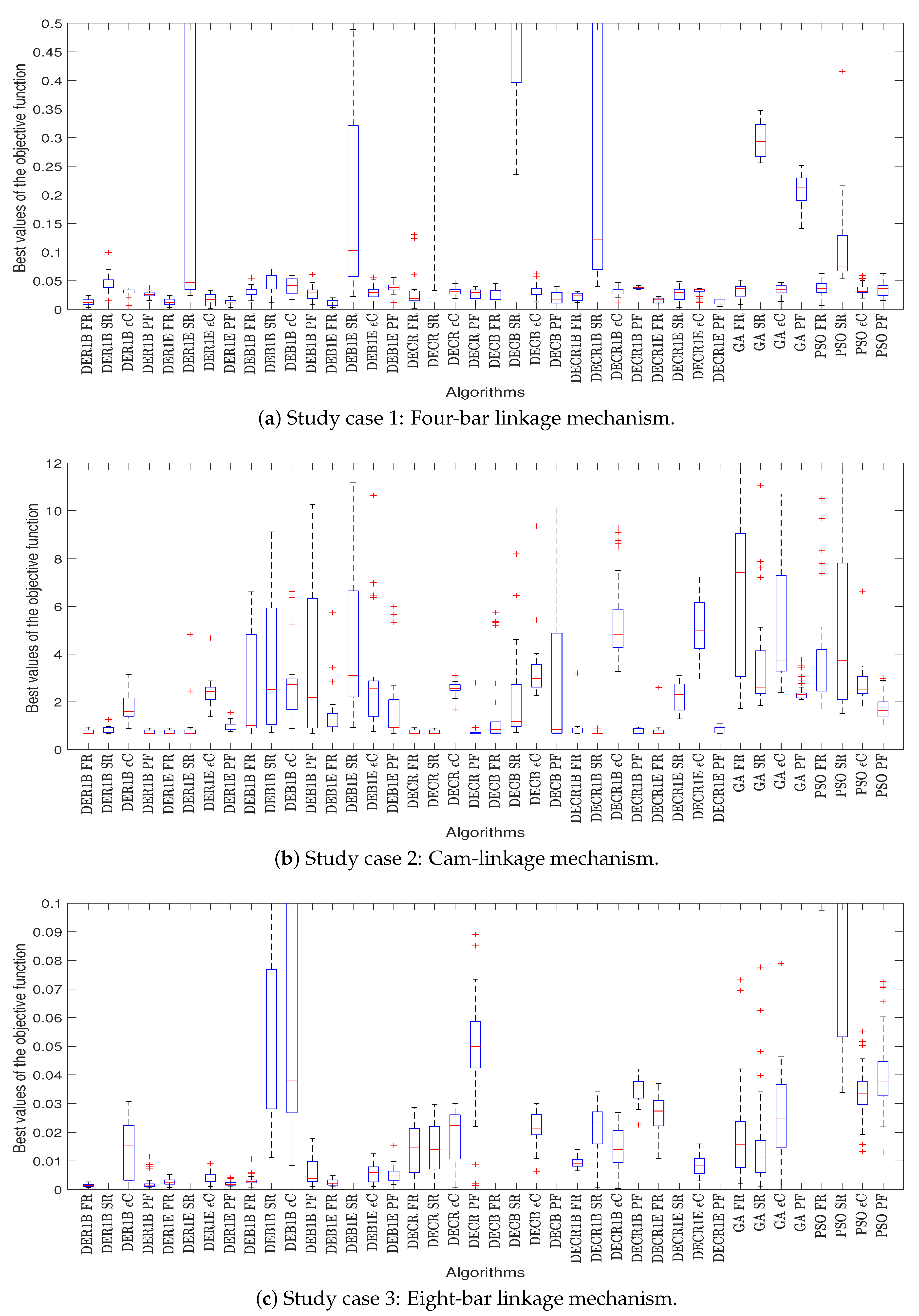The descriptive statistical results are shown in Table A7, Table A8 and Table A9 of Appendix C, and these consider the following measures: the mean, the standard deviation (std), the median, and the maximum (max) and minimum (min) values of the samples. The graphical visualization of the distribution of the samples is shown in the box plot of Figure 5.

Figure 5. Box plot of the sample distribution obtained by the overall performance of the CHTs in ten metaheuristics at each study case of mechanism synthesis for lower limb rehabilitation.

Based on the results presented in such tables, it is possible to define the CHT that delivers the best performance in search of the most promising solution for each study case. Thus, the best behavior of a metaheuristic algorithm is related to the ability to search for the best solutions and provide more reliable results in different runs. The mean, the standard deviation (std), the median, and the maximum (max) and minimum (min) values of the samples are chosen as the statistical measure to indicate the algorithm capacity to find suitable solutions through runs in the particular samples. The best CHT between two CHTs, called A and B, included in the algorithms, is obtained by the following comparison procedure:

• The CHT A can be compared to the CHT B if their CHTs are different, and the algorithms that implement such CHTs are the same. On the contrary, they cannot be compared.
• The statistical measure from the thirty executions of the CHT A is better than the CHT B for the same algorithm if the former presents less value than the latter. When this happens, the CHT A obtains the point (a win) in favor. Thus, the maximum number of points for comparing each CHT is 150 (three CHT comparisons per five measures per ten algorithms).
• The CHT with the highest number of points is the best constraint-handling technique.

In the comparison method, the lower values of the statistical measures (the mean, the standard deviation (std), the median, and the maximum (max) and minimum (min) values of the samples) are preferable in each algorithm. All measures are considered in the comparison procedure. The results obtained by the comparison process are presented in Table 7. The best performances of metaheuristic algorithms include the FR for the solution of the three study cases. For study case 1, it wins 115, for study case 2, it wins 104, and for study case 3, it wins 105. The next CHT alternative is the PF because it obtains the second-best performance in two study cases (study cases 1 and 2).

Table 7. Performance analysis of the CHTs using descriptive statistics.

	Study Case 1				Study Case 2				Study Case 3
	FR	SR	$\mathit{ϵ}$ C	PF	FR	SR	$\mathit{ϵ}$ C	PF	FR	SR	$\mathit{ϵ}$ C	PF
DER1B	14	1	7	8	11	2	3	14	12	0	7	11
DER1E	10	0	7	13	14	7	2	7	11	0	6	13
DEB1B	11	2	5	12	14	2	7	7	15	3	2	10
DEB1E	15	0	8	7	13	0	5	12	15	0	7	8
CR	10	0	8	12	10	15	1	4	11	13	6	0
DECB	11	0	5	14	13	8	1	8	8	5	15	2
DECR1B	14	0	8	8	8	14	0	8	13	5	10	2
DECR1E	11	5	2	12	13	5	0	12	8	1	15	6
GA	11	0	14	5	3	8	6	13	11	13	6	0
PSO	8	0	13	9	5	2	8	15	1	4	14	11
Total	115	8	77	100	104	63	33	100	105	44	88	63

The inferential statistical analysis was performed to make general conclusions about the performance of the CHTs incorporated in the metaheuristic algorithms for the solution of the lower limb rehabilitation mechanism synthesis. Nonparametric statistical tests [61] were used because the independence, normality, and homoscedasticity assumptions in the samples were not fulfilled due to the stochastic nature of the algorithms.

The inferential statistical analysis consists of performing a multi-comparative post-hoc analysis with Holm post-hoc error correction method [61] in all CHTs incorporated in the algorithms. The first step is to guarantee that at least one comparison of the constraint-handling technique in the metaheuristic algorithms is different. The $95\%$-confidence Friedman test is applied for that purpose, and the results are presented in Table A10 of Appendix D. The obtained p-value near to zero proves the existence of such differences with confidence close to $100\%$.

Once the first step was done, the Friedman test for multiple comparisons with the Holm post-hoc error correction method was performed to make the general conclusions of comparisons and confirm the results’ confidence. The forty samples (four CHTs included in ten algorithms), conformed to each one by the best thirty objective functions of the executions, can be compared if both CHTs are incorporated in the same metaheuristic algorithm.

In Table A11 of Appendix D, the results obtained by the multi-comparative analysis are shown. The two-sided alternative hypothesis was selected, which means that, in the case that the p-value of the test is less than the $5\%$ statistical significance, the comparison between the CHT A and the one in B for the same algorithm presents significant differences (the alternative hypothesis is accepted). On the contrary, if the results are not convincing, and significant differences are not observed in the comparative result then the null hypothesis is accepted. Once the alternative hypothesis is accepted, the Friedman z-value sign defines the winner between both CHTs in the algorithms. The negative sign of z indicates that the CHT in the algorithm A was better than the one in B, and vice versa.

Three comparisons related to the four CHTs are made per each metaheuristic algorithm. A total of thirty comparisons are carried out per each CHT at each study case (considering the ten algorithms), and the highest number of wins defines the most suitable constraint-handling technique in the synthesis of lower limb rehabilitation mechanisms for each study case. A total of ninety comparisons was carried out, considering the three CHT comparisons with the ten metaheuristic algorithm for the three study cases.

The number of wins per CHT in algorithms from the comparisons is presented in Table 8. The results indicate that the feasible rules improve the algorithm performance in the comparisons at $66.66\%$ for study case 1, $40\%$ for study case 2, and $53.33\%$ for study case 3. The overall improvement for the ninety comparisons (in all study cases) with the FR is around $53.3\%$. It is also observed in Table A11 of Appendix D that only eight comparisons with other CHTs (DECB EC, DECR1B SR, DECR1E EC, GA SR, GA PF, PSO SR, PSO $ϵ$ C, and PSO PF) outperformed the values obtained in FR (around $8.8\%$ of the total comparisons).

Table 8. The number of wins obtained by each algorithm through Friedman test for multiple comparisons using the execution best values as the sample.

	Study Case 1				Study Case 2				Study Case 3
	FR	SR	$\mathit{ϵ}$ C	PF	FR	SR	$\mathit{ϵ}$ C	PF	FR	SR	$\mathit{ϵ}$ C	PF
DER1B	3	0	1	1	2	1	0	2	2	0	1	2
DER1E	1	0	1	1	2	2	0	1	1	0	1	2
DEB1B	2	0	0	2	0	0	0	0	2	0	0	2
DEB1E	3	0	2	1	2	0	0	2	3	0	1	1
DECR	2	0	1	1	1	1	0	1	1	1	1	0
DECB	1	0	1	2	2	0	0	1	2	0	3	0
DECR1B	3	0	2	1	1	3	0	1	2	1	1	0
DECR1E	2	0	0	2	2	1	0	2	2	0	3	1
GA	2	0	2	1	0	2	1	3	1	1	1	0
PSO	1	0	1	1	0	0	0	3	0	1	2	2
Total	20	0	11	13	12	10	1	16	16	4	14	10

Nevertheless, the obtained solutions in such comparisons did not surpass the best solutions provided by the FR as is observed visually in Figure 5 and numerically in Table A7, Table A8 and Table A9 of Appendix C. Then, the improvement in the eight algorithms using the CHTs in such comparisons did not influence a better overall behavior. In addition, in the remaining ninety comparisons (around $29.44\%$) with respect to the FR, there were no conclusive results about improving an algorithm. The latter means that there are no other CHTs in the algorithms that present a better behavior than the FR.

On the other hand, the penalty function outperformed at $43.33\%$ in study case 1, $53.33\%$ in study case 2, and $33.33\%$ in study case 3 of the comparisons with respect to the other CHTs. The $ϵ$-constraint method improved at $36.66\%$, $3.33\%$, and $46.66\%$ in the corresponding study cases. The stochastic ranking outperformed at $0\%$, $33.33\%$, and $13.33\%$ of the comparisons. Nevertheless, in the last three CHTs, several comparisons exist where the CHTs in the algorithm to which it is compared outperformed such results as shown in Table A11 of Appendix D.

Thus, it is confirmed, with $95\%$ confidence, that the feasibility rules improved the search capabilities of the algorithm with respect to the other CHTs. This implies that the optimal synthesis of the lower limb rehabilitation mechanism can be benefited by using the FR to solve such a constrained optimization problem because this can improve the quality and the consistency of results in most of the algorithms reviewed in this work.

5.3. Statistical Analysis of the CHT Behavior through Metrics

This work is also interested in knowing the search capabilities of metaheuristic algorithms with the constraint-handling techniques related to different performance metrics. Then, six performance metrics [62] found in the specialized literature were used. Each of these metrics is described below:

• The feasibility probability (FP) is obtained by dividing the number of feasible executions by the total number of executions. FP is in the range of $[0,1]$, where 0 represents that there are not feasible solutions, and 1 represents that all found solutions are feasible.
• The convergence probability (P) is obtained by dividing the number of successful executions by the total number of executions. The successful solutions are defined as the solutions x close to the best solution $x^{*}$ in the objective function space. Therefore, a satisfactory solution can be determined by $|\overline{J}\left(x\right)-\overline{J}\left(x^{*}\right)|\le \overline{e}$, where the best executions per each study case is shown in Table A7, Table A8 and Table A9 of Appendix C. The value of $\overline{e}$ is related to the bias region in the synthesis problem where the mechanism executes a suitable rehabilitation routine.
  For the four-bar mechanism, $\overline{J}\left(x^{*}\right)=0.0021$ and $\overline{e}=0.0018$ are considered; for the cam-linkage mechanism, $\overline{J}\left(x^{*}\right)=0.6540$ and $\overline{e}=0.5931$ are chosen; and for the eight-bar linkage mechanism, $\overline{J}\left(x^{*}\right)=1.2054\times {10}^{-4}$ and $\overline{e}=0.0011$ are selected. The P metric value is in the interval $[0,1]$, where a higher value (the best P metric) implies that all executions converge to the region. The metric is related to the reliability of an algorithm to find successful solutions.
• AFES is the average number of function evaluations required for each successful execution. Successful execution is considered when it finds the first solution in the bias region $\overline{e}$. If successful executions are not found, Non-Successful Executions (NSE) are accounted for. The best result in the AFES metric is first related to the minimum value in NSE and then to the lower values of the AFES. This metric indicates a convergence speed measure to the bias region $\overline{e}$.
• Successful performance (SP) divides the AFES by P. The best result in the SP metric is first related to the minimum value in NSE and then to the lower values of the SP.
• EVALS counts the number of evaluations an algorithm needs to find the first feasible solution in every execution. Lower evaluations mean a low computational cost to reach a feasible solution; therefore, this is preferred. This metric is presented with the use of statistics.
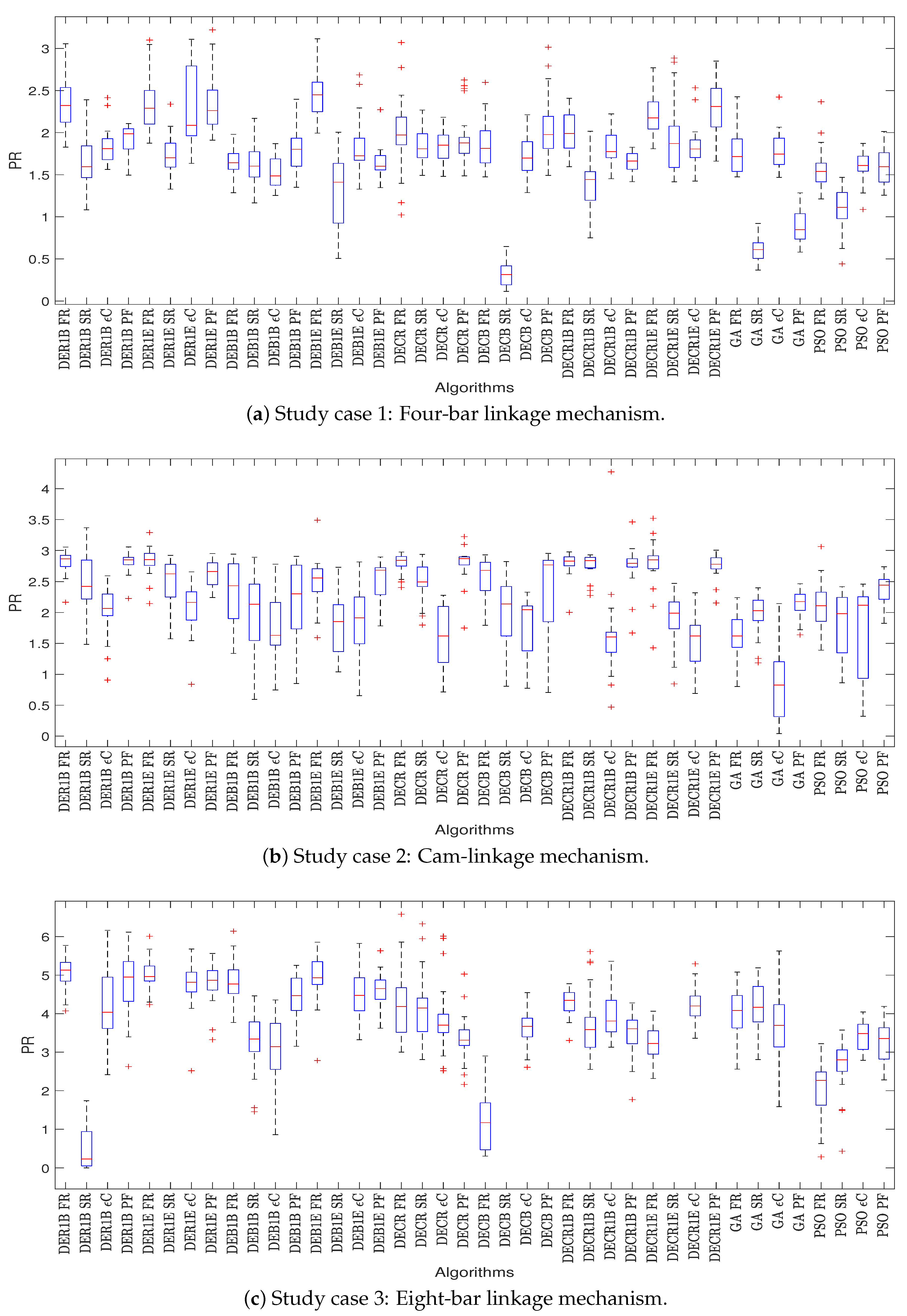
• The Progress Ratio (PR) measures the improvement capability of an algorithm inside the feasible region in every execution. This metric is calculated by (86) where ${\overline{J}}_{min}\left(G_{ff}\right)$ is the value of the objective function of the first feasible solution, and ${\overline{J}}_{min}\left(MCN\right)$ is the value of the objective function of the best feasible solution in the algorithm execution. It is assumed in (86) that ${\overline{J}}_{min}\left(MCN\right)>0$ is fulfilled. A higher value in this metric is preferred and also presented by using statistics.

  $$PR=\left|ln\sqrt{\frac{{\overline{J}}_{min}\left(G_{ff}\right)}{{\overline{J}}_{min}\left(MCN\right)}}\right|$$

  (86)

As commented previously, thirty executions of each constraint-handling technique included in the metaheuristic algorithms were carried out for each study case. The values of the metrics $FP$, P, $AFES$, and $SP$ for the thirty executions for each algorithm at each study case are presented in Table A12, Table A13, Table A14 and Table A15 of Appendix E. The summaries (averages values) of those metrics are displayed in Table 9. We observed that, for the metric FP, the $ϵ$ C provided the best results in the three study cases, followed by the FR and PF, in that order. For the metric P, the FR obtained the best results in cases 1 and 3. In the second study case, the result in FR was close to the best one provided by the PF. In the AFES metric, the FR, $ϵ$ C, and PF won in only one study case. For the SP value, the FR provided the best result in two study cases.

Table 9. Average metric values $FP$, P, $AFES$, and $SP$ for each study case and for each constraint-handling technique included in the metaheuristic algorithms.

CHT	Metric FP				Metric P
	Study Case				Study Case
	1	2	3		1	2	3
FR	$\mathbf{1}$	$\mathbf{1}$	$0.9$		$\mathbf{0}.\mathbf{053}$	$0.7$	$\mathbf{0}.\mathbf{12}$
SR	$0.78$	$0.99$	$0.52$		$0.01$	$0.48$	$0.023$
$ϵC$	$\mathbf{1}$	$\mathbf{1}$	$\mathbf{0}.\mathbf{98}$		$0.04$	$0.08$	$0.047$
PF	$\mathbf{1}$	$\mathbf{1}$	$0.7$		$0.043$	$\mathbf{0}.\mathbf{71}$	$0.09$
CHT	Metric AFES				Metric SP
	Study Case				Study Case
	1	2	3		1	2	3
FR / NSE	$\mathbf{4}.\mathbf{8}\times {\mathbf{10}}^{\mathbf{6}}/\mathbf{5}$	$2.2\times {10}^6/2$	$2.391\times {10}^7/5$		$\mathbf{6}.\mathbf{1}\times {\mathbf{10}}^{\mathbf{7}}/\mathbf{5}$	$2.7\times {10}^6/2$	$\mathbf{1}.\mathbf{3}\times {\mathbf{10}}^{\mathbf{8}}/\mathbf{5}$
SR / NSE	$5.9\times {10}^5/9$	$1.4\times {10}^6/2$	$1.8\times {10}^7/7$		$5.9\times {10}^6/9$	$3\times {10}^6/2$	$3.4\times {10}^8/7$
$ϵC$ / NSE	$4.5\times {10}^6/7$	$1.9\times {10}^5/6$	$\mathbf{2}.\mathbf{386}\times {\mathbf{10}}^{\mathbf{7}}/\mathbf{5}$		$6.7\times {10}^7/7$	$2.1\times {10}^6/6$	$3.4\times {10}^8/5$
PF / NSE	$4.9\times {10}^6/6$	$\mathbf{2}.\mathbf{3}\times {\mathbf{10}}^{\mathbf{6}}/\mathbf{1}$	$2.381\times {10}^7/7$		$4.9\times {10}^7/6$	$\mathbf{3}.\mathbf{5}\times {\mathbf{10}}^{\mathbf{6}}/\mathbf{1}$	$1.3\times {10}^8/7$

In the case of the metrics $EVALS$ and $PR$, inferential statistics using the non-parametric Friedman test for multiple comparisons are included to confirm the performance. The distribution of the samples related to such metric values per each algorithm at each study case is shown in the box plots of Figure 6 and Figure 7, respectively, and the numerical results of the $EVALS$ and $PR$ metrics are presented in Table A16, Table A17, Table A18, Table A21, Table A22 and Table A23 of Appendix E, respectively. The multi comparative Friedman test is presented in Appendix E.6 and Appendix E.8. Summaries of the winning numbers of these comparisons are displayed in Table 10 and Table 11.

Figure 6. Box plot of the sample distribution obtained by EVALS in ten metaheuristics at each study case of mechanism synthesis for lower limb rehabilitation.

Figure 7. Box plot of the sample distribution obtained by PR in ten metaheuristics at each study case of mechanism synthesis for lower limb rehabilitation.

Table 10. Number of winners in the EVALS metric by using the multi comparative test.

	Study Case 1				Study Case 2				Study Case 3
	FR	SR	$\mathit{ϵ}$ C	PF	FR	SR	$\mathit{ϵ}$ C	PF	FR	SR	$\mathit{ϵ}$ C	PF
DER1B	0	0	0	0	2	0	0	0	2	1	0	2
DER1E	0	0	0	0	1	1	0	2	1	0	3	2
DEB1B	0	0	0	0	0	0	0	0	1	3	1	0
DEB1E	0	0	0	0	1	0	0	1	1	0	3	2
DECR	0	0	0	0	2	0	0	1	1	2	2	0
DECB	0	0	0	0	1	0	0	0	2	1	3	0
DECR1B	0	0	0	0	1	1	0	1	1	3	1	0
DECR1E	0	0	0	0	0	0	0	0	2	1	3	0
GA	0	0	0	0	1	1	0	0	1	3	1	0
PSO	0	0	0	0	0	0	0	0	1	3	1	0
Total	0	0	0	0	9	3	0	5	13	17	18	6

Table 11. Number of winners in the PR metric by using the multi comparative test.

	Study Case 1				Study Case 2				Study Case 3
	FR	SR	$\mathit{ϵ}$ C	PF	FR	SR	$\mathit{ϵ}\mathit{C}$	PF	FR	SR	$\mathit{ϵ}\mathit{C}$	PF
DER1B	0	2	1	1	0	1	3	0	1	0	2	1
DER1E	0	3	0	0	0	1	3	1	1	0	1	1
DEB1B	0	1	1	0	0	0	1	0	0	2	2	0
DEB1E	0	2	1	1	0	2	2	0	1	0	1	1
DECR	0	0	0	0	0	2	3	0	0	0	0	3
DECB	0	3	1	0	0	2	2	0	2	1	3	0
DECR1B	0	3	0	2	0	0	3	0	0	1	1	1
DECR1E	0	2	2	0	0	2	2	0	3	1	2	0
GA	0	3	0	2	1	0	3	0	1	1	1	0
PSO	0	3	0	0	1	1	1	0	3	2	0	0
Total	0	22	6	6	2	11	23	1	12	8	13	7

The $EVALS$ metric for study case 1 indicates that feasible solutions were found in the initialization of the 200 individuals (particles) of the population (swarm). As a result, all executions required at least 200 evaluations to find a feasible solution (the feasible region). For this reason, the samples were not significant to determine a winner in the CHT in such a metric. In study case 2, the $FR$ confirmed the superior performance in the $EVALS$ metric. In study case 3, the $ϵ$-constraint method improved the convergence to the feasible region in fewer generations. Finally, in the $PR$ metric, it was confirmed in two study cases that the $ϵ$-constraint method can improve the solutions through the feasible region when the generations occur, followed by the SR that won in only one study case.

According to the results obtained by the previous analysis in the performance metrics, the following findings of the CHTs in the optimal synthesis of the lower limb rehabilitation mechanism synthesis were observed:

• The FR had one of the best performance and the best one of the search for feasible solutions and satisfactory regions for the three study cases, respectively, because this constraint-handling technique has a high probability value in the FP and P metrics. The relationship between the AFES and P gave by SP is the best among the CHTs. Therefore, among the studied CHTs, the Feasibility Rules technique is the most reliable one for the synthesis of mechanisms for rehabilitation.
• The PF can be considered the second option for solving mechanism synthesis for rehabilitation problems because it showed a suitable performance to find satisfactory solutions (P and SP metrics) compared to Stochastic-Ranking and $ϵ$-constraint. This establishes acceptable reliability to find feasible solutions (FP metric).
• $ϵ$ C method presented the best performance in the search for feasible regions as shown in FP. Inside the feasible region, this CHT produces improved solutions based on the PR metric. Nevertheless, the probability of this CHT to search for satisfactory solutions was low (P and SP metrics). This behavior is attributed to the gradient-based mutation where fast convergence to feasible local regions is promoted.
• SR is the less reliable CHT because some algorithm executions can not find feasible solutions (FP metric). This presents a low performance in the search for suitable solutions (P metric).

According to the results in this section, the Feasibility Rules presented the best performance for handling constraints in the mechanism synthesis for rehabilitation problems. The Penalty Functions gave the second best performance. Those CHTs improved the quality and the consistency in most of the algorithms reviewed in this work.

5.4. Evaluation of the Obtained Mechanisms

In this section, the best solutions obtained by the feasibility rules (according to the overall performance presented in Table 8), and the worst constraint-handling technique are presented.

In study case 1, the best constraint-handling technique was the feasibility rules, and the worst was stochastic-ranking. The Computer-Aided Design (CAD) and the generated trajectory of the best mechanisms obtained by both constraint-handling techniques are presented in Figure 8, where the objective function values of the mechanisms obtained by the feasibility rules (with the algorithm DECR) is $J=0.002098$, and by stochastic-ranking (with the algorithm DECR1E) is $J=0.003726$. Those values are given in Table A7 of Appendix C.

Figure 8. CAD representation and trajectory generated of the mechanisms (design goals) given by the best and the worst constraint-handling technique for solving study case 1.

According to the design parameters obtained in both CHTs (see Table A26 of Appendix F), the feasibility rules present a Pearson correlation coefficient of $0.9939$ with respect to the stochastic-ranking. This indicates a high degree of similarity (see Figure 8). On the other hand, the performance of the design goals is presented in Figure 8c,d. Figure 8c shows the trajectory of the mechanisms, the current, and the desired precision points. The average error between the desired precision points and the current ones is $\overline{J_1}=4.7095\times {10}^{-4}$ [m] by Feasibility Rules (FR) and $\overline{J_1}=4.6009\times {10}^{-4}$ [m] by Stochastic-Ranking (SR).

Figure 8d shows the angles obtained by the crank and the desired angles, where the average angular error is $\overline{J_2}=1.6270$ [rad] by feasibility rules, and $\overline{J_2}=3.2663$ [rad] by stochastic-ranking. We observed that the design goals in both mechanisms related to $\overline{J_1}$ and $J_2$, present a trade-off, i.e., in one goal, it is better but in the other not. Then, solutions obtained by the feasible rules and the stochastic-ranking are suitable for the rehabilitation mechanism. Nevertheless, the feasible rules provide more reliable results through different algorithm executions and with a better overall performance (related to the objective function J).

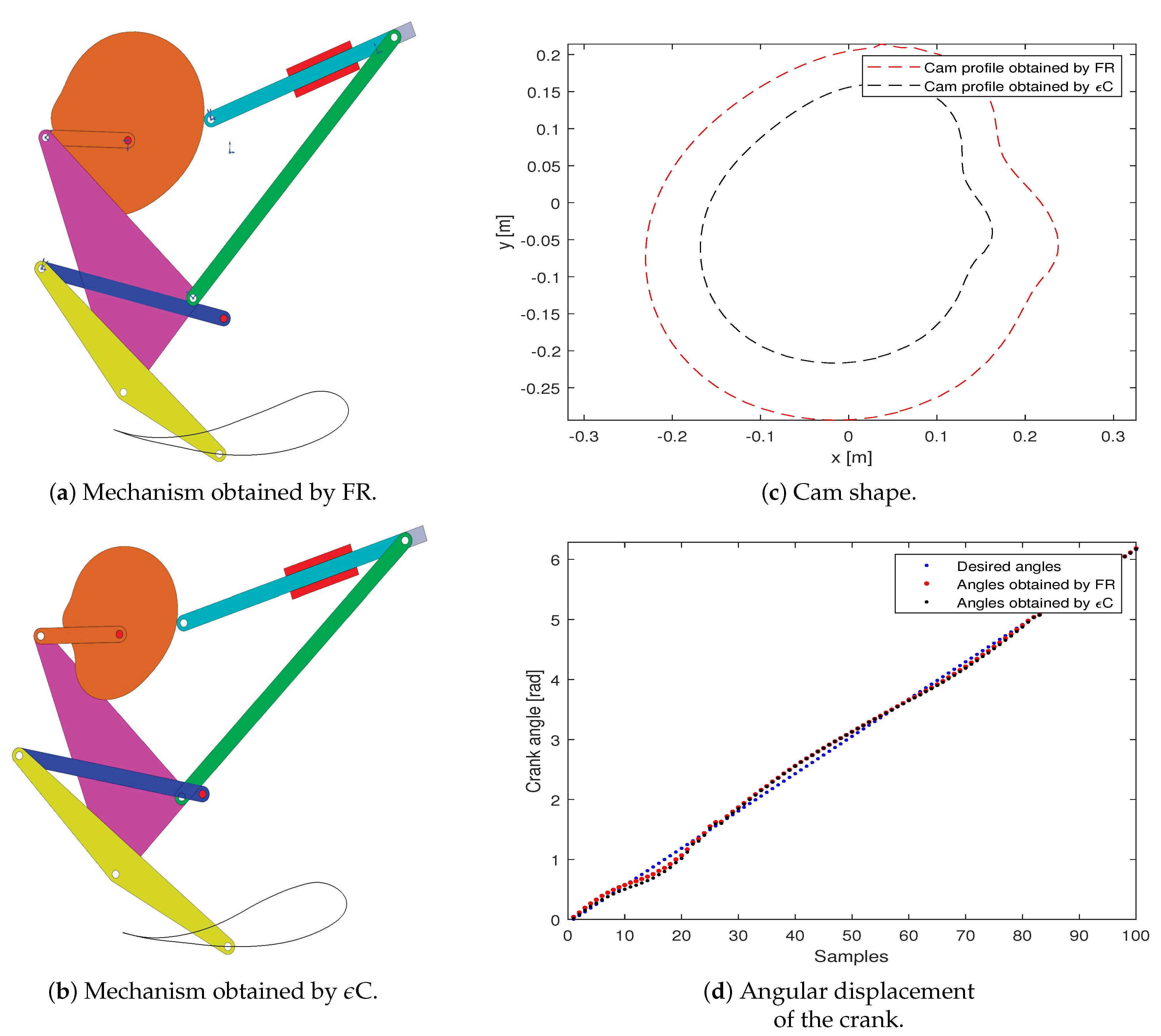
In study case 2, the feasibility rule was the best constraint-handling technique, and the worst was the epsilon-constraint. The CAD and the generated trajectory of the best mechanisms obtained by both constraint-handling techniques are presented in Figure 9. The objective function values given by the mechanisms obtained by the feasibility rules (DEB1B) is $J=0.6557$ and by epsilon-constraint (DEB1E) is $J=0.7588$. Those values are given in Table A8 of Appendix C.

Figure 9. CAD representation and design goals of the mechanism (related to the terms $\overline{J_1}$ and ${\overline{J}}_2$) given by the best and the worst constraint-handling technique for solving study case 2.

According to the design parameters obtained in both CHTs (see Table A27 of Appendix F), the feasibility rules present a Pearson correlation coefficient of $0.9991$ with respect to the epsilon-constraint. This correlation is larger than the obtained mechanisms in the previous study case 1, which implies a fairly strong relationship. In order to highlight the difference, the performance of the design goals is presented in Figure 9c,d for the cam shapes and the angles obtained by the crank, respectively.

The normalized average error between the desired crank angles and the current ones is $\overline{J_1}=1.2217$ by feasibility rules and $\overline{J_1}=1.7122$ by epsilon-constraint. The normalized base radius of the cam is $\overline{J_2}=0.4137$ by FR, and $\overline{J_2}=0.3502$ by epsilon-constraint. It is observed again that the design goals present a trade-off, such that both mechanisms are suitable for the rehabilitation routine, and it depends on the application that one selects. However, the feasible rules can search for solutions with a similar performance through different executions and with better quality in the overall performance in the weighted objective function J.

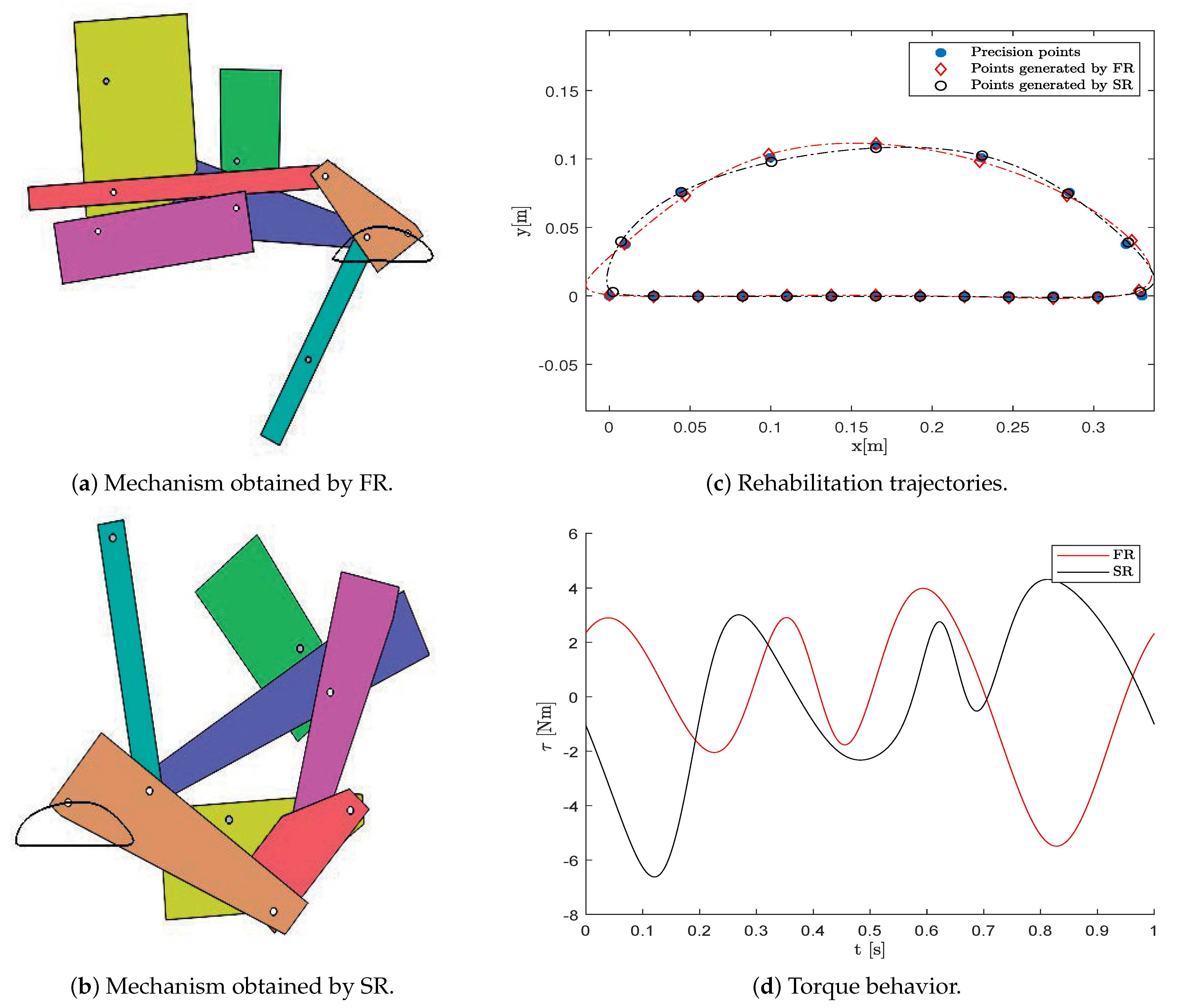
Finally, for study case 3, the best constraint-handling technique was the feasibility rules, and the worst one was stochastic-ranking. The CAD and the generated trajectory are presented in Figure 10, where the objective function values of the mechanisms obtained by the feasibility rules (DECR) is $J=0.0001903$, and by stochastic-ranking (DECR) is $J=0.0001884$. Those values are given in Table A9 of Appendix C.

Figure 10. CAD representation and trajectory generated of the mechanism (related to the design goals) given by the best and the worst constraint-handling technique for solving study case 3.

According to the design parameters obtained in both CHTs (see Table A28 of Appendix F), the feasibility rules present a Pearson correlation coefficient of $0.7231$ with respect to the stochastic-ranking. As the problem complexity in study case 3 is higher than in the other cases, the obtained solution presents differences, as is observed in Figure 10a,b. The behavior of the design goals related to the generated trajectory in the mechanisms and the torque applied in the crank link are displayed in Figure 10c,d, respectively.

In this case, the average error between the desired precision points and the current ones is $\overline{J_1}=8.1216\times {10}^{-5}$ [m] by feasibility rules and $\overline{J_1}=5.9633\times {10}^{-5}$ [m] by stochastic-ranking. The average torque is $\overline{J_2}=5.4531$ [Nm] by feasibility rules, and $\overline{J_2}=6.4395$ [Nm] by stochastic-ranking. Neither mechanism can be considered the best because they present a trade-off in the design goals. Thus, design solutions obtained by the feasible rules and the stochastic-ranking are suitable for the rehabilitation mechanism. Nevertheless, the feasible rule provides more reliable results through different executions and the second-best overall performance (related to the objective function J).

6. Conclusions

In this work, the behavior of four constraint-handling techniques for the synthesis of rehabilitation mechanisms is studied in ten metaheuristic algorithms.

According to the results, we present the following conclusions:

• Through the statistical analysis, we observed that the feasibility rules present the best overall performance for the solution of the three mechanism synthesis cases under study. This is because the feasibility rules show a high probability of convergence towards feasible solutions and satisfactory regions based on the performance metrics studied in this work.
• In the solution of mechanism synthesis problems for rehabilitation, there exists a high probability that the search capability of an algorithm is improved by incorporating the FR because, in most of the algorithms reviewed in this work, the FR enhanced the quality and consistency of results.
• The penalty functions can be used as the second option for solving mechanism synthesis for rehabilitation problems. These establish acceptable reliability to find feasible solutions based on the performance metrics.
• The $ϵ$-constraint method and stochastic-ranking presented the worst overall performance in the solution of the mechanism synthesis for lower limb rehabilitation. This feature is due to the mechanism synthesis problem, which presents a complex search space and wide, with highly nonlinear functions (multimodality), several design variables, and feasible regions that are difficult to find. The $ϵ$-constraint presents a fast convergence to feasible local regions because the gradient-based mutation increases the speed in the search of feasible solutions.
• We confirmed that all study cases for the assessment of the obtained mechanisms, by using the feasibility rules and the worst CHT, presented different trade-offs in the design goals of the mechanism synthesis problem for lower limb rehabilitation. Nevertheless, FR can endow the algorithm with a better search capability to find reliable results through different executions with a high probability of finding the best overall performance.

Appendix A.1. Precision Points for the Case 1: Four-Bar Linkage Mechanism

For the synthesis of the four-bar mechanism, the standard path of the ankle of a 12-year-old child is considered. In Table A1, those data are shown and are obtained by [16].

Table A1. Precision points for study case 1: Four-bar linkage mechanism.

i	${\overline{\mathit{x}}}_{\mathit{P}}^{\mathit{i}}$ [m]	${\overline{\mathit{y}}}_{\mathit{P}}^{\mathit{i}}$ [m]
1	0.7429	0.1880
2	0.6551	0.1573
3	0.6014	0.1388
4	0.5189	0.1149
5	0.4159	0.1012
6	0.3001	0.1074
7	0.1964	0.1375
8	0.1639	0.1662
9	0.1605	0.2003
10	0.1934	0.2256
11	0.2619	0.2251
12	0.4201	0.1808
13	0.6474	0.1607
14	0.7429	0.1880

Table A1. Precision points for study case 1: Four-bar linkage mechanism.

i	${\overline{\mathit{x}}}_{\mathit{P}}^{\mathit{i}}$ [m]	${\overline{\mathit{y}}}_{\mathit{P}}^{\mathit{i}}$ [m]
1	0.7429	0.1880
2	0.6551	0.1573
3	0.6014	0.1388
4	0.5189	0.1149
5	0.4159	0.1012
6	0.3001	0.1074
7	0.1964	0.1375
8	0.1639	0.1662
9	0.1605	0.2003
10	0.1934	0.2256
11	0.2619	0.2251
12	0.4201	0.1808
13	0.6474	0.1607
14	0.7429	0.1880

Appendix A.2. Precision Points for Case 2: Cam-Linkage Mechanism

For the synthesis of the cam-linkage mechanism, the data in Table A2 are considered. These data represent the ankle path in the standard gait for an adult with a thigh-length $L_{thigh}=0.3984$ [m] and a shank-length of $L_{shank}=0.3956$ [m].

Table A2. Precision points for study case 2: Cam-linkage mechanism.

i	${\overline{\mathit{x}}}_{\mathit{P}}^{\mathit{i}}$ [m]	${\overline{\mathit{y}}}_{\mathit{P}}^{\mathit{i}}$ [m]	i	${\overline{\mathit{x}}}_{\mathit{P}}^{\mathit{i}}$ [m]	${\overline{\mathit{y}}}_{\mathit{P}}^{\mathit{i}}$ [m]	i	${\overline{\mathit{x}}}_{\mathit{P}}^{\mathit{i}}$ [m]	${\overline{\mathit{y}}}_{\mathit{P}}^{\mathit{i}}$ [m]
1	−0.3159	−0.7259	2	−0.3054	−0.7295	3	−0.2956	−0.7326	4	−0.2850	−0.7357
5	−0.2730	−0.7388	6	−0.2596	−0.7421	7	−0.2455	−0.7453	8	−0.2307	−0.7484
9	−0.2172	−0.7509	10	−0.2019	−0.7540	11	−0.1885	−0.7567	12	−0.1738	−0.7596
13	−0.1612	−0.7623	14	−0.1479	−0.7650	15	−0.1345	−0.7677	16	−0.1225	−0.7703
17	−0.1112	−0.7726	18	−0.0984	−0.7750	19	−0.0870	−0.7772	20	−0.0748	−0.7792
21	−0.0633	−0.7810	22	−0.0517	−0.7826	23	−0.0401	−0.7840	24	−0.0285	−0.7853
25	−0.0162	−0.7862	26	−0.0045	−0.7870	27	0.0079	−0.7875	28	0.0196	−0.7879
29	0.0306	−0.7881	30	0.0431	−0.7880	31	0.0548	−0.7876	32	0.0672	−0.7871
33	0.0789	−0.7863	34	0.0913	−0.7853	35	0.1023	−0.7842	36	0.1139	−0.7827
37	0.1262	−0.7810	38	0.1378	−0.7791	39	0.1500	−0.7768	40	0.1622	−0.7743
41	0.1757	−0.7713	42	0.1884	−0.7681	43	0.2017	−0.7644	44	0.2143	−0.7607
45	0.2280	−0.7562	46	0.2403	−0.7518	47	0.2538	−0.7466	48	0.2652	−0.7418
49	0.2777	−0.7360	50	0.2894	−0.7301	51	0.3008	−0.7238	52	0.3107	−0.7174
53	0.3203	−0.7106	54	0.3282	−0.7037	55	0.3352	−0.6964	56	0.3400	−0.6894
57	0.3436	−0.6819	58	0.3456	−0.6743	59	0.3465	−0.6662	60	0.3442	−0.6590
61	0.3408	−0.6514	62	0.3356	−0.6443	63	0.3279	−0.6379	64	0.3185	−0.6320
65	0.3075	−0.6279	66	0.2956	−0.6243	67	0.2810	−0.6230	68	0.2664	−0.6224
69	0.2499	−0.6241	70	0.2322	−0.6269	71	0.2145	−0.6312	72	0.1955	−0.6366
73	0.1756	−0.6431	74	0.1540	−0.6505	75	0.1330	−0.6582	76	0.1107	−0.6668
77	0.0880	−0.6752	78	0.0627	−0.6844	79	0.0380	−0.6931	80	0.0140	−0.7012
81	−0.0130	−0.7095	82	−0.0388	−0.7168	83	−0.0657	−0.7235	84	−0.0932	−0.7292
85	−0.1199	−0.7340	86	−0.1476	−0.7372	87	−0.1723	−0.7397	88	−0.1978	−0.7406
89	−0.2227	−0.7402	90	−0.2449	−0.7388	91	−0.2669	−0.7360	92	−0.2841	−0.7333
93	−0.2996	−0.7298	94	−0.3130	−0.7261	95	−0.3217	−0.7237	96	−0.3288	−0.7212
97	−0.3321	−0.7200	98	−0.3322	−0.7202	99	−0.3296	−0.7213	100	−0.3232	−0.7238
101	−0.3167	−0.7262

Table A2. Precision points for study case 2: Cam-linkage mechanism.

i	${\overline{\mathit{x}}}_{\mathit{P}}^{\mathit{i}}$ [m]	${\overline{\mathit{y}}}_{\mathit{P}}^{\mathit{i}}$ [m]	i	${\overline{\mathit{x}}}_{\mathit{P}}^{\mathit{i}}$ [m]	${\overline{\mathit{y}}}_{\mathit{P}}^{\mathit{i}}$ [m]	i	${\overline{\mathit{x}}}_{\mathit{P}}^{\mathit{i}}$ [m]	${\overline{\mathit{y}}}_{\mathit{P}}^{\mathit{i}}$ [m]
1	−0.3159	−0.7259	2	−0.3054	−0.7295	3	−0.2956	−0.7326	4	−0.2850	−0.7357
5	−0.2730	−0.7388	6	−0.2596	−0.7421	7	−0.2455	−0.7453	8	−0.2307	−0.7484
9	−0.2172	−0.7509	10	−0.2019	−0.7540	11	−0.1885	−0.7567	12	−0.1738	−0.7596
13	−0.1612	−0.7623	14	−0.1479	−0.7650	15	−0.1345	−0.7677	16	−0.1225	−0.7703
17	−0.1112	−0.7726	18	−0.0984	−0.7750	19	−0.0870	−0.7772	20	−0.0748	−0.7792
21	−0.0633	−0.7810	22	−0.0517	−0.7826	23	−0.0401	−0.7840	24	−0.0285	−0.7853
25	−0.0162	−0.7862	26	−0.0045	−0.7870	27	0.0079	−0.7875	28	0.0196	−0.7879
29	0.0306	−0.7881	30	0.0431	−0.7880	31	0.0548	−0.7876	32	0.0672	−0.7871
33	0.0789	−0.7863	34	0.0913	−0.7853	35	0.1023	−0.7842	36	0.1139	−0.7827
37	0.1262	−0.7810	38	0.1378	−0.7791	39	0.1500	−0.7768	40	0.1622	−0.7743
41	0.1757	−0.7713	42	0.1884	−0.7681	43	0.2017	−0.7644	44	0.2143	−0.7607
45	0.2280	−0.7562	46	0.2403	−0.7518	47	0.2538	−0.7466	48	0.2652	−0.7418
49	0.2777	−0.7360	50	0.2894	−0.7301	51	0.3008	−0.7238	52	0.3107	−0.7174
53	0.3203	−0.7106	54	0.3282	−0.7037	55	0.3352	−0.6964	56	0.3400	−0.6894
57	0.3436	−0.6819	58	0.3456	−0.6743	59	0.3465	−0.6662	60	0.3442	−0.6590
61	0.3408	−0.6514	62	0.3356	−0.6443	63	0.3279	−0.6379	64	0.3185	−0.6320
65	0.3075	−0.6279	66	0.2956	−0.6243	67	0.2810	−0.6230	68	0.2664	−0.6224
69	0.2499	−0.6241	70	0.2322	−0.6269	71	0.2145	−0.6312	72	0.1955	−0.6366
73	0.1756	−0.6431	74	0.1540	−0.6505	75	0.1330	−0.6582	76	0.1107	−0.6668
77	0.0880	−0.6752	78	0.0627	−0.6844	79	0.0380	−0.6931	80	0.0140	−0.7012
81	−0.0130	−0.7095	82	−0.0388	−0.7168	83	−0.0657	−0.7235	84	−0.0932	−0.7292
85	−0.1199	−0.7340	86	−0.1476	−0.7372	87	−0.1723	−0.7397	88	−0.1978	−0.7406
89	−0.2227	−0.7402	90	−0.2449	−0.7388	91	−0.2669	−0.7360	92	−0.2841	−0.7333
93	−0.2996	−0.7298	94	−0.3130	−0.7261	95	−0.3217	−0.7237	96	−0.3288	−0.7212
97	−0.3321	−0.7200	98	−0.3322	−0.7202	99	−0.3296	−0.7213	100	−0.3232	−0.7238
101	−0.3167	−0.7262

Appendix B.1. Parameter Tuning of the Case 1: Four-Bar Linkage Mechanism

The parameters obtained by the irace program for the four-bar mechanism are presented in Table A4.

Table A4. Tuned parameters by irace program for study case 1: Four-bar linkage mechanism.

Algorithm	CHT	Parameters
DER1B	DEB	$CR=0.95$, $F_{min}=0.13$, $F_{max}=0.95$
	SR	$CR=0.91$, $F_{min}=0.23$, $F_{max}=0.96$, $Pf=0.15$
	$ϵ$ C	$CR=0.89$, $F_{min}=0.20$, $F_{max}=0.81$, $Pg=0.07$, $Tc=590$, $Rg=5$, $cp=6$
	PF	$CR=0.95$, $F_{min}=0.17$, $F_{max}=0.91$
DER1E	DEB	$CR=0.99$, $F_{min}=0.23$, $F_{max}=0.86$
	SR	$CR=0.96$, $F_{min}=0.47$, $F_{max}=0.90$, $Pf=0.05$
	$ϵ$ C	$CR=0.88$, $F_{min}=0.14$, $F_{max}=0.87$, $Pg=0.03$, $Tc=430$, $Rg=3$, $cp=10$
	PF	$CR=0.97$, $F_{min}=0.06$, $F_{max}=0.95$
DEB1B	DEB	$CR=0.76$, $F_{min}=0.50$, $F_{max}=0.66$
	SR	$CR=0.97$, $F_{min}=0.23$, $F_{max}=0.97$, $Pf=0.18$
	$ϵ$ C	$CR=0.83$, $F_{min}=0.50$, $F_{max}=0.50$, $Pg=0.08$, $Tc=490$, $Rg=3$, $cp=6$
	PF	$CR=0.67$, $F_{min}=0.59$, $F_{max}=0.61$
DEB1E	DEB	$CR=0.89$, $F_{min}=0.48$, $F_{max}=0.77$
	SR	$CR=0.91$, $F_{min}=0.57$, $F_{max}=0.74$, $Pf=0.30$
	$ϵ$ C	$CR=0.95$, $F_{min}=0.32$, $F_{max}=0.85$, $Pg=0.09$, $Tc=400$, $Rg=3$, $cp=5$
	PF	$CR=0.91$, $F_{min}=0.52$, $F_{max}=0.77$
DECR	DEB	$F_{min}=0.26$, $F_{max}=0.98$, $K_{min}=0.91$, $K_{max}=0.99$
	SR	$F_{min}=0.48$, $F_{max}=0.79$, $K_{min}=0.13$, $K_{max}=0.87$, $Pf=0.42$
	$ϵ$ C	$F_{min}=0.15$, $F_{max}=0.89$, $K_{min}=0.82$, $K_{max}=0.96$, $Pg=0.10$, $Tc=550$, $Rg=5$, $cp=3$
	PF	$F_{min}=0.23$, $F_{max}=0.93$, $K_{min}=0.88$, $K_{max}=0.98$
DECB	DEB	$F_{min}=0.44$, $F_{max}=0.97$, $K_{min}=0.48$, $K_{max}=1$
	SR	$F_{min}=0.29$, $F_{max}=0.91$, $K_{min}=0.29$, $K_{max}=0.69$, $Pf=0.40$
	$ϵ$ C	$F_{min}=0.36$, $F_{max}=0.75$, $K_{min}=0.20$, $K_{max}=0.85$, $Pg=0.05$, $Tc=430$, $Rg=5$, $cp=10$
	PF	$F_{min}=0.53$, $F_{max}=0.89$, $K_{min}=0.34$, $K_{max}=0.98$
DECR1B	DEB	$CR=0.92$, $F_{min}=0.41$, $F_{max}=0.76$, $K_{min}=0.95$, $K_{max}=0.95$
	SR	$CR=0.96$, $F_{min}=0.46$, $F_{max}=0.89$, $K_{min}=0.46$, $K_{max}=0.72$, $Pf=0.12$
	$ϵ$ C	$CR=0.97$, $F_{min}=0.11$, $F_{max}=0.99$, $K_{min}=0.56$, $K_{max}=0.56$, $Pg=0.08$, $Tc=700$, $Rg=2$, $cp=7$
	PF	$CR=0.92$, $F_{min}=0.33$, $F_{max}=0.84$, $K_{min}=0.96$, $K_{max}=0.97$
DECR1E	DEB	$CR=0.92$, $F_{min}=0.32$, $F_{max}=0.72$, $K_{min}=0.29$, $K_{max}=0.77$
	SR	$CR=0.95$, $F_{min}=0.06$, $F_{max}=0.99$, $K_{min}=0.08$, $K_{max}=0.26$, $Pf=0.01$
	$ϵ$ C	$CR=0.96$, $F_{min}=0.08$, $F_{max}=0.94$, $K_{min}=0.42$, $K_{max}=0.87$, $Pg=0.06$, $Tc=740$, $Rg=3$, $cp=9$
	PF	$CR=0.39$, $F_{min}=0.44$, $F_{max}=0.51$, $K_{min}=0.46$, $K_{max}=0.65$
GA	DEB	$CR=0.80$, $MR=0.06$
	SR	$CR=0.23$, $Pf=0.20$, $MR=0.05$
	$ϵ$ C	$CR=1$, $Pg=0.05$, $Tc=610$, $Rg=4$, $cp=8$, $MR=0.08$
	PF	$CR=0.83$, $MR=0.11$
PSO	DEB	$v_{max}=0.01$, $C1=1.29$, $C2=2.04$
	SR	$Pf=0.69$, $v_{max}=0.01$, $C1=2.22$, $C2=1.06$
	$ϵ$ C	$Pg=0.05$, $Tc=610$, $Rg=4$, $cp=8$, $v_{max}=0.01$, $C1=1.10$, $C2=1.79$
	PF	$v_{min}=0.05$, $v_{max}=0.17$, $C1=2.04$, $C2=1.06$

Table A4. Tuned parameters by irace program for study case 1: Four-bar linkage mechanism.

Algorithm	CHT	Parameters
DER1B	DEB	$CR=0.95$, $F_{min}=0.13$, $F_{max}=0.95$
	SR	$CR=0.91$, $F_{min}=0.23$, $F_{max}=0.96$, $Pf=0.15$
	$ϵ$ C	$CR=0.89$, $F_{min}=0.20$, $F_{max}=0.81$, $Pg=0.07$, $Tc=590$, $Rg=5$, $cp=6$
	PF	$CR=0.95$, $F_{min}=0.17$, $F_{max}=0.91$
DER1E	DEB	$CR=0.99$, $F_{min}=0.23$, $F_{max}=0.86$
	SR	$CR=0.96$, $F_{min}=0.47$, $F_{max}=0.90$, $Pf=0.05$
	$ϵ$ C	$CR=0.88$, $F_{min}=0.14$, $F_{max}=0.87$, $Pg=0.03$, $Tc=430$, $Rg=3$, $cp=10$
	PF	$CR=0.97$, $F_{min}=0.06$, $F_{max}=0.95$
DEB1B	DEB	$CR=0.76$, $F_{min}=0.50$, $F_{max}=0.66$
	SR	$CR=0.97$, $F_{min}=0.23$, $F_{max}=0.97$, $Pf=0.18$
	$ϵ$ C	$CR=0.83$, $F_{min}=0.50$, $F_{max}=0.50$, $Pg=0.08$, $Tc=490$, $Rg=3$, $cp=6$
	PF	$CR=0.67$, $F_{min}=0.59$, $F_{max}=0.61$
DEB1E	DEB	$CR=0.89$, $F_{min}=0.48$, $F_{max}=0.77$
	SR	$CR=0.91$, $F_{min}=0.57$, $F_{max}=0.74$, $Pf=0.30$
	$ϵ$ C	$CR=0.95$, $F_{min}=0.32$, $F_{max}=0.85$, $Pg=0.09$, $Tc=400$, $Rg=3$, $cp=5$
	PF	$CR=0.91$, $F_{min}=0.52$, $F_{max}=0.77$
DECR	DEB	$F_{min}=0.26$, $F_{max}=0.98$, $K_{min}=0.91$, $K_{max}=0.99$
	SR	$F_{min}=0.48$, $F_{max}=0.79$, $K_{min}=0.13$, $K_{max}=0.87$, $Pf=0.42$
	$ϵ$ C	$F_{min}=0.15$, $F_{max}=0.89$, $K_{min}=0.82$, $K_{max}=0.96$, $Pg=0.10$, $Tc=550$, $Rg=5$, $cp=3$
	PF	$F_{min}=0.23$, $F_{max}=0.93$, $K_{min}=0.88$, $K_{max}=0.98$
DECB	DEB	$F_{min}=0.44$, $F_{max}=0.97$, $K_{min}=0.48$, $K_{max}=1$
	SR	$F_{min}=0.29$, $F_{max}=0.91$, $K_{min}=0.29$, $K_{max}=0.69$, $Pf=0.40$
	$ϵ$ C	$F_{min}=0.36$, $F_{max}=0.75$, $K_{min}=0.20$, $K_{max}=0.85$, $Pg=0.05$, $Tc=430$, $Rg=5$, $cp=10$
	PF	$F_{min}=0.53$, $F_{max}=0.89$, $K_{min}=0.34$, $K_{max}=0.98$
DECR1B	DEB	$CR=0.92$, $F_{min}=0.41$, $F_{max}=0.76$, $K_{min}=0.95$, $K_{max}=0.95$
	SR	$CR=0.96$, $F_{min}=0.46$, $F_{max}=0.89$, $K_{min}=0.46$, $K_{max}=0.72$, $Pf=0.12$
	$ϵ$ C	$CR=0.97$, $F_{min}=0.11$, $F_{max}=0.99$, $K_{min}=0.56$, $K_{max}=0.56$, $Pg=0.08$, $Tc=700$, $Rg=2$, $cp=7$
	PF	$CR=0.92$, $F_{min}=0.33$, $F_{max}=0.84$, $K_{min}=0.96$, $K_{max}=0.97$
DECR1E	DEB	$CR=0.92$, $F_{min}=0.32$, $F_{max}=0.72$, $K_{min}=0.29$, $K_{max}=0.77$
	SR	$CR=0.95$, $F_{min}=0.06$, $F_{max}=0.99$, $K_{min}=0.08$, $K_{max}=0.26$, $Pf=0.01$
	$ϵ$ C	$CR=0.96$, $F_{min}=0.08$, $F_{max}=0.94$, $K_{min}=0.42$, $K_{max}=0.87$, $Pg=0.06$, $Tc=740$, $Rg=3$, $cp=9$
	PF	$CR=0.39$, $F_{min}=0.44$, $F_{max}=0.51$, $K_{min}=0.46$, $K_{max}=0.65$
GA	DEB	$CR=0.80$, $MR=0.06$
	SR	$CR=0.23$, $Pf=0.20$, $MR=0.05$
	$ϵ$ C	$CR=1$, $Pg=0.05$, $Tc=610$, $Rg=4$, $cp=8$, $MR=0.08$
	PF	$CR=0.83$, $MR=0.11$
PSO	DEB	$v_{max}=0.01$, $C1=1.29$, $C2=2.04$
	SR	$Pf=0.69$, $v_{max}=0.01$, $C1=2.22$, $C2=1.06$
	$ϵ$ C	$Pg=0.05$, $Tc=610$, $Rg=4$, $cp=8$, $v_{max}=0.01$, $C1=1.10$, $C2=1.79$
	PF	$v_{min}=0.05$, $v_{max}=0.17$, $C1=2.04$, $C2=1.06$

Appendix B.2. Parameter Tuning of Case 2: Cam-Linkage Mechanism

The parameters obtained by the irace program for study case 2 related to the cam-linkage mechanism are stated in Table A5.

Table A5. Tuned parameters by irace program for the study case 2: Cam-linkage mechanism.

Algorithm	CHT	Parameters
DER1B	DEB	$CR=0.87$, $F_{min}=0.51$, $F_{max}=0.53$
	SR	$CR=0.91$, $F_{min}=0.46$, $F_{max}=0.70$, $Pf=0.52$
	$ϵ$ C	$CR=0.92$, $F_{min}=0.53$, $F_{max}=0.56$, $Pg=0.04$, $Tc=430$, $Rg=5$, $cp=9$
	PF	$CR=0.93$, $F_{min}=0.52$, $F_{max}=0.63$
DER1E	DEB	$CR=0.94$, $F_{min}=0.47$, $F_{max}=0.58$
	SR	$CR=0.98$, $F_{min}=0.56$, $F_{max}=0.75$, $Pf=0.50$
	$ϵ$ C	$CR=0.99$, $F_{min}=0.51$, $F_{max}=0.66$, $Pg=0.09$, $Tc=230$, $Rg=5$, $cp=6$
	PF	$CR=0.88$, $F_{min}=0.25$, $F_{max}=0.43$
DEB1B	DEB	$CR=0.88$, $F_{min}=0.80$, $F_{max}=0.87$
	SR	$CR=0.99$, $F_{min}=0.62$, $F_{max}=0.75$, $Pf=0.49$
	$ϵ$ C	$CR=0.92$, $F_{min}=0.59$, $F_{max}=0.61$, $Pg=0.05$, $Tc=380$, $Rg=2$, $cp=8$
	PF	$CR=0.90$, $F_{min}=0.63$, $F_{max}=0.87$
DEB1E	DEB	$CR=0.83$, $F_{min}=0.11$, $F_{max}=0.98$
	SR	$CR=0.95$, $F_{min}=0.65$, $F_{max}=0.70$, $Pf=0.50$
	$ϵ$ C	$CR=0.92$, $F_{min}=0.55$, $F_{max}=0.61$, $Pg=0.06$, $Tc=370$, $Rg=2$, $cp=8$
	PF	$CR=0.92$, $F_{min}=0.65$, $F_{max}=0.73$
DECR	DEB	$F_{min}=0.68$, $F_{max}=0.79$, $K_{min}=0.85$, $K_{max}=0.92$
	SR	$F_{min}=0.61$, $F_{max}=0.68$, $K_{min}=0.31$, $K_{max}=0.35$, $Pf=0.50$
	$ϵ$ C	$F_{min}=0.52$, $F_{max}=0.62$, $K_{min}=0.27$, $K_{max}=0.38$, $Pg=0.06$, $Tc=520$, $Rg=2$, $cp=6$
	PF	$F_{min}=0.24$, $F_{max}=0.90$, $K_{min}=0.93$, $K_{max}=0.95$
DECB	DEB	$F_{min}=0.74$, $F_{max}=0.78$, $K_{min}=0.55$, $K_{max}=0.78$
	SR	$F_{min}=0.49$, $F_{max}=0.66$, $K_{min}=0.24$, $K_{max}=0.58$, $Pf=0.51$
	$ϵ$ C	$F_{min}=0.51$, $F_{max}=0.63$, $K_{min}=0.05$, $K_{max}=0.45$, $Pg=0.09$, $Tc=340$, $Rg=2$, $cp=6$
	PF	$F_{min}=0.49$, $F_{max}=0.78$, $K_{min}=0.34$, $K_{max}=0.53$
DECR1B	DEB	$CR=0.97$, $F_{min}=0.37$, $F_{max}=0.73$, $K_{min}=0.77$, $K_{max}=0.98$
	SR	$CR=0.98$, $F_{min}=0.51$, $F_{max}=0.82$, $K_{min}=0.10$, $K_{max}=0.13$, $Pf=0.45$
	$ϵ$ C	$CR=0.97$, $F_{min}=0.55$, $F_{max}=0.64$, $K_{min}=0.05$, $K_{max}=0.67$, $Pg=0.06$, $Tc=420$, $Rg=4$, $cp=6$
	PF	$CR=0.93$, $F_{min}=0.55$, $F_{max}=0.63$, $K_{min}=0.84$, $K_{max}=0.93$
DECR1E	DEB	$CR=0.99$, $F_{min}=0.47$, $F_{max}=0.75$, $K_{min}=0.84$, $K_{max}=0.86$
	SR	$CR=0.92$, $F_{min}=0.58$, $F_{max}=0.68$, $K_{min}=0.25$, $K_{max}=0.65$, $Pf=0.49$
	$ϵ$ C	$CR=0.94$, $F_{min}=0.54$, $F_{max}=0.67$, $K_{min}=0.08$, $K_{max}=0.61$, $Pg=0.09$, $Tc=720$, $Rg=5$, $cp=6$
	PF	$CR=1.00$, $F_{min}=0.38$, $F_{max}=0.74$, $K_{min}=0.70$, $K_{max}=1.00$
GA	DEB	$CR=0.98$, $MR=0.11$
	SR	$CR=0.57$, $Pf=0.12$, $MR=0.17$
	$ϵ$ C	$CR=1$, $Pg=0.08$, $Tc=640$, $Rg=4$, $cp=6$, $MR=0.14$
	PF	$CR=0.38$, $MR=0.29$
PSO	DEB	$v_{min}=0.05$, $v_{max}=0.24$, $C1=0.29$, $C2=3.12$
	SR	$Pf=0.48$, $v_{min}=0.04$, $v_{max}=0.23$, $C1=1.60$, $C2=1.07$
	$ϵ$ C	$Pg=0.06$, $Tc=600$, $Rg=2$, $cp=2$, $v_{min}=0.04$, $v_{max}=0.26$, $C1=1.90$, $C2=0.86$
	PF	$v_{min}=0.12$, $v_{max}=0.34$, $C1=2.47$, $C2=0.34$

Table A5. Tuned parameters by irace program for the study case 2: Cam-linkage mechanism.

Algorithm	CHT	Parameters
DER1B	DEB	$CR=0.87$, $F_{min}=0.51$, $F_{max}=0.53$
	SR	$CR=0.91$, $F_{min}=0.46$, $F_{max}=0.70$, $Pf=0.52$
	$ϵ$ C	$CR=0.92$, $F_{min}=0.53$, $F_{max}=0.56$, $Pg=0.04$, $Tc=430$, $Rg=5$, $cp=9$
	PF	$CR=0.93$, $F_{min}=0.52$, $F_{max}=0.63$
DER1E	DEB	$CR=0.94$, $F_{min}=0.47$, $F_{max}=0.58$
	SR	$CR=0.98$, $F_{min}=0.56$, $F_{max}=0.75$, $Pf=0.50$
	$ϵ$ C	$CR=0.99$, $F_{min}=0.51$, $F_{max}=0.66$, $Pg=0.09$, $Tc=230$, $Rg=5$, $cp=6$
	PF	$CR=0.88$, $F_{min}=0.25$, $F_{max}=0.43$
DEB1B	DEB	$CR=0.88$, $F_{min}=0.80$, $F_{max}=0.87$
	SR	$CR=0.99$, $F_{min}=0.62$, $F_{max}=0.75$, $Pf=0.49$
	$ϵ$ C	$CR=0.92$, $F_{min}=0.59$, $F_{max}=0.61$, $Pg=0.05$, $Tc=380$, $Rg=2$, $cp=8$
	PF	$CR=0.90$, $F_{min}=0.63$, $F_{max}=0.87$
DEB1E	DEB	$CR=0.83$, $F_{min}=0.11$, $F_{max}=0.98$
	SR	$CR=0.95$, $F_{min}=0.65$, $F_{max}=0.70$, $Pf=0.50$
	$ϵ$ C	$CR=0.92$, $F_{min}=0.55$, $F_{max}=0.61$, $Pg=0.06$, $Tc=370$, $Rg=2$, $cp=8$
	PF	$CR=0.92$, $F_{min}=0.65$, $F_{max}=0.73$
DECR	DEB	$F_{min}=0.68$, $F_{max}=0.79$, $K_{min}=0.85$, $K_{max}=0.92$
	SR	$F_{min}=0.61$, $F_{max}=0.68$, $K_{min}=0.31$, $K_{max}=0.35$, $Pf=0.50$
	$ϵ$ C	$F_{min}=0.52$, $F_{max}=0.62$, $K_{min}=0.27$, $K_{max}=0.38$, $Pg=0.06$, $Tc=520$, $Rg=2$, $cp=6$
	PF	$F_{min}=0.24$, $F_{max}=0.90$, $K_{min}=0.93$, $K_{max}=0.95$
DECB	DEB	$F_{min}=0.74$, $F_{max}=0.78$, $K_{min}=0.55$, $K_{max}=0.78$
	SR	$F_{min}=0.49$, $F_{max}=0.66$, $K_{min}=0.24$, $K_{max}=0.58$, $Pf=0.51$
	$ϵ$ C	$F_{min}=0.51$, $F_{max}=0.63$, $K_{min}=0.05$, $K_{max}=0.45$, $Pg=0.09$, $Tc=340$, $Rg=2$, $cp=6$
	PF	$F_{min}=0.49$, $F_{max}=0.78$, $K_{min}=0.34$, $K_{max}=0.53$
DECR1B	DEB	$CR=0.97$, $F_{min}=0.37$, $F_{max}=0.73$, $K_{min}=0.77$, $K_{max}=0.98$
	SR	$CR=0.98$, $F_{min}=0.51$, $F_{max}=0.82$, $K_{min}=0.10$, $K_{max}=0.13$, $Pf=0.45$
	$ϵ$ C	$CR=0.97$, $F_{min}=0.55$, $F_{max}=0.64$, $K_{min}=0.05$, $K_{max}=0.67$, $Pg=0.06$, $Tc=420$, $Rg=4$, $cp=6$
	PF	$CR=0.93$, $F_{min}=0.55$, $F_{max}=0.63$, $K_{min}=0.84$, $K_{max}=0.93$
DECR1E	DEB	$CR=0.99$, $F_{min}=0.47$, $F_{max}=0.75$, $K_{min}=0.84$, $K_{max}=0.86$
	SR	$CR=0.92$, $F_{min}=0.58$, $F_{max}=0.68$, $K_{min}=0.25$, $K_{max}=0.65$, $Pf=0.49$
	$ϵ$ C	$CR=0.94$, $F_{min}=0.54$, $F_{max}=0.67$, $K_{min}=0.08$, $K_{max}=0.61$, $Pg=0.09$, $Tc=720$, $Rg=5$, $cp=6$
	PF	$CR=1.00$, $F_{min}=0.38$, $F_{max}=0.74$, $K_{min}=0.70$, $K_{max}=1.00$
GA	DEB	$CR=0.98$, $MR=0.11$
	SR	$CR=0.57$, $Pf=0.12$, $MR=0.17$
	$ϵ$ C	$CR=1$, $Pg=0.08$, $Tc=640$, $Rg=4$, $cp=6$, $MR=0.14$
	PF	$CR=0.38$, $MR=0.29$
PSO	DEB	$v_{min}=0.05$, $v_{max}=0.24$, $C1=0.29$, $C2=3.12$
	SR	$Pf=0.48$, $v_{min}=0.04$, $v_{max}=0.23$, $C1=1.60$, $C2=1.07$
	$ϵ$ C	$Pg=0.06$, $Tc=600$, $Rg=2$, $cp=2$, $v_{min}=0.04$, $v_{max}=0.26$, $C1=1.90$, $C2=0.86$
	PF	$v_{min}=0.12$, $v_{max}=0.34$, $C1=2.47$, $C2=0.34$

Appendix B.3. Parameter Tuning of Study Case 3: Eight-Bar Linkage Mechanism

The parameters obtained by the irace program for the eight-bar mechanism are displayed in Table A6.

Table A6. Tuned parameters by irace program for study case 3: Eight-bar linkage mechanism.

Algorithm	CHT	Parameters
DER1B	DEB	$CR=0.84$, $F_{min}=0.20$, $F_{max}=0.65$
	SR	$CR=0.48$, $F_{min}=0.33$, $F_{max}=0.80$, $Pf=0.15$
	$ϵ$ C	$CR=0.35$, $F_{min}=0.02$, $F_{max}=0.15$, $Pg=0.02$, $Tc=340$, $Rg=3$, $cp=3$
	PF	$CR=0.02$, $F_{min}=0.53$, $F_{max}=0.76$, $Pg=0.05$, $Rg=2$
DER1E	DEB	$CR=0.88$, $F_{min}=0.08$, $F_{max}=0.23$
	SR	$CR=0.40$, $F_{min}=0.36$, $F_{max}=0.86$, $Pf=0.15$
	$ϵ$ C	$CR=0.51$, $F_{min}=0.04$, $F_{max}=0.24$, $Pg=0.01$, $Tc=510$, $Rg=3$, $cp=7$
	PF	$CR=0.85$, $F_{min}=0.43$, $F_{max}=0.61$, $Pg=0.06$, $Rg=2$
DEB1B	DEB	$CR=0.51$, $F_{min}=0.09$, $F_{max}=0.95$
	SR	$CR=0.45$, $F_{min}=0.16$, $F_{max}=0.93$, $Pf=0.15$
	$ϵ$ C	$CR=0.33$, $F_{max}=0.21$, $Pg=0.08$, $Tc=370$, $Rg=4$, $cp=10$
	PF	$CR=0.87$, $F_{min}=0.04$, $F_{max}=0.34$, $Pg=0.07$, $Rg=1$
DEB1E	DEB	$CR=0.98$, $F_{min}=0.09$, $F_{max}=1$
	SR	$CR=0.43$, $F_{min}=0.45$, $F_{max}=0.75$, $Pf=0.30$
	$ϵ$ C	$CR=0.29$, $F_{min}=0.03$, $F_{max}=0.20$, $Pg=0.04$, $Tc=490$, $Rg=5$, $cp=3$
	PF	$CR=0.78$, $F_{min}=0.21$, $F_{max}=0.77$, $Pg=0.04$, $Rg=4$
DECR	DEB	$F_{min}=0.21$, $F_{max}=0.98$, $K_{min}=0.71$, $K_{max}=0.98$
	SR	$F_{min}=0.12$, $F_{max}=0.85$, $K_{min}=0.23$, $K_{max}=0.32$, $Pf=0.19$
	$ϵ$ C	$F_{min}=0.07$, $F_{max}=0.41$, $K_{min}=0.53$, $K_{max}=0.64$, $Pg=0.04$, $Tc=310$, $Rg=4$, $cp=7$
	PF	$F_{min}=0.53$, $F_{max}=0.99$, $K_{min}=0.50$, $K_{max}=0.64$, $Pg=0.05$, $Rg=3$
DECB	DEB	$F_{min}=0.20$, $F_{max}=0.93$, $K_{min}=0.01$, $K_{max}=0.91$
	SR	$F_{min}=0.10$, $F_{max}=0.84$, $K_{min}=0.33$, $K_{max}=0.71$, $Pf=0.16$
	$ϵ$ C	$F_{min}=0.11$, $F_{max}=0.35$, $K_{min}=0.11$, $K_{max}=0.98$, $Pg=0.02$, $Tc=500$, $Rg=2$, $cp=2$
	PF	$F_{min}=0.18$, $F_{max}=0.30$, $K_{min}=0.57$, $K_{max}=0.73$, $Pg=0.06$, $Rg=2$
DECR1B	DEB	$CR=0.06$, $F_{max}=0.71$, $K_{min}=0.81$, $K_{max}=0.99$
	SR	$CR=0.41$, $F_{min}=0.23$, $F_{max}=0.94$, $K_{min}=0.30$, $K_{max}=0.82$, $Pf=0.19$
	$ϵ$ C	$CR=0.35$, $F_{min}=0.05$, $F_{max}=0.15$, $K_{min}=0.17$, $K_{max}=0.17$, $Pg=0.04$, $Tc=290$, $Rg=5$, $cp=10$
	PF	$CR=0.52$, $F_{min}=0.01$, $F_{max}=0.28$, $K_{min}=0.44$, $K_{max}=0.54$, $Pg=0.04$, $Rg=3$
DECR1E	DEB	$CR=0.75$, $F_{min}=0.12$, $F_{max}=0.13$, $K_{min}=0.84$, $K_{max}=1$
	SR	$CR=0.55$, $F_{min}=0.20$, $F_{max}=0.78$, $K_{min}=0.53$, $K_{max}=0.84$, $Pf=0.17$
	$ϵ$ C	$CR=0.34$, $F_{min}=0.07$, $F_{max}=0.11$, $K_{min}=0.36$, $K_{max}=0.42$, $Pg=0.04$, $Tc=720$, $Rg=4$, $cp=5$
	PF	$CR=0.68$, $F_{min}=0.05$, $F_{max}=0.53$, $K_{min}=0.54$, $K_{max}=0.90$, $Pg=0.09$, $Rg=3$
GA	DEB	$CR=0.97$, $MR=0.01$
	SR	$CR=0.34$, $MR=0.02$
	$ϵ$ C	$CR=0.94$, $Pg=0.08$, $Tc=350$, $Rg=2$, $cp=4$, $MR=0.01$
	PF	$CR=0.27$, $MR=0.03$
PSO	DEB	$v_{min}=0.00$, $v_{max}=0.01$, $C1=0.80$, $C2=2.21$
	SR	$Pf=0.30$, $v_{min}=0.00$, $v_{max}=0.08$, $C1=1.40$, $C2=2.04$
	$ϵ$ C	$Pg=0.08$, $Tc=3773$, $Rg=4$, $cp=8$, $v_{min}=0.00$, $v_{max}=0.17$, $C1=2.20$, $C2=0.84$
	PF	$Pg=0.01$, $Rg=1$, $v_{min}=0.20$, $v_{max}=0.23$, $C1=1.66$, $C2=1.25$

Table A6. Tuned parameters by irace program for study case 3: Eight-bar linkage mechanism.

Algorithm	CHT	Parameters
DER1B	DEB	$CR=0.84$, $F_{min}=0.20$, $F_{max}=0.65$
	SR	$CR=0.48$, $F_{min}=0.33$, $F_{max}=0.80$, $Pf=0.15$
	$ϵ$ C	$CR=0.35$, $F_{min}=0.02$, $F_{max}=0.15$, $Pg=0.02$, $Tc=340$, $Rg=3$, $cp=3$
	PF	$CR=0.02$, $F_{min}=0.53$, $F_{max}=0.76$, $Pg=0.05$, $Rg=2$
DER1E	DEB	$CR=0.88$, $F_{min}=0.08$, $F_{max}=0.23$
	SR	$CR=0.40$, $F_{min}=0.36$, $F_{max}=0.86$, $Pf=0.15$
	$ϵ$ C	$CR=0.51$, $F_{min}=0.04$, $F_{max}=0.24$, $Pg=0.01$, $Tc=510$, $Rg=3$, $cp=7$
	PF	$CR=0.85$, $F_{min}=0.43$, $F_{max}=0.61$, $Pg=0.06$, $Rg=2$
DEB1B	DEB	$CR=0.51$, $F_{min}=0.09$, $F_{max}=0.95$
	SR	$CR=0.45$, $F_{min}=0.16$, $F_{max}=0.93$, $Pf=0.15$
	$ϵ$ C	$CR=0.33$, $F_{max}=0.21$, $Pg=0.08$, $Tc=370$, $Rg=4$, $cp=10$
	PF	$CR=0.87$, $F_{min}=0.04$, $F_{max}=0.34$, $Pg=0.07$, $Rg=1$
DEB1E	DEB	$CR=0.98$, $F_{min}=0.09$, $F_{max}=1$
	SR	$CR=0.43$, $F_{min}=0.45$, $F_{max}=0.75$, $Pf=0.30$
	$ϵ$ C	$CR=0.29$, $F_{min}=0.03$, $F_{max}=0.20$, $Pg=0.04$, $Tc=490$, $Rg=5$, $cp=3$
	PF	$CR=0.78$, $F_{min}=0.21$, $F_{max}=0.77$, $Pg=0.04$, $Rg=4$
DECR	DEB	$F_{min}=0.21$, $F_{max}=0.98$, $K_{min}=0.71$, $K_{max}=0.98$
	SR	$F_{min}=0.12$, $F_{max}=0.85$, $K_{min}=0.23$, $K_{max}=0.32$, $Pf=0.19$
	$ϵ$ C	$F_{min}=0.07$, $F_{max}=0.41$, $K_{min}=0.53$, $K_{max}=0.64$, $Pg=0.04$, $Tc=310$, $Rg=4$, $cp=7$
	PF	$F_{min}=0.53$, $F_{max}=0.99$, $K_{min}=0.50$, $K_{max}=0.64$, $Pg=0.05$, $Rg=3$
DECB	DEB	$F_{min}=0.20$, $F_{max}=0.93$, $K_{min}=0.01$, $K_{max}=0.91$
	SR	$F_{min}=0.10$, $F_{max}=0.84$, $K_{min}=0.33$, $K_{max}=0.71$, $Pf=0.16$
	$ϵ$ C	$F_{min}=0.11$, $F_{max}=0.35$, $K_{min}=0.11$, $K_{max}=0.98$, $Pg=0.02$, $Tc=500$, $Rg=2$, $cp=2$
	PF	$F_{min}=0.18$, $F_{max}=0.30$, $K_{min}=0.57$, $K_{max}=0.73$, $Pg=0.06$, $Rg=2$
DECR1B	DEB	$CR=0.06$, $F_{max}=0.71$, $K_{min}=0.81$, $K_{max}=0.99$
	SR	$CR=0.41$, $F_{min}=0.23$, $F_{max}=0.94$, $K_{min}=0.30$, $K_{max}=0.82$, $Pf=0.19$
	$ϵ$ C	$CR=0.35$, $F_{min}=0.05$, $F_{max}=0.15$, $K_{min}=0.17$, $K_{max}=0.17$, $Pg=0.04$, $Tc=290$, $Rg=5$, $cp=10$
	PF	$CR=0.52$, $F_{min}=0.01$, $F_{max}=0.28$, $K_{min}=0.44$, $K_{max}=0.54$, $Pg=0.04$, $Rg=3$
DECR1E	DEB	$CR=0.75$, $F_{min}=0.12$, $F_{max}=0.13$, $K_{min}=0.84$, $K_{max}=1$
	SR	$CR=0.55$, $F_{min}=0.20$, $F_{max}=0.78$, $K_{min}=0.53$, $K_{max}=0.84$, $Pf=0.17$
	$ϵ$ C	$CR=0.34$, $F_{min}=0.07$, $F_{max}=0.11$, $K_{min}=0.36$, $K_{max}=0.42$, $Pg=0.04$, $Tc=720$, $Rg=4$, $cp=5$
	PF	$CR=0.68$, $F_{min}=0.05$, $F_{max}=0.53$, $K_{min}=0.54$, $K_{max}=0.90$, $Pg=0.09$, $Rg=3$
GA	DEB	$CR=0.97$, $MR=0.01$
	SR	$CR=0.34$, $MR=0.02$
	$ϵ$ C	$CR=0.94$, $Pg=0.08$, $Tc=350$, $Rg=2$, $cp=4$, $MR=0.01$
	PF	$CR=0.27$, $MR=0.03$
PSO	DEB	$v_{min}=0.00$, $v_{max}=0.01$, $C1=0.80$, $C2=2.21$
	SR	$Pf=0.30$, $v_{min}=0.00$, $v_{max}=0.08$, $C1=1.40$, $C2=2.04$
	$ϵ$ C	$Pg=0.08$, $Tc=3773$, $Rg=4$, $cp=8$, $v_{min}=0.00$, $v_{max}=0.17$, $C1=2.20$, $C2=0.84$
	PF	$Pg=0.01$, $Rg=1$, $v_{min}=0.20$, $v_{max}=0.23$, $C1=1.66$, $C2=1.25$

Appendix C.1. Descriptive Statistics for the Case 1: Four-Bar Linkage Mechanism

The measures of the descriptive statistics for the four-bar mechanism are presented in Table A7.

Table A7. Descriptive statistics of the overall performance for study case 1: Four-bar linkage mechanism.

CHT	Algorithm	Mean	std	Median	Minimum	Maximum
FR	DER1B	$0.01296$	$0.005642$	$0.01244$	$0.003271$	$0.02423$
FR	DER1E	$0.01298$	$0.006134$	$0.0123$	$0.003282$	$0.02401$
FR	DEB1B	$0.03273$	$0.009165$	$0.03411$	$0.01517$	$0.05649$
FR	DEB1E	$\mathbf{0}.\mathbf{01037}$	$0.005054$	$\mathbf{0}.\mathbf{009278}$	$0.003184$	$\mathbf{0}.\mathbf{02038}$
FR	CR	$0.03024$	$0.03444$	$0.01922$	$\mathbf{0}.\mathbf{002098}$	$0.1306$
FR	DECB	$0.02672$	$0.01009$	$0.03212$	$0.004001$	$0.04514$
FR	DECR1B	$0.02253$	$0.006748$	$0.02359$	$0.0119$	$0.03175$
FR	DECR1E	$0.0156$	$0.004565$	$0.01666$	$0.007841$	$0.02277$
FR	GA	$0.03255$	$0.01192$	$0.03667$	$0.007953$	$0.05098$
FR	PSO	$0.03674$	$0.01234$	$0.03682$	$0.006861$	$0.0626$
SR	DER1B	$0.04564$	$0.01582$	$0.04094$	$0.0148$	$0.09932$
SR	DER1E	$7.262$	$13.89$	$0.04702$	$0.02393$	$44.38$
SR	DEB1B	$0.5216$	$1.512$	$0.04276$	$0.01174$	$7.343$
SR	DEB1E	$0.7596$	$1.715$	$0.1027$	$0.02227$	$6.513$
SR	CR	$87.61$	$91.56$	$60.56$	$0.03306$	$301.4$
SR	DECB	$0.4961$	$0.1162$	$0.5248$	$0.235$	$0.6868$
SR	DECR1B	$51.32$	$184.1$	$0.1216$	$0.03939$	1004
SR	DECR1E	$0.02671$	$0.01325$	$0.02941$	$0.003726$	$0.04865$
SR	GA	$0.2966$	$0.02964$	$0.2934$	$0.256$	$0.3475$
SR	PSO	$0.1187$	$0.09226$	$0.07567$	$0.05316$	$0.4158$
$ϵ$ C	DER1B	$0.02942$	$0.007475$	$0.03029$	$0.005715$	$0.03749$
$ϵ$ C	DER1E	$0.01729$	$0.01095$	$0.01764$	$0.002085$	$0.03321$
$ϵ$ C	DEB1B	$0.04082$	$0.01317$	$0.04182$	$0.01743$	$0.05896$
$ϵ$ C	DEB1E	$0.0286$	$0.01351$	$0.02925$	$0.004001$	$0.05625$
$ϵ$ C	CR	$0.03108$	$0.006818$	$0.03157$	$0.01884$	$0.0462$
$ϵ$ C	DECB	$0.03389$	$0.01216$	$0.03374$	$0.01447$	$0.06199$
$ϵ$ C	DECR1B	$0.03121$	$0.007929$	$0.03368$	$0.01265$	$0.04719$
$ϵ$ C	DECR1E	$0.0315$	$0.006558$	$0.03454$	$0.01178$	$0.03626$
$ϵ$ C	GA	$0.03387$	$0.01013$	$0.03524$	$0.00771$	$0.04701$
$ϵ$ C	PSO	$0.03464$	$0.009985$	$0.03127$	$0.01969$	$0.05899$
PF	DER1B	$0.02611$	$0.005129$	$0.02606$	$0.01551$	$0.03761$
PF	DER1E	$0.01265$	$0.004983$	$0.01281$	$0.003099$	$0.02219$
PF	DEB1B	$0.02822$	$0.0111$	$0.02901$	$0.008141$	$0.06079$
PF	DEB1E	$0.03803$	$0.01028$	$0.03771$	$0.01184$	$0.05553$
PF	CR	$0.02607$	$0.01001$	$0.0293$	$0.005715$	$0.03949$
PF	DECB	$0.01989$	$0.01117$	$0.01766$	$0.004001$	$0.03941$
PF	DECR1B	$0.03768$	$\mathbf{0}.\mathbf{001529}$	$0.03785$	$0.0353$	$0.04146$
PF	DECR1E	$0.01371$	$0.00562$	$0.01297$	$0.005481$	$0.025$
PF	GA	$0.2107$	$0.02938$	$0.2136$	$0.1417$	$0.2513$
PF	PSO	$0.03619$	$0.01384$	$0.03593$	$0.01575$	$0.06243$

Table A7. Descriptive statistics of the overall performance for study case 1: Four-bar linkage mechanism.

CHT	Algorithm	Mean	std	Median	Minimum	Maximum
FR	DER1B	$0.01296$	$0.005642$	$0.01244$	$0.003271$	$0.02423$
FR	DER1E	$0.01298$	$0.006134$	$0.0123$	$0.003282$	$0.02401$
FR	DEB1B	$0.03273$	$0.009165$	$0.03411$	$0.01517$	$0.05649$
FR	DEB1E	$\mathbf{0}.\mathbf{01037}$	$0.005054$	$\mathbf{0}.\mathbf{009278}$	$0.003184$	$\mathbf{0}.\mathbf{02038}$
FR	CR	$0.03024$	$0.03444$	$0.01922$	$\mathbf{0}.\mathbf{002098}$	$0.1306$
FR	DECB	$0.02672$	$0.01009$	$0.03212$	$0.004001$	$0.04514$
FR	DECR1B	$0.02253$	$0.006748$	$0.02359$	$0.0119$	$0.03175$
FR	DECR1E	$0.0156$	$0.004565$	$0.01666$	$0.007841$	$0.02277$
FR	GA	$0.03255$	$0.01192$	$0.03667$	$0.007953$	$0.05098$
FR	PSO	$0.03674$	$0.01234$	$0.03682$	$0.006861$	$0.0626$
SR	DER1B	$0.04564$	$0.01582$	$0.04094$	$0.0148$	$0.09932$
SR	DER1E	$7.262$	$13.89$	$0.04702$	$0.02393$	$44.38$
SR	DEB1B	$0.5216$	$1.512$	$0.04276$	$0.01174$	$7.343$
SR	DEB1E	$0.7596$	$1.715$	$0.1027$	$0.02227$	$6.513$
SR	CR	$87.61$	$91.56$	$60.56$	$0.03306$	$301.4$
SR	DECB	$0.4961$	$0.1162$	$0.5248$	$0.235$	$0.6868$
SR	DECR1B	$51.32$	$184.1$	$0.1216$	$0.03939$	1004
SR	DECR1E	$0.02671$	$0.01325$	$0.02941$	$0.003726$	$0.04865$
SR	GA	$0.2966$	$0.02964$	$0.2934$	$0.256$	$0.3475$
SR	PSO	$0.1187$	$0.09226$	$0.07567$	$0.05316$	$0.4158$
$ϵ$ C	DER1B	$0.02942$	$0.007475$	$0.03029$	$0.005715$	$0.03749$
$ϵ$ C	DER1E	$0.01729$	$0.01095$	$0.01764$	$0.002085$	$0.03321$
$ϵ$ C	DEB1B	$0.04082$	$0.01317$	$0.04182$	$0.01743$	$0.05896$
$ϵ$ C	DEB1E	$0.0286$	$0.01351$	$0.02925$	$0.004001$	$0.05625$
$ϵ$ C	CR	$0.03108$	$0.006818$	$0.03157$	$0.01884$	$0.0462$
$ϵ$ C	DECB	$0.03389$	$0.01216$	$0.03374$	$0.01447$	$0.06199$
$ϵ$ C	DECR1B	$0.03121$	$0.007929$	$0.03368$	$0.01265$	$0.04719$
$ϵ$ C	DECR1E	$0.0315$	$0.006558$	$0.03454$	$0.01178$	$0.03626$
$ϵ$ C	GA	$0.03387$	$0.01013$	$0.03524$	$0.00771$	$0.04701$
$ϵ$ C	PSO	$0.03464$	$0.009985$	$0.03127$	$0.01969$	$0.05899$
PF	DER1B	$0.02611$	$0.005129$	$0.02606$	$0.01551$	$0.03761$
PF	DER1E	$0.01265$	$0.004983$	$0.01281$	$0.003099$	$0.02219$
PF	DEB1B	$0.02822$	$0.0111$	$0.02901$	$0.008141$	$0.06079$
PF	DEB1E	$0.03803$	$0.01028$	$0.03771$	$0.01184$	$0.05553$
PF	CR	$0.02607$	$0.01001$	$0.0293$	$0.005715$	$0.03949$
PF	DECB	$0.01989$	$0.01117$	$0.01766$	$0.004001$	$0.03941$
PF	DECR1B	$0.03768$	$\mathbf{0}.\mathbf{001529}$	$0.03785$	$0.0353$	$0.04146$
PF	DECR1E	$0.01371$	$0.00562$	$0.01297$	$0.005481$	$0.025$
PF	GA	$0.2107$	$0.02938$	$0.2136$	$0.1417$	$0.2513$
PF	PSO	$0.03619$	$0.01384$	$0.03593$	$0.01575$	$0.06243$

Appendix C.2. Descriptive Statistics for Study Case 2: Cam-Linkage Mechanism

The measures of the descriptive statistics for the cam-linkage mechanism are shown in Table A8.

Table A8. Descriptive statistics of the overall performance for study case 2: Cam-linkage mechanism.

CHT	Algorithm	Mean	std	Median	Minimum	Maximum
FR	DER1B	$0.7253$	$0.09932$	$0.673$	$0.6597$	$0.9351$
FR	DER1E	$0.7259$	$0.08588$	$0.6727$	$0.6613$	$0.8963$
FR	DEB1B	$2.45$	$2.111$	$1.006$	$\mathbf{0}.\mathbf{6557}$	$6.614$
FR	DEB1E	$1.497$	$1.024$	$1.11$	$0.7351$	$5.727$
FR	CR	$0.7242$	$0.0778$	$0.6811$	$0.6729$	$0.9079$
FR	DECB	$1.552$	$1.611$	$0.8419$	$0.6701$	$5.734$
FR	DECR1B	$0.8583$	$0.4566$	$0.6928$	$0.6648$	$3.206$
FR	DECR1E	$0.8033$	$0.3489$	$0.6752$	$0.6634$	$2.594$
FR	GA	$7.932$	$5.341$	$7.413$	$1.713$	$22.22$
FR	PSO	$4.023$	$2.485$	$3.088$	$1.701$	$10.51$
SR	DER1B	$3.98\times {10}^6$	$1.217\times {10}^7$	$0.7733$	$0.6758$	$4.334\times {10}^7$
SR	DER1E	$0.9158$	$0.8067$	$0.678$	$0.6561$	$4.822$
SR	DEB1B	$4.475$	$6.158$	$2.524$	$0.7182$	$29.66$
SR	DEB1E	$4.578$	$3.676$	$3.113$	$0.9298$	$14.62$
SR	CR	$0.7209$	$0.07337$	$0.6729$	$0.6592$	$\mathbf{0}.\mathbf{8956}$
SR	DECB	$2.318$	$2.059$	$1.168$	$0.7212$	$8.189$
SR	DECR1B	$\mathbf{0}.\mathbf{6932}$	$\mathbf{0}.\mathbf{06188}$	$0.6745$	$0.6676$	$0.9003$
SR	DECR1E	$2.247$	$0.5756$	$2.305$	$1.286$	$3.097$
SR	GA	$4.043$	$2.889$	$2.61$	$1.852$	$13.68$
SR	PSO	$7.455$	$8.686$	$3.739$	$1.501$	$33.68$
$ϵ$ C	DER1B	$1.783$	$0.5594$	$1.602$	$0.8771$	$3.155$
$ϵ$ C	DER1E	$2.423$	$0.5487$	$2.443$	$1.396$	$4.675$
$ϵ$ C	DEB1B	$2.914$	$1.678$	$2.723$	$0.887$	$6.619$
$ϵ$ C	DEB1E	$3.084$	$2.389$	$2.545$	$0.7588$	$10.64$
$ϵ$ C	CR	$2.559$	$0.266$	$2.558$	$1.692$	$3.106$
$ϵ$ C	DECB	$3.911$	$2.732$	$2.965$	$2.253$	$13.26$
$ϵ$ C	DECR1B	$5.566$	$1.927$	$4.807$	$3.266$	$9.281$
$ϵ$ C	DECR1E	$5.051$	$1.1$	$5.002$	$2.951$	$7.233$
$ϵ$ C	GA	$5.01$	$2.443$	$3.715$	$2.38$	$10.7$
$ϵ$ C	PSO	$2.773$	$0.8773$	$2.532$	$1.825$	$6.639$
PF	DER1B	$0.7117$	$0.07392$	$\mathbf{0}.\mathbf{669}$	$0.6656$	$0.8965$
PF	DER1E	$0.9899$	$0.182$	$0.9877$	$0.7517$	$1.539$
PF	DEB1B	$3.621$	$3.049$	$2.184$	$0.6752$	$10.26$
PF	DEB1E	$1.636$	$1.477$	$0.926$	$0.6808$	$5.991$
PF	CR	$0.7895$	$0.3857$	$0.6878$	$0.6799$	$2.788$
PF	DECB	$2.472$	$2.941$	$0.8362$	$0.6606$	$10.12$
PF	DECR1B	$0.7817$	$0.1013$	$0.8168$	$0.6697$	$0.9375$
PF	DECR1E	$0.8034$	$0.1227$	$0.774$	$0.6809$	$1.072$
PF	GA	$2.446$	$0.4424$	$2.301$	$2.088$	$3.758$
PF	PSO	$1.799$	$0.6056$	$1.621$	$1.028$	3

Table A8. Descriptive statistics of the overall performance for study case 2: Cam-linkage mechanism.

CHT	Algorithm	Mean	std	Median	Minimum	Maximum
FR	DER1B	$0.7253$	$0.09932$	$0.673$	$0.6597$	$0.9351$
FR	DER1E	$0.7259$	$0.08588$	$0.6727$	$0.6613$	$0.8963$
FR	DEB1B	$2.45$	$2.111$	$1.006$	$\mathbf{0}.\mathbf{6557}$	$6.614$
FR	DEB1E	$1.497$	$1.024$	$1.11$	$0.7351$	$5.727$
FR	CR	$0.7242$	$0.0778$	$0.6811$	$0.6729$	$0.9079$
FR	DECB	$1.552$	$1.611$	$0.8419$	$0.6701$	$5.734$
FR	DECR1B	$0.8583$	$0.4566$	$0.6928$	$0.6648$	$3.206$
FR	DECR1E	$0.8033$	$0.3489$	$0.6752$	$0.6634$	$2.594$
FR	GA	$7.932$	$5.341$	$7.413$	$1.713$	$22.22$
FR	PSO	$4.023$	$2.485$	$3.088$	$1.701$	$10.51$
SR	DER1B	$3.98\times {10}^6$	$1.217\times {10}^7$	$0.7733$	$0.6758$	$4.334\times {10}^7$
SR	DER1E	$0.9158$	$0.8067$	$0.678$	$0.6561$	$4.822$
SR	DEB1B	$4.475$	$6.158$	$2.524$	$0.7182$	$29.66$
SR	DEB1E	$4.578$	$3.676$	$3.113$	$0.9298$	$14.62$
SR	CR	$0.7209$	$0.07337$	$0.6729$	$0.6592$	$\mathbf{0}.\mathbf{8956}$
SR	DECB	$2.318$	$2.059$	$1.168$	$0.7212$	$8.189$
SR	DECR1B	$\mathbf{0}.\mathbf{6932}$	$\mathbf{0}.\mathbf{06188}$	$0.6745$	$0.6676$	$0.9003$
SR	DECR1E	$2.247$	$0.5756$	$2.305$	$1.286$	$3.097$
SR	GA	$4.043$	$2.889$	$2.61$	$1.852$	$13.68$
SR	PSO	$7.455$	$8.686$	$3.739$	$1.501$	$33.68$
$ϵ$ C	DER1B	$1.783$	$0.5594$	$1.602$	$0.8771$	$3.155$
$ϵ$ C	DER1E	$2.423$	$0.5487$	$2.443$	$1.396$	$4.675$
$ϵ$ C	DEB1B	$2.914$	$1.678$	$2.723$	$0.887$	$6.619$
$ϵ$ C	DEB1E	$3.084$	$2.389$	$2.545$	$0.7588$	$10.64$
$ϵ$ C	CR	$2.559$	$0.266$	$2.558$	$1.692$	$3.106$
$ϵ$ C	DECB	$3.911$	$2.732$	$2.965$	$2.253$	$13.26$
$ϵ$ C	DECR1B	$5.566$	$1.927$	$4.807$	$3.266$	$9.281$
$ϵ$ C	DECR1E	$5.051$	$1.1$	$5.002$	$2.951$	$7.233$
$ϵ$ C	GA	$5.01$	$2.443$	$3.715$	$2.38$	$10.7$
$ϵ$ C	PSO	$2.773$	$0.8773$	$2.532$	$1.825$	$6.639$
PF	DER1B	$0.7117$	$0.07392$	$\mathbf{0}.\mathbf{669}$	$0.6656$	$0.8965$
PF	DER1E	$0.9899$	$0.182$	$0.9877$	$0.7517$	$1.539$
PF	DEB1B	$3.621$	$3.049$	$2.184$	$0.6752$	$10.26$
PF	DEB1E	$1.636$	$1.477$	$0.926$	$0.6808$	$5.991$
PF	CR	$0.7895$	$0.3857$	$0.6878$	$0.6799$	$2.788$
PF	DECB	$2.472$	$2.941$	$0.8362$	$0.6606$	$10.12$
PF	DECR1B	$0.7817$	$0.1013$	$0.8168$	$0.6697$	$0.9375$
PF	DECR1E	$0.8034$	$0.1227$	$0.774$	$0.6809$	$1.072$
PF	GA	$2.446$	$0.4424$	$2.301$	$2.088$	$3.758$
PF	PSO	$1.799$	$0.6056$	$1.621$	$1.028$	3

Appendix C.3. Descriptive Statistics for the Case 3: Eight-Bar Linkage Mechanism

The measures of the descriptive statistics for the eight-bar mechanism are displayed in Table A9.

Table A9. Descriptive statistics of the overall performance for study case 3: Eight-bar linkage mechanism.

CHT	Algorithm	Mean	std	Median	Minimum	Maximum
FR	DER1B	$\mathbf{0}.\mathbf{001525}$	$\mathbf{0}.\mathbf{0004962}$	$0.001405$	$0.0007166$	$\mathbf{0}.\mathbf{002662}$
FR	DER1E	$0.002575$	$0.001006$	$0.002563$	$0.0007069$	$0.005309$
FR	DEB1B	$0.00315$	$0.001883$	$0.002815$	$0.0005762$	$0.0107$
FR	DEB1E	$0.002491$	$0.001148$	$0.002239$	$0.0009604$	$0.004837$
FR	CR	$0.01321$	$0.009235$	$0.01462$	$0.0001903$	$0.02864$
FR	DECB	$8.333\times {10}^{15}$	$3.79\times {10}^{15}$	$1\times {10}^{16}$	$0.1895$	$1\times {10}^{16}$
FR	DECR1B	$0.00966$	$0.001957$	$0.009238$	$0.0066$	$0.01404$
FR	DECR1E	$3.333\times {10}^{14}$	$1.826\times {10}^{15}$	$0.02744$	$0.01085$	$1\times {10}^{16}$
FR	GA	$0.01943$	$0.01749$	$0.01586$	$0.002204$	$0.0732$
FR	PSO	$1.333\times {10}^{15}$	$3.457\times {10}^{15}$	$0.2493$	$0.09734$	$1\times {10}^{16}$
SR	DER1B	$6\times {10}^{15}$	$4.983\times {10}^{15}$	$1\times {10}^{16}$	$0.5789$	$1\times {10}^{16}$
SR	DER1E	$1\times {10}^{16}$	2454	$1\times {10}^{16}$	$1\times {10}^{16}$	$1\times {10}^{16}$
SR	DEB1B	$0.06065$	$0.04348$	$0.03995$	$0.01126$	$0.1604$
SR	DEB1E	$1\times {10}^{16}$	2506	$1\times {10}^{16}$	$1\times {10}^{16}$	$1\times {10}^{16}$
SR	CR	$0.0136$	$0.008586$	$0.01399$	$\mathbf{0}.\mathbf{0001884}$	$0.02977$
SR	DECB	$1\times {10}^{16}$	$833.3$	$1\times {10}^{16}$	$1\times {10}^{16}$	$1\times {10}^{16}$
SR	DECR1B	$0.02013$	$0.0101$	$0.02329$	$0.0006199$	$0.03406$
SR	DECR1E	$1\times {10}^{16}$	1598	$1\times {10}^{16}$	$1\times {10}^{16}$	$1\times {10}^{16}$
SR	GA	$0.01858$	$0.01994$	$0.01138$	$0.001002$	$0.07766$
SR	PSO	$1\times {10}^{15}$	$3.051\times {10}^{15}$	$0.107$	$0.03381$	$1\times {10}^{16}$
$ϵ$ C	DER1B	$0.01442$	$0.009972$	$0.0153$	$0.0005622$	$0.03068$
$ϵ$ C	DER1E	$0.003982$	$0.001845$	$0.003714$	$0.001142$	$0.009192$
$ϵ$ C	DEB1B	$2.333\times {10}^{15}$	$4.302\times {10}^{15}$	$0.0382$	$0.00842$	$1\times {10}^{16}$
$ϵ$ C	DEB1E	$0.005852$	$0.00337$	$0.006034$	$0.001077$	$0.01249$
$ϵ$ C	CR	$0.01856$	$0.009206$	$0.02236$	$0.0006742$	$0.03008$
$ϵ$ C	DECB	$0.02113$	$0.006483$	$0.02121$	$0.006247$	$0.02996$
$ϵ$ C	DECR1B	$0.0139$	$0.007828$	$0.01407$	$0.0004182$	$0.0269$
$ϵ$ C	DECR1E	$0.008319$	$0.003387$	$0.008318$	$0.003046$	$0.01597$
$ϵ$ C	GA	$0.03706$	$0.0432$	$0.02497$	$0.00161$	$0.2009$
$ϵ$ C	PSO	$0.03373$	$0.009459$	$0.03339$	$0.01327$	$0.05506$
PF	DER1B	$0.002417$	$0.002739$	$\mathbf{0}.\mathbf{001362}$	$0.0006484$	$0.01144$
PF	DER1E	$0.002131$	$0.0008177$	$0.001843$	$0.001185$	$0.004332$
PF	DEB1B	$0.005953$	$0.004698$	$0.003834$	$0.001046$	$0.01781$
PF	DEB1E	$0.005379$	$0.002734$	$0.005059$	$0.001756$	$0.01551$
PF	CR	$0.04953$	$0.02291$	$0.04997$	$0.0015$	$0.1098$
PF	DECB	$1\times {10}^{16}$	1172	$1\times {10}^{16}$	$1\times {10}^{16}$	$1\times {10}^{16}$
PF	DECR1B	$0.03493$	$0.004417$	$0.03614$	$0.02261$	$0.04204$
PF	DECR1E	$1\times {10}^{16}$	$451.7$	$1\times {10}^{16}$	$1\times {10}^{16}$	$1\times {10}^{16}$
PF	GA	$1\times {10}^{16}$	$105.7$	$1\times {10}^{16}$	$1\times {10}^{16}$	$1\times {10}^{16}$
PF	PSO	$0.04157$	$0.01425$	$0.03784$	$0.01316$	$0.0727$

Table A9. Descriptive statistics of the overall performance for study case 3: Eight-bar linkage mechanism.

CHT	Algorithm	Mean	std	Median	Minimum	Maximum
FR	DER1B	$\mathbf{0}.\mathbf{001525}$	$\mathbf{0}.\mathbf{0004962}$	$0.001405$	$0.0007166$	$\mathbf{0}.\mathbf{002662}$
FR	DER1E	$0.002575$	$0.001006$	$0.002563$	$0.0007069$	$0.005309$
FR	DEB1B	$0.00315$	$0.001883$	$0.002815$	$0.0005762$	$0.0107$
FR	DEB1E	$0.002491$	$0.001148$	$0.002239$	$0.0009604$	$0.004837$
FR	CR	$0.01321$	$0.009235$	$0.01462$	$0.0001903$	$0.02864$
FR	DECB	$8.333\times {10}^{15}$	$3.79\times {10}^{15}$	$1\times {10}^{16}$	$0.1895$	$1\times {10}^{16}$
FR	DECR1B	$0.00966$	$0.001957$	$0.009238$	$0.0066$	$0.01404$
FR	DECR1E	$3.333\times {10}^{14}$	$1.826\times {10}^{15}$	$0.02744$	$0.01085$	$1\times {10}^{16}$
FR	GA	$0.01943$	$0.01749$	$0.01586$	$0.002204$	$0.0732$
FR	PSO	$1.333\times {10}^{15}$	$3.457\times {10}^{15}$	$0.2493$	$0.09734$	$1\times {10}^{16}$
SR	DER1B	$6\times {10}^{15}$	$4.983\times {10}^{15}$	$1\times {10}^{16}$	$0.5789$	$1\times {10}^{16}$
SR	DER1E	$1\times {10}^{16}$	2454	$1\times {10}^{16}$	$1\times {10}^{16}$	$1\times {10}^{16}$
SR	DEB1B	$0.06065$	$0.04348$	$0.03995$	$0.01126$	$0.1604$
SR	DEB1E	$1\times {10}^{16}$	2506	$1\times {10}^{16}$	$1\times {10}^{16}$	$1\times {10}^{16}$
SR	CR	$0.0136$	$0.008586$	$0.01399$	$\mathbf{0}.\mathbf{0001884}$	$0.02977$
SR	DECB	$1\times {10}^{16}$	$833.3$	$1\times {10}^{16}$	$1\times {10}^{16}$	$1\times {10}^{16}$
SR	DECR1B	$0.02013$	$0.0101$	$0.02329$	$0.0006199$	$0.03406$
SR	DECR1E	$1\times {10}^{16}$	1598	$1\times {10}^{16}$	$1\times {10}^{16}$	$1\times {10}^{16}$
SR	GA	$0.01858$	$0.01994$	$0.01138$	$0.001002$	$0.07766$
SR	PSO	$1\times {10}^{15}$	$3.051\times {10}^{15}$	$0.107$	$0.03381$	$1\times {10}^{16}$
$ϵ$ C	DER1B	$0.01442$	$0.009972$	$0.0153$	$0.0005622$	$0.03068$
$ϵ$ C	DER1E	$0.003982$	$0.001845$	$0.003714$	$0.001142$	$0.009192$
$ϵ$ C	DEB1B	$2.333\times {10}^{15}$	$4.302\times {10}^{15}$	$0.0382$	$0.00842$	$1\times {10}^{16}$
$ϵ$ C	DEB1E	$0.005852$	$0.00337$	$0.006034$	$0.001077$	$0.01249$
$ϵ$ C	CR	$0.01856$	$0.009206$	$0.02236$	$0.0006742$	$0.03008$
$ϵ$ C	DECB	$0.02113$	$0.006483$	$0.02121$	$0.006247$	$0.02996$
$ϵ$ C	DECR1B	$0.0139$	$0.007828$	$0.01407$	$0.0004182$	$0.0269$
$ϵ$ C	DECR1E	$0.008319$	$0.003387$	$0.008318$	$0.003046$	$0.01597$
$ϵ$ C	GA	$0.03706$	$0.0432$	$0.02497$	$0.00161$	$0.2009$
$ϵ$ C	PSO	$0.03373$	$0.009459$	$0.03339$	$0.01327$	$0.05506$
PF	DER1B	$0.002417$	$0.002739$	$\mathbf{0}.\mathbf{001362}$	$0.0006484$	$0.01144$
PF	DER1E	$0.002131$	$0.0008177$	$0.001843$	$0.001185$	$0.004332$
PF	DEB1B	$0.005953$	$0.004698$	$0.003834$	$0.001046$	$0.01781$
PF	DEB1E	$0.005379$	$0.002734$	$0.005059$	$0.001756$	$0.01551$
PF	CR	$0.04953$	$0.02291$	$0.04997$	$0.0015$	$0.1098$
PF	DECB	$1\times {10}^{16}$	1172	$1\times {10}^{16}$	$1\times {10}^{16}$	$1\times {10}^{16}$
PF	DECR1B	$0.03493$	$0.004417$	$0.03614$	$0.02261$	$0.04204$
PF	DECR1E	$1\times {10}^{16}$	$451.7$	$1\times {10}^{16}$	$1\times {10}^{16}$	$1\times {10}^{16}$
PF	GA	$1\times {10}^{16}$	$105.7$	$1\times {10}^{16}$	$1\times {10}^{16}$	$1\times {10}^{16}$
PF	PSO	$0.04157$	$0.01425$	$0.03784$	$0.01316$	$0.0727$

Appendix D.1. Ranks Achieved by the Friedman Test

The ranks obtained by the Friedman test for the three study cases are shown in Table A10.

Table A10. Ranks and p-value obtained by the Friedman test. A p-value less than 0.05 indicates that the group of values of the objective function for each algorithm are different.

		Ranks
Algorithm	CHT	Study Case 1	Study Case 2	Study Case 3
DER1B	FR	$1.1$	$1.7$	$1.6$
DER1B	SR	$3.8$	$2.8$	4
DER1B	$ϵ$ C	$2.8$	$3.8$	$2.7$
DER1B	PF	$2.3$	$1.6$	$1.7$
Statistic		67	59	66
p-value		$2.24\times {10}^{-14}$	$9.43\times {10}^{-13}$	$2.83\times {10}^{-14}$
DER1E	FR	$1.9$	$1.5$	$1.9$
DER1E	SR	4	$1.7$	4
DER1E	$ϵ$ C	$2.3$	$3.9$	$2.6$
DER1E	PF	$1.9$	$2.9$	$1.5$
Statistic		53	71	64
p-value		$1.51\times {10}^{-11}$	$3.18\times {10}^{-15}$	$6.87\times {10}^{-14}$
DEB1B	FR	$2.2$	2	$1.3$
DEB1B	SR	$3.2$	$2.5$	$3.5$
DEB1B	$ϵ$ C	3	$2.9$	$3.5$
DEB1B	PF	$1.6$	$2.6$	$1.7$
Statistic		29	$6.5$	73
p-value		$2.67\times {10}^{-6}$	$8.89\times {10}^{-2}$	$7.82\times {10}^{-16}$
DEB1E	FR	$1.2$	$1.8$	$1.3$
DEB1E	SR	$3.8$	$3.5$	4
DEB1E	$ϵ$ C	$2.1$	3	$2.4$
DEB1E	PF	$2.9$	$1.7$	$2.3$
Statistic		71	39	69
p-value		$2.93\times {10}^{-15}$	$1.48\times {10}^{-8}$	$8.18\times {10}^{-15}$
DECR	FR	$1.6$	2	2
DECR	SR	$3.9$	$1.6$	$1.9$
DECR	$ϵ$ C	$2.5$	4	$2.4$
DECR	PF	2	$2.4$	$3.7$
Statistic		56	57	35
p-value		$5.01\times {10}^{-12}$	$2.67\times {10}^{-12}$	$1.24\times {10}^{-7}$
DECB	FR	$1.9$	$1.8$	$2.3$
DECB	SR	4	$2.6$	$3.1$
DECB	$ϵ$ C	$2.5$	$3.4$	1
DECB	PF	$1.6$	$2.3$	$3.6$
Statistic		61	24	69
p-value		$3.81\times {10}^{-13}$	$2.10\times {10}^{-5}$	$5.52\times {10}^{-15}$
DER1B	FR	$1.2$	$2.5$	$1.5$
DER1B	SR	4	$1.3$	$2.5$
DER1B	$ϵ$ C	2	4	$2.1$
DER1B	PF	$2.9$	$2.3$	$3.9$
Statistic		80	69	58
p-value		$3.01\times {10}^{-17}$	$7.41\times {10}^{-15}$	$1.67\times {10}^{-12}$
DER1E	FR	$2.1$	$1.3$	2
DER1E	SR	$2.9$	3	4
DER1E	$ϵ$ C	$3.5$	4	1
DER1E	PF	$1.5$	$1.7$	3
Statistic		42	80	88
p-value		$4.34\times {10}^{-9}$	$2.47\times {10}^{-17}$	$7.04\times {10}^{-19}$
GA	FR	$1.6$	$3.3$	$1.8$
GA	SR	4	$2.2$	$1.8$
GA	$ϵ$ C	$1.4$	$3.1$	$2.4$
GA	PF	3	$1.4$	4
Statistic		81	42	58
p-value		$1.73\times {10}^{-17}$	$4.69\times {10}^{-09}$	$1.88\times {10}^{-12}$
PSO	FR	$2.1$	$2.9$	$3.8$
PSO	SR	4	$3.2$	3
PSO	$ϵ$ C	$1.9$	$2.5$	$1.3$
PSO	PF	2	$1.4$	$1.8$
Statistic		52	33	68
p-value		$2.82\times {10}^{-11}$	$2.98\times {10}^{-7}$	$1.12\times {10}^{-14}$

Table A10. Ranks and p-value obtained by the Friedman test. A p-value less than 0.05 indicates that the group of values of the objective function for each algorithm are different.

		Ranks
Algorithm	CHT	Study Case 1	Study Case 2	Study Case 3
DER1B	FR	$1.1$	$1.7$	$1.6$
DER1B	SR	$3.8$	$2.8$	4
DER1B	$ϵ$ C	$2.8$	$3.8$	$2.7$
DER1B	PF	$2.3$	$1.6$	$1.7$
Statistic		67	59	66
p-value		$2.24\times {10}^{-14}$	$9.43\times {10}^{-13}$	$2.83\times {10}^{-14}$
DER1E	FR	$1.9$	$1.5$	$1.9$
DER1E	SR	4	$1.7$	4
DER1E	$ϵ$ C	$2.3$	$3.9$	$2.6$
DER1E	PF	$1.9$	$2.9$	$1.5$
Statistic		53	71	64
p-value		$1.51\times {10}^{-11}$	$3.18\times {10}^{-15}$	$6.87\times {10}^{-14}$
DEB1B	FR	$2.2$	2	$1.3$
DEB1B	SR	$3.2$	$2.5$	$3.5$
DEB1B	$ϵ$ C	3	$2.9$	$3.5$
DEB1B	PF	$1.6$	$2.6$	$1.7$
Statistic		29	$6.5$	73
p-value		$2.67\times {10}^{-6}$	$8.89\times {10}^{-2}$	$7.82\times {10}^{-16}$
DEB1E	FR	$1.2$	$1.8$	$1.3$
DEB1E	SR	$3.8$	$3.5$	4
DEB1E	$ϵ$ C	$2.1$	3	$2.4$
DEB1E	PF	$2.9$	$1.7$	$2.3$
Statistic		71	39	69
p-value		$2.93\times {10}^{-15}$	$1.48\times {10}^{-8}$	$8.18\times {10}^{-15}$
DECR	FR	$1.6$	2	2
DECR	SR	$3.9$	$1.6$	$1.9$
DECR	$ϵ$ C	$2.5$	4	$2.4$
DECR	PF	2	$2.4$	$3.7$
Statistic		56	57	35
p-value		$5.01\times {10}^{-12}$	$2.67\times {10}^{-12}$	$1.24\times {10}^{-7}$
DECB	FR	$1.9$	$1.8$	$2.3$
DECB	SR	4	$2.6$	$3.1$
DECB	$ϵ$ C	$2.5$	$3.4$	1
DECB	PF	$1.6$	$2.3$	$3.6$
Statistic		61	24	69
p-value		$3.81\times {10}^{-13}$	$2.10\times {10}^{-5}$	$5.52\times {10}^{-15}$
DER1B	FR	$1.2$	$2.5$	$1.5$
DER1B	SR	4	$1.3$	$2.5$
DER1B	$ϵ$ C	2	4	$2.1$
DER1B	PF	$2.9$	$2.3$	$3.9$
Statistic		80	69	58
p-value		$3.01\times {10}^{-17}$	$7.41\times {10}^{-15}$	$1.67\times {10}^{-12}$
DER1E	FR	$2.1$	$1.3$	2
DER1E	SR	$2.9$	3	4
DER1E	$ϵ$ C	$3.5$	4	1
DER1E	PF	$1.5$	$1.7$	3
Statistic		42	80	88
p-value		$4.34\times {10}^{-9}$	$2.47\times {10}^{-17}$	$7.04\times {10}^{-19}$
GA	FR	$1.6$	$3.3$	$1.8$
GA	SR	4	$2.2$	$1.8$
GA	$ϵ$ C	$1.4$	$3.1$	$2.4$
GA	PF	3	$1.4$	4
Statistic		81	42	58
p-value		$1.73\times {10}^{-17}$	$4.69\times {10}^{-09}$	$1.88\times {10}^{-12}$
PSO	FR	$2.1$	$2.9$	$3.8$
PSO	SR	4	$3.2$	3
PSO	$ϵ$ C	$1.9$	$2.5$	$1.3$
PSO	PF	2	$1.4$	$1.8$
Statistic		52	33	68
p-value		$2.82\times {10}^{-11}$	$2.98\times {10}^{-7}$	$1.12\times {10}^{-14}$

Appendix D.2. Multiple Comparison Friedman Test

The collected data from the thirty executions of the four CHTs per each one of the ten metaheuristic algorithms are used to make the multiple comparison Friedman test with the post-hoc correction method. Holm correction is used in this analysis. This test is presented in Table A11.

Table A11. Multiple comparison Friedman test with the post-hoc correction method for the overall performance of the four CHTs included into the ten metaheuristic algorithms. “-” indicates that there is no winning algorithm.

Hypotesis	Study Case 1			Study Case 2			Study Case 3
Alg. A + CHT vs. Alg B + CHT	p-Value	z	Win	p-Value	z	Win	p-Value	z	Win
DER1B FR vs. DER1B SR	$\mathbf{7}.\mathbf{99}\times {\mathbf{10}}^{-\mathbf{15}}$	−8	A	$\mathbf{2}.\mathbf{02}\times {\mathbf{10}}^{-\mathbf{03}}$	−3.4	A	$\mathbf{3}.\mathbf{61}\times {\mathbf{10}}^{-\mathbf{12}}$	−7.2	A
DER1B FR vs. DER1B EC	$\mathbf{2}.\mathbf{87}\times {\mathbf{10}}^{-\mathbf{06}}$	−5	A	$\mathbf{7}.\mathbf{77}\times {\mathbf{10}}^{-\mathbf{10}}$	−6.4	A	$\mathbf{4}.\mathbf{12}\times {\mathbf{10}}^{-\mathbf{03}}$	−3.2	A
DER1B FR vs. DER1B PF	$\mathbf{2}.\mathbf{02}\times {\mathbf{10}}^{-\mathbf{03}}$	−3.4	A	$8.41\times {10}^{-01}$	0.2	−	$6.89\times {10}^{-01}$	−0.4	−
DER1B SR vs. DER1B EC	$\mathbf{5}.\mathbf{40}\times {\mathbf{10}}^{-\mathbf{03}}$	3	B	$\mathbf{5}.\mathbf{40}\times {\mathbf{10}}^{-\mathbf{03}}$	−3	A	$\mathbf{2}.\mathbf{53}\times {\mathbf{10}}^{-\mathbf{04}}$	4	B
DER1B SR vs. DER1B PF	$\mathbf{1}.\mathbf{69}\times {\mathbf{10}}^{-\mathbf{05}}$	4.6	B	$\mathbf{1}.\mathbf{27}\times {\mathbf{10}}^{-\mathbf{03}}$	3.6	B	$\mathbf{5}.\mathbf{23}\times {\mathbf{10}}^{-\mathbf{11}}$	6.8	B
DER1B EC vs. DER1B PF	$1.10\times {10}^{-01}$	1.6	−	$\mathbf{2}.\mathbf{47}\times {\mathbf{10}}^{-\mathbf{10}}$	6.6	B	$\mathbf{1}.\mathbf{02}\times {\mathbf{10}}^{-\mathbf{02}}$	2.8	B
DER1E FR vs. DER1E SR	$\mathbf{2}.\mathbf{82}\times {\mathbf{10}}^{-\mathbf{09}}$	−6.2	A	$4.84\times {10}^{-01}$	−0.7	−	$\mathbf{2}.\mathbf{82}\times {\mathbf{10}}^{-\mathbf{09}}$	−6.2	A
DER1E FR vs. DER1E EC	$6.90\times {10}^{-01}$	−1.1	−	$\mathbf{8}.\mathbf{17}\times {\mathbf{10}}^{-\mathbf{13}}$	−7.4	A	$1.15\times {10}^{-01}$	−1.9	−
DER1E FR vs. DER1E PF	$9.20\times {10}^{-01}$	0.1	−	$\mathbf{6}.\mathbf{83}\times {\mathbf{10}}^{-\mathbf{05}}$	−4.3	A	$1.94\times {10}^{-01}$	1.3	−
DER1E SR vs. DER1E EC	$\mathbf{1}.\mathbf{36}\times {\mathbf{10}}^{-\mathbf{06}}$	5.1	B	$\mathbf{1}.\mathbf{04}\times {\mathbf{10}}^{-\mathbf{10}}$	−6.7	A	$\mathbf{6}.\mathbf{83}\times {\mathbf{10}}^{-\mathbf{05}}$	4.3	B
DER1E SR vs. DER1E PF	$\mathbf{1}.\mathbf{79}\times {\mathbf{10}}^{-\mathbf{09}}$	6.3	B	$\mathbf{9}.\mathbf{55}\times {\mathbf{10}}^{-\mathbf{04}}$	−3.6	A	$\mathbf{3}.\mathbf{82}\times {\mathbf{10}}^{-\mathbf{13}}$	7.5	B
DER1E EC vs. DER1E PF	$6.90\times {10}^{-01}$	1.2	−	$\mathbf{3}.\mathbf{87}\times {\mathbf{10}}^{-\mathbf{03}}$	3.1	B	$\mathbf{4}.\mathbf{12}\times {\mathbf{10}}^{-\mathbf{03}}$	3.2	B
DEB1B FR vs. DEB1B SR	$\mathbf{1}.\mathbf{08}\times {\mathbf{10}}^{-\mathbf{02}}$	−3	A	$6.46\times {10}^{-01}$	−1.4	−	$\mathbf{2}.\mathbf{47}\times {\mathbf{10}}^{-\mathbf{10}}$	−6.6	A
DEB1B FR vs. DEB1B EC	$\mathbf{2}.\mathbf{80}\times {\mathbf{10}}^{-\mathbf{02}}$	−2.6	A	$7.45\times {10}^{-02}$	−2.5	−	$\mathbf{2}.\mathbf{47}\times {\mathbf{10}}^{-\mathbf{10}}$	−6.6	A
DEB1B FR vs. DEB1B PF	$2.19\times {10}^{-01}$	1.6	−	$4.46\times {10}^{-01}$	−1.7	−	$4.60\times {10}^{-01}$	−1.2	−
DEB1B SR vs. DEB1B EC	$6.89\times {10}^{-01}$	0.4	−	$8.14\times {10}^{-01}$	−1.1	−	1	0	−
DEB1B SR vs. DEB1B PF	$\mathbf{2}.\mathbf{53}\times {\mathbf{10}}^{-\mathbf{05}}$	4.6	B	$8.47\times {10}^{-01}$	−0.3	−	$\mathbf{2}.\mathbf{67}\times {\mathbf{10}}^{-\mathbf{07}}$	5.4	B
DEB1B EC vs. DEB1B PF	$\mathbf{1}.\mathbf{33}\times {\mathbf{10}}^{-\mathbf{04}}$	4.2	B	$8.47\times {10}^{-01}$	0.8	−	$\mathbf{2}.\mathbf{67}\times {\mathbf{10}}^{-\mathbf{07}}$	5.4	B
DEB1E FR vs. DEB1E SR	$\mathbf{7}.\mathbf{99}\times {\mathbf{10}}^{-\mathbf{15}}$	−8	A	$\mathbf{4}.\mathbf{79}\times {\mathbf{10}}^{-\mathbf{06}}$	−4.9	A	$\mathbf{1}.\mathbf{33}\times {\mathbf{10}}^{-\mathbf{15}}$	−8.2	A
DEB1E FR vs. DEB1E EC	$\mathbf{2}.\mathbf{08}\times {\mathbf{10}}^{-\mathbf{02}}$	−2.7	A	$\mathbf{2}.\mathbf{02}\times {\mathbf{10}}^{-\mathbf{03}}$	−3.4	A	$\mathbf{1}.\mathbf{40}\times {\mathbf{10}}^{-\mathbf{03}}$	−3.5	A
DEB1E FR vs. DEB1E PF	$\mathbf{5}.\mathbf{79}\times {\mathbf{10}}^{-\mathbf{07}}$	−5.3	A	$7.64\times {10}^{-01}$	0.3	−	$\mathbf{3}.\mathbf{87}\times {\mathbf{10}}^{-\mathbf{03}}$	−3.1	A
DEB1E SR vs. DEB1E EC	$\mathbf{5}.\mathbf{79}\times {\mathbf{10}}^{-\mathbf{07}}$	5.3	B	$2.67\times {10}^{-01}$	1.5	−	$\mathbf{1}.\mathbf{04}\times {\mathbf{10}}^{-\mathbf{05}}$	4.7	B
DEB1E SR vs. DEB1E PF	$\mathbf{2}.\mathbf{08}\times {\mathbf{10}}^{-\mathbf{02}}$	2.7	B	$\mathbf{1}.\mathbf{20}\times {\mathbf{10}}^{-\mathbf{06}}$	5.2	B	$\mathbf{1}.\mathbf{70}\times {\mathbf{10}}^{-\mathbf{06}}$	5.1	B
DEB1E EC vs. DEB1E PF	$\mathbf{2}.\mathbf{08}\times {\mathbf{10}}^{-\mathbf{02}}$	−2.6	A	$\mathbf{8}.\mathbf{62}\times {\mathbf{10}}^{-\mathbf{04}}$	3.7	B	$6.89\times {10}^{-01}$	0.4	−
DECR FR vs. DECR SR	$\mathbf{3}.\mathbf{12}\times {\mathbf{10}}^{-\mathbf{11}}$	−6.9	A	$4.60\times {10}^{-01}$	1.1	−	$8.41\times {10}^{-01}$	0.2	−
DECR FR vs. DECR EC	$\mathbf{3}.\mathbf{73}\times {\mathbf{10}}^{-\mathbf{02}}$	−2.5	A	$\mathbf{1}.\mathbf{82}\times {\mathbf{10}}^{-\mathbf{08}}$	−5.9	A	$4.85\times {10}^{-01}$	−1.2	−
DECR FR vs. DECR PF	$3.17\times {10}^{-01}$	−1	−	$4.60\times {10}^{-01}$	−1.2	−	$\mathbf{2}.\mathbf{87}\times {\mathbf{10}}^{-\mathbf{06}}$	−5	A
DECR SR vs. DECR EC	$\mathbf{4}.\mathbf{33}\times {\mathbf{10}}^{-\mathbf{05}}$	4.4	B	$\mathbf{1}.\mathbf{54}\times {\mathbf{10}}^{-\mathbf{11}}$	−7	A	$4.85\times {10}^{-01}$	−1.4	−
DECR SR vs. DECR PF	$\mathbf{1}.\mathbf{82}\times {\mathbf{10}}^{-\mathbf{08}}$	5.9	B	$6.43\times {10}^{-02}$	−2.3	−	$\mathbf{1}.\mathbf{20}\times {\mathbf{10}}^{-\mathbf{06}}$	−5.2	A
DECR EC vs. DECR PF	$2.67\times {10}^{-01}$	1.5	−	$\mathbf{1}.\mathbf{04}\times {\mathbf{10}}^{-\mathbf{05}}$	4.7	B	$\mathbf{5}.\mathbf{79}\times {\mathbf{10}}^{-\mathbf{04}}$	−3.8	A
DECB FR vs. DECB SR	$\mathbf{2}.\mathbf{82}\times {\mathbf{10}}^{-\mathbf{09}}$	−6.2	A	$\mathbf{4}.\mathbf{97}\times {\mathbf{10}}^{-\mathbf{02}}$	−2.5	A	$\mathbf{3}.\mathbf{28}\times {\mathbf{10}}^{-\mathbf{02}}$	−2.4	A
DECB FR vs. DECB EC	$2.19\times {10}^{-01}$	−1.6	−	$\mathbf{9}.\mathbf{52}\times {\mathbf{10}}^{-\mathbf{06}}$	−4.8	A	$\mathbf{3}.\mathbf{85}\times {\mathbf{10}}^{-\mathbf{04}}$	3.9	B
DECB FR vs. DECB PF	$3.17\times {10}^{-01}$	1	−	$2.67\times {10}^{-01}$	−1.5	−	$\mathbf{3}.\mathbf{85}\times {\mathbf{10}}^{-\mathbf{04}}$	−3.9	A
DECB SR vs. DECB EC	$\mathbf{1}.\mathbf{69}\times {\mathbf{10}}^{-\mathbf{05}}$	4.6	B	$6.43\times {10}^{-02}$	−2.3	−	$\mathbf{1}.\mathbf{49}\times {\mathbf{10}}^{-\mathbf{09}}$	6.3	B
DECB SR vs. DECB PF	$\mathbf{3}.\mathbf{61}\times {\mathbf{10}}^{-\mathbf{12}}$	7.2	B	$3.17\times {10}^{-01}$	1	−	$1.34\times {10}^{-01}$	−1.5	−
DECB EC vs. DECB PF	$\mathbf{2}.\mathbf{80}\times {\mathbf{10}}^{-\mathbf{02}}$	2.6	B	$\mathbf{4}.\mathbf{83}\times {\mathbf{10}}^{-\mathbf{03}}$	3.3	B	$\mathbf{3}.\mathbf{73}\times {\mathbf{10}}^{-\mathbf{14}}$	−7.8	A
DECR1B FR vs. DECR1B SR	$\mathbf{0}$	−8.5	A	$\mathbf{9}.\mathbf{55}\times {\mathbf{10}}^{-\mathbf{04}}$	3.6	B	$\mathbf{1}.\mathbf{12}\times {\mathbf{10}}^{-\mathbf{02}}$	−2.9	A
DECR1B FR vs. DECR1B EC	$\mathbf{1}.\mathbf{64}\times {\mathbf{10}}^{-\mathbf{02}}$	−2.4	A	$\mathbf{1}.\mathbf{69}\times {\mathbf{10}}^{-\mathbf{05}}$	−4.6	A	$1.44\times {10}^{-01}$	−1.8	−
DECR1B FR vs. DECR1B PF	$\mathbf{1}.\mathbf{36}\times {\mathbf{10}}^{-\mathbf{06}}$	−5.1	A	$5.49\times {10}^{-01}$	0.6	−	$\mathbf{1}.\mathbf{73}\times {\mathbf{10}}^{-\mathbf{12}}$	−7.3	A
DECR1B SR vs. DECR1B EC	$\mathbf{5}.\mathbf{30}\times {\mathbf{10}}^{-\mathbf{09}}$	6.1	B	$\mathbf{1}.\mathbf{33}\times {\mathbf{10}}^{-\mathbf{15}}$	−8.2	A	$2.71\times {10}^{-01}$	1.1	−
DECR1B SR vs. DECR1B PF	$\mathbf{2}.\mathbf{02}\times {\mathbf{10}}^{-\mathbf{03}}$	3.4	B	$\mathbf{5}.\mathbf{40}\times {\mathbf{10}}^{-\mathbf{03}}$	−3	A	$\mathbf{4}.\mathbf{33}\times {\mathbf{10}}^{-\mathbf{05}}$	−4.4	A
DECR1B EC vs. DECR1B PF	$\mathbf{1}.\mathbf{39}\times {\mathbf{10}}^{-\mathbf{02}}$	−2.7	A	$\mathbf{9}.\mathbf{96}\times {\mathbf{10}}^{-\mathbf{07}}$	5.2	B	$\mathbf{1}.\mathbf{90}\times {\mathbf{10}}^{-\mathbf{07}}$	−5.5	A
DECR1E FR vs. DECR1E SR	$\mathbf{4}.\mathbf{92}\times {\mathbf{10}}^{-\mathbf{02}}$	−2.4	A	$\mathbf{3}.\mathbf{83}\times {\mathbf{10}}^{-\mathbf{06}}$	−4.9	A	$\mathbf{9}.\mathbf{87}\times {\mathbf{10}}^{-\mathbf{09}}$	−6	A
DECR1E FR vs. DECR1E EC	$\mathbf{5}.\mathbf{41}\times {\mathbf{10}}^{-\mathbf{05}}$	−4.4	A	$\mathbf{7}.\mathbf{99}\times {\mathbf{10}}^{-\mathbf{15}}$	−8	A	$\mathbf{7}.\mathbf{46}\times {\mathbf{10}}^{-\mathbf{03}}$	2.9	B
DECR1E FR vs. DECR1E PF	$1.10\times {10}^{-01}$	1.6	−	$2.71\times {10}^{-01}$	−1.1	−	$\mathbf{7}.\mathbf{46}\times {\mathbf{10}}^{-\mathbf{03}}$	−2.9	A
DECR1E SR vs. DECR1E EC	$9.10\times {10}^{-02}$	−2	−	$\mathbf{3}.\mathbf{87}\times {\mathbf{10}}^{-\mathbf{03}}$	−3.1	A	$\mathbf{0}$	8.9	B
DECR1E SR vs. DECR1E PF	$\mathbf{2}.\mathbf{53}\times {\mathbf{10}}^{-\mathbf{04}}$	4	B	$\mathbf{4}.\mathbf{34}\times {\mathbf{10}}^{-\mathbf{04}}$	3.8	B	$\mathbf{5}.\mathbf{81}\times {\mathbf{10}}^{-\mathbf{03}}$	3.1	B
DECR1E EC vs. DECR1E PF	$\mathbf{1}.\mathbf{18}\times {\mathbf{10}}^{-\mathbf{08}}$	6	B	$\mathbf{2}.\mathbf{60}\times {\mathbf{10}}^{-\mathbf{11}}$	6.9	B	$\mathbf{2}.\mathbf{65}\times {\mathbf{10}}^{-\mathbf{08}}$	−5.8	A
GA FR vs. GA SR	$\mathbf{1}.\mathbf{44}\times {\mathbf{10}}^{-\mathbf{12}}$	−7.3	A	$\mathbf{2}.\mathbf{70}\times {\mathbf{10}}^{-\mathbf{03}}$	3.4	B	$9.20\times {10}^{-01}$	0.1	−
GA FR vs. GA EC	$6.89\times {10}^{-01}$	0.4	−	$4.24\times {10}^{-01}$	0.8	−	$2.67\times {10}^{-01}$	−1.6	−
GA FR vs. GA PF	$\mathbf{5}.\mathbf{12}\times {\mathbf{10}}^{-\mathbf{05}}$	−4.3	A	$\mathbf{3}.\mathbf{98}\times {\mathbf{10}}^{-\mathbf{08}}$	5.8	B	$\mathbf{4}.\mathbf{02}\times {\mathbf{10}}^{-\mathbf{10}}$	−6.5	A
GA SR vs. GA EC	$\mathbf{8}.\mathbf{13}\times {\mathbf{10}}^{-\mathbf{14}}$	7.7	B	$\mathbf{2}.\mathbf{80}\times {\mathbf{10}}^{-\mathbf{02}}$	−2.6	A	$2.67\times {10}^{-01}$	−1.7	−
GA SR vs. GA PF	$\mathbf{5}.\mathbf{40}\times {\mathbf{10}}^{-\mathbf{03}}$	3	B	$\mathbf{3}.\mathbf{28}\times {\mathbf{10}}^{-\mathbf{02}}$	2.4	B	$\mathbf{2}.\mathbf{47}\times {\mathbf{10}}^{-\mathbf{10}}$	−6.6	A
GA EC vs. GA PF	$\mathbf{1}.\mathbf{04}\times {\mathbf{10}}^{-\mathbf{05}}$	−4.7	A	$\mathbf{2}.\mathbf{87}\times {\mathbf{10}}^{-\mathbf{06}}$	5	B	$\mathbf{3}.\mathbf{83}\times {\mathbf{10}}^{-\mathbf{06}}$	−4.9	A
PSO FR vs. PSO SR	$\mathbf{1}.\mathbf{52}\times {\mathbf{10}}^{-\mathbf{07}}$	−5.5	A	$4.84\times {10}^{-01}$	−0.7	−	$\mathbf{4}.\mathbf{29}\times {\mathbf{10}}^{-\mathbf{02}}$	2.3	B
PSO FR vs. PSO EC	1	0.7	−	$3.87\times {10}^{-01}$	1.3	−	$\mathbf{8}.\mathbf{17}\times {\mathbf{10}}^{-\mathbf{13}}$	7.4	B
PSO FR vs. PSO PF	1	0.4	−	$\mathbf{2}.\mathbf{11}\times {\mathbf{10}}^{-\mathbf{05}}$	4.6	B	$\mathbf{1}.\mathbf{82}\times {\mathbf{10}}^{-\mathbf{08}}$	5.9	B
PSO SR vs. PSO EC	$\mathbf{3}.\mathbf{39}\times {\mathbf{10}}^{-\mathbf{09}}$	6.2	B	$1.37\times {10}^{-01}$	2	−	$\mathbf{1}.\mathbf{36}\times {\mathbf{10}}^{-\mathbf{06}}$	5.1	B
PSO SR vs. PSO PF	$\mathbf{1}.\mathbf{82}\times {\mathbf{10}}^{-\mathbf{08}}$	5.9	B	$\mathbf{6}.\mathbf{95}\times {\mathbf{10}}^{-\mathbf{07}}$	5.3	B	$\mathbf{9}.\mathbf{55}\times {\mathbf{10}}^{-\mathbf{04}}$	3.6	B
PSO EC vs. PSO PF	1	−0.3	−	$\mathbf{3}.\mathbf{87}\times {\mathbf{10}}^{-\mathbf{03}}$	3.3	B	$1.34\times {10}^{-01}$	−1.5	−

Table A11. Multiple comparison Friedman test with the post-hoc correction method for the overall performance of the four CHTs included into the ten metaheuristic algorithms. “-” indicates that there is no winning algorithm.

Hypotesis	Study Case 1			Study Case 2			Study Case 3
Alg. A + CHT vs. Alg B + CHT	p-Value	z	Win	p-Value	z	Win	p-Value	z	Win
DER1B FR vs. DER1B SR	$\mathbf{7}.\mathbf{99}\times {\mathbf{10}}^{-\mathbf{15}}$	−8	A	$\mathbf{2}.\mathbf{02}\times {\mathbf{10}}^{-\mathbf{03}}$	−3.4	A	$\mathbf{3}.\mathbf{61}\times {\mathbf{10}}^{-\mathbf{12}}$	−7.2	A
DER1B FR vs. DER1B EC	$\mathbf{2}.\mathbf{87}\times {\mathbf{10}}^{-\mathbf{06}}$	−5	A	$\mathbf{7}.\mathbf{77}\times {\mathbf{10}}^{-\mathbf{10}}$	−6.4	A	$\mathbf{4}.\mathbf{12}\times {\mathbf{10}}^{-\mathbf{03}}$	−3.2	A
DER1B FR vs. DER1B PF	$\mathbf{2}.\mathbf{02}\times {\mathbf{10}}^{-\mathbf{03}}$	−3.4	A	$8.41\times {10}^{-01}$	0.2	−	$6.89\times {10}^{-01}$	−0.4	−
DER1B SR vs. DER1B EC	$\mathbf{5}.\mathbf{40}\times {\mathbf{10}}^{-\mathbf{03}}$	3	B	$\mathbf{5}.\mathbf{40}\times {\mathbf{10}}^{-\mathbf{03}}$	−3	A	$\mathbf{2}.\mathbf{53}\times {\mathbf{10}}^{-\mathbf{04}}$	4	B
DER1B SR vs. DER1B PF	$\mathbf{1}.\mathbf{69}\times {\mathbf{10}}^{-\mathbf{05}}$	4.6	B	$\mathbf{1}.\mathbf{27}\times {\mathbf{10}}^{-\mathbf{03}}$	3.6	B	$\mathbf{5}.\mathbf{23}\times {\mathbf{10}}^{-\mathbf{11}}$	6.8	B
DER1B EC vs. DER1B PF	$1.10\times {10}^{-01}$	1.6	−	$\mathbf{2}.\mathbf{47}\times {\mathbf{10}}^{-\mathbf{10}}$	6.6	B	$\mathbf{1}.\mathbf{02}\times {\mathbf{10}}^{-\mathbf{02}}$	2.8	B
DER1E FR vs. DER1E SR	$\mathbf{2}.\mathbf{82}\times {\mathbf{10}}^{-\mathbf{09}}$	−6.2	A	$4.84\times {10}^{-01}$	−0.7	−	$\mathbf{2}.\mathbf{82}\times {\mathbf{10}}^{-\mathbf{09}}$	−6.2	A
DER1E FR vs. DER1E EC	$6.90\times {10}^{-01}$	−1.1	−	$\mathbf{8}.\mathbf{17}\times {\mathbf{10}}^{-\mathbf{13}}$	−7.4	A	$1.15\times {10}^{-01}$	−1.9	−
DER1E FR vs. DER1E PF	$9.20\times {10}^{-01}$	0.1	−	$\mathbf{6}.\mathbf{83}\times {\mathbf{10}}^{-\mathbf{05}}$	−4.3	A	$1.94\times {10}^{-01}$	1.3	−
DER1E SR vs. DER1E EC	$\mathbf{1}.\mathbf{36}\times {\mathbf{10}}^{-\mathbf{06}}$	5.1	B	$\mathbf{1}.\mathbf{04}\times {\mathbf{10}}^{-\mathbf{10}}$	−6.7	A	$\mathbf{6}.\mathbf{83}\times {\mathbf{10}}^{-\mathbf{05}}$	4.3	B
DER1E SR vs. DER1E PF	$\mathbf{1}.\mathbf{79}\times {\mathbf{10}}^{-\mathbf{09}}$	6.3	B	$\mathbf{9}.\mathbf{55}\times {\mathbf{10}}^{-\mathbf{04}}$	−3.6	A	$\mathbf{3}.\mathbf{82}\times {\mathbf{10}}^{-\mathbf{13}}$	7.5	B
DER1E EC vs. DER1E PF	$6.90\times {10}^{-01}$	1.2	−	$\mathbf{3}.\mathbf{87}\times {\mathbf{10}}^{-\mathbf{03}}$	3.1	B	$\mathbf{4}.\mathbf{12}\times {\mathbf{10}}^{-\mathbf{03}}$	3.2	B
DEB1B FR vs. DEB1B SR	$\mathbf{1}.\mathbf{08}\times {\mathbf{10}}^{-\mathbf{02}}$	−3	A	$6.46\times {10}^{-01}$	−1.4	−	$\mathbf{2}.\mathbf{47}\times {\mathbf{10}}^{-\mathbf{10}}$	−6.6	A
DEB1B FR vs. DEB1B EC	$\mathbf{2}.\mathbf{80}\times {\mathbf{10}}^{-\mathbf{02}}$	−2.6	A	$7.45\times {10}^{-02}$	−2.5	−	$\mathbf{2}.\mathbf{47}\times {\mathbf{10}}^{-\mathbf{10}}$	−6.6	A
DEB1B FR vs. DEB1B PF	$2.19\times {10}^{-01}$	1.6	−	$4.46\times {10}^{-01}$	−1.7	−	$4.60\times {10}^{-01}$	−1.2	−
DEB1B SR vs. DEB1B EC	$6.89\times {10}^{-01}$	0.4	−	$8.14\times {10}^{-01}$	−1.1	−	1	0	−
DEB1B SR vs. DEB1B PF	$\mathbf{2}.\mathbf{53}\times {\mathbf{10}}^{-\mathbf{05}}$	4.6	B	$8.47\times {10}^{-01}$	−0.3	−	$\mathbf{2}.\mathbf{67}\times {\mathbf{10}}^{-\mathbf{07}}$	5.4	B
DEB1B EC vs. DEB1B PF	$\mathbf{1}.\mathbf{33}\times {\mathbf{10}}^{-\mathbf{04}}$	4.2	B	$8.47\times {10}^{-01}$	0.8	−	$\mathbf{2}.\mathbf{67}\times {\mathbf{10}}^{-\mathbf{07}}$	5.4	B
DEB1E FR vs. DEB1E SR	$\mathbf{7}.\mathbf{99}\times {\mathbf{10}}^{-\mathbf{15}}$	−8	A	$\mathbf{4}.\mathbf{79}\times {\mathbf{10}}^{-\mathbf{06}}$	−4.9	A	$\mathbf{1}.\mathbf{33}\times {\mathbf{10}}^{-\mathbf{15}}$	−8.2	A
DEB1E FR vs. DEB1E EC	$\mathbf{2}.\mathbf{08}\times {\mathbf{10}}^{-\mathbf{02}}$	−2.7	A	$\mathbf{2}.\mathbf{02}\times {\mathbf{10}}^{-\mathbf{03}}$	−3.4	A	$\mathbf{1}.\mathbf{40}\times {\mathbf{10}}^{-\mathbf{03}}$	−3.5	A
DEB1E FR vs. DEB1E PF	$\mathbf{5}.\mathbf{79}\times {\mathbf{10}}^{-\mathbf{07}}$	−5.3	A	$7.64\times {10}^{-01}$	0.3	−	$\mathbf{3}.\mathbf{87}\times {\mathbf{10}}^{-\mathbf{03}}$	−3.1	A
DEB1E SR vs. DEB1E EC	$\mathbf{5}.\mathbf{79}\times {\mathbf{10}}^{-\mathbf{07}}$	5.3	B	$2.67\times {10}^{-01}$	1.5	−	$\mathbf{1}.\mathbf{04}\times {\mathbf{10}}^{-\mathbf{05}}$	4.7	B
DEB1E SR vs. DEB1E PF	$\mathbf{2}.\mathbf{08}\times {\mathbf{10}}^{-\mathbf{02}}$	2.7	B	$\mathbf{1}.\mathbf{20}\times {\mathbf{10}}^{-\mathbf{06}}$	5.2	B	$\mathbf{1}.\mathbf{70}\times {\mathbf{10}}^{-\mathbf{06}}$	5.1	B
DEB1E EC vs. DEB1E PF	$\mathbf{2}.\mathbf{08}\times {\mathbf{10}}^{-\mathbf{02}}$	−2.6	A	$\mathbf{8}.\mathbf{62}\times {\mathbf{10}}^{-\mathbf{04}}$	3.7	B	$6.89\times {10}^{-01}$	0.4	−
DECR FR vs. DECR SR	$\mathbf{3}.\mathbf{12}\times {\mathbf{10}}^{-\mathbf{11}}$	−6.9	A	$4.60\times {10}^{-01}$	1.1	−	$8.41\times {10}^{-01}$	0.2	−
DECR FR vs. DECR EC	$\mathbf{3}.\mathbf{73}\times {\mathbf{10}}^{-\mathbf{02}}$	−2.5	A	$\mathbf{1}.\mathbf{82}\times {\mathbf{10}}^{-\mathbf{08}}$	−5.9	A	$4.85\times {10}^{-01}$	−1.2	−
DECR FR vs. DECR PF	$3.17\times {10}^{-01}$	−1	−	$4.60\times {10}^{-01}$	−1.2	−	$\mathbf{2}.\mathbf{87}\times {\mathbf{10}}^{-\mathbf{06}}$	−5	A
DECR SR vs. DECR EC	$\mathbf{4}.\mathbf{33}\times {\mathbf{10}}^{-\mathbf{05}}$	4.4	B	$\mathbf{1}.\mathbf{54}\times {\mathbf{10}}^{-\mathbf{11}}$	−7	A	$4.85\times {10}^{-01}$	−1.4	−
DECR SR vs. DECR PF	$\mathbf{1}.\mathbf{82}\times {\mathbf{10}}^{-\mathbf{08}}$	5.9	B	$6.43\times {10}^{-02}$	−2.3	−	$\mathbf{1}.\mathbf{20}\times {\mathbf{10}}^{-\mathbf{06}}$	−5.2	A
DECR EC vs. DECR PF	$2.67\times {10}^{-01}$	1.5	−	$\mathbf{1}.\mathbf{04}\times {\mathbf{10}}^{-\mathbf{05}}$	4.7	B	$\mathbf{5}.\mathbf{79}\times {\mathbf{10}}^{-\mathbf{04}}$	−3.8	A
DECB FR vs. DECB SR	$\mathbf{2}.\mathbf{82}\times {\mathbf{10}}^{-\mathbf{09}}$	−6.2	A	$\mathbf{4}.\mathbf{97}\times {\mathbf{10}}^{-\mathbf{02}}$	−2.5	A	$\mathbf{3}.\mathbf{28}\times {\mathbf{10}}^{-\mathbf{02}}$	−2.4	A
DECB FR vs. DECB EC	$2.19\times {10}^{-01}$	−1.6	−	$\mathbf{9}.\mathbf{52}\times {\mathbf{10}}^{-\mathbf{06}}$	−4.8	A	$\mathbf{3}.\mathbf{85}\times {\mathbf{10}}^{-\mathbf{04}}$	3.9	B
DECB FR vs. DECB PF	$3.17\times {10}^{-01}$	1	−	$2.67\times {10}^{-01}$	−1.5	−	$\mathbf{3}.\mathbf{85}\times {\mathbf{10}}^{-\mathbf{04}}$	−3.9	A
DECB SR vs. DECB EC	$\mathbf{1}.\mathbf{69}\times {\mathbf{10}}^{-\mathbf{05}}$	4.6	B	$6.43\times {10}^{-02}$	−2.3	−	$\mathbf{1}.\mathbf{49}\times {\mathbf{10}}^{-\mathbf{09}}$	6.3	B
DECB SR vs. DECB PF	$\mathbf{3}.\mathbf{61}\times {\mathbf{10}}^{-\mathbf{12}}$	7.2	B	$3.17\times {10}^{-01}$	1	−	$1.34\times {10}^{-01}$	−1.5	−
DECB EC vs. DECB PF	$\mathbf{2}.\mathbf{80}\times {\mathbf{10}}^{-\mathbf{02}}$	2.6	B	$\mathbf{4}.\mathbf{83}\times {\mathbf{10}}^{-\mathbf{03}}$	3.3	B	$\mathbf{3}.\mathbf{73}\times {\mathbf{10}}^{-\mathbf{14}}$	−7.8	A
DECR1B FR vs. DECR1B SR	$\mathbf{0}$	−8.5	A	$\mathbf{9}.\mathbf{55}\times {\mathbf{10}}^{-\mathbf{04}}$	3.6	B	$\mathbf{1}.\mathbf{12}\times {\mathbf{10}}^{-\mathbf{02}}$	−2.9	A
DECR1B FR vs. DECR1B EC	$\mathbf{1}.\mathbf{64}\times {\mathbf{10}}^{-\mathbf{02}}$	−2.4	A	$\mathbf{1}.\mathbf{69}\times {\mathbf{10}}^{-\mathbf{05}}$	−4.6	A	$1.44\times {10}^{-01}$	−1.8	−
DECR1B FR vs. DECR1B PF	$\mathbf{1}.\mathbf{36}\times {\mathbf{10}}^{-\mathbf{06}}$	−5.1	A	$5.49\times {10}^{-01}$	0.6	−	$\mathbf{1}.\mathbf{73}\times {\mathbf{10}}^{-\mathbf{12}}$	−7.3	A
DECR1B SR vs. DECR1B EC	$\mathbf{5}.\mathbf{30}\times {\mathbf{10}}^{-\mathbf{09}}$	6.1	B	$\mathbf{1}.\mathbf{33}\times {\mathbf{10}}^{-\mathbf{15}}$	−8.2	A	$2.71\times {10}^{-01}$	1.1	−
DECR1B SR vs. DECR1B PF	$\mathbf{2}.\mathbf{02}\times {\mathbf{10}}^{-\mathbf{03}}$	3.4	B	$\mathbf{5}.\mathbf{40}\times {\mathbf{10}}^{-\mathbf{03}}$	−3	A	$\mathbf{4}.\mathbf{33}\times {\mathbf{10}}^{-\mathbf{05}}$	−4.4	A
DECR1B EC vs. DECR1B PF	$\mathbf{1}.\mathbf{39}\times {\mathbf{10}}^{-\mathbf{02}}$	−2.7	A	$\mathbf{9}.\mathbf{96}\times {\mathbf{10}}^{-\mathbf{07}}$	5.2	B	$\mathbf{1}.\mathbf{90}\times {\mathbf{10}}^{-\mathbf{07}}$	−5.5	A
DECR1E FR vs. DECR1E SR	$\mathbf{4}.\mathbf{92}\times {\mathbf{10}}^{-\mathbf{02}}$	−2.4	A	$\mathbf{3}.\mathbf{83}\times {\mathbf{10}}^{-\mathbf{06}}$	−4.9	A	$\mathbf{9}.\mathbf{87}\times {\mathbf{10}}^{-\mathbf{09}}$	−6	A
DECR1E FR vs. DECR1E EC	$\mathbf{5}.\mathbf{41}\times {\mathbf{10}}^{-\mathbf{05}}$	−4.4	A	$\mathbf{7}.\mathbf{99}\times {\mathbf{10}}^{-\mathbf{15}}$	−8	A	$\mathbf{7}.\mathbf{46}\times {\mathbf{10}}^{-\mathbf{03}}$	2.9	B
DECR1E FR vs. DECR1E PF	$1.10\times {10}^{-01}$	1.6	−	$2.71\times {10}^{-01}$	−1.1	−	$\mathbf{7}.\mathbf{46}\times {\mathbf{10}}^{-\mathbf{03}}$	−2.9	A
DECR1E SR vs. DECR1E EC	$9.10\times {10}^{-02}$	−2	−	$\mathbf{3}.\mathbf{87}\times {\mathbf{10}}^{-\mathbf{03}}$	−3.1	A	$\mathbf{0}$	8.9	B
DECR1E SR vs. DECR1E PF	$\mathbf{2}.\mathbf{53}\times {\mathbf{10}}^{-\mathbf{04}}$	4	B	$\mathbf{4}.\mathbf{34}\times {\mathbf{10}}^{-\mathbf{04}}$	3.8	B	$\mathbf{5}.\mathbf{81}\times {\mathbf{10}}^{-\mathbf{03}}$	3.1	B
DECR1E EC vs. DECR1E PF	$\mathbf{1}.\mathbf{18}\times {\mathbf{10}}^{-\mathbf{08}}$	6	B	$\mathbf{2}.\mathbf{60}\times {\mathbf{10}}^{-\mathbf{11}}$	6.9	B	$\mathbf{2}.\mathbf{65}\times {\mathbf{10}}^{-\mathbf{08}}$	−5.8	A
GA FR vs. GA SR	$\mathbf{1}.\mathbf{44}\times {\mathbf{10}}^{-\mathbf{12}}$	−7.3	A	$\mathbf{2}.\mathbf{70}\times {\mathbf{10}}^{-\mathbf{03}}$	3.4	B	$9.20\times {10}^{-01}$	0.1	−
GA FR vs. GA EC	$6.89\times {10}^{-01}$	0.4	−	$4.24\times {10}^{-01}$	0.8	−	$2.67\times {10}^{-01}$	−1.6	−
GA FR vs. GA PF	$\mathbf{5}.\mathbf{12}\times {\mathbf{10}}^{-\mathbf{05}}$	−4.3	A	$\mathbf{3}.\mathbf{98}\times {\mathbf{10}}^{-\mathbf{08}}$	5.8	B	$\mathbf{4}.\mathbf{02}\times {\mathbf{10}}^{-\mathbf{10}}$	−6.5	A
GA SR vs. GA EC	$\mathbf{8}.\mathbf{13}\times {\mathbf{10}}^{-\mathbf{14}}$	7.7	B	$\mathbf{2}.\mathbf{80}\times {\mathbf{10}}^{-\mathbf{02}}$	−2.6	A	$2.67\times {10}^{-01}$	−1.7	−
GA SR vs. GA PF	$\mathbf{5}.\mathbf{40}\times {\mathbf{10}}^{-\mathbf{03}}$	3	B	$\mathbf{3}.\mathbf{28}\times {\mathbf{10}}^{-\mathbf{02}}$	2.4	B	$\mathbf{2}.\mathbf{47}\times {\mathbf{10}}^{-\mathbf{10}}$	−6.6	A
GA EC vs. GA PF	$\mathbf{1}.\mathbf{04}\times {\mathbf{10}}^{-\mathbf{05}}$	−4.7	A	$\mathbf{2}.\mathbf{87}\times {\mathbf{10}}^{-\mathbf{06}}$	5	B	$\mathbf{3}.\mathbf{83}\times {\mathbf{10}}^{-\mathbf{06}}$	−4.9	A
PSO FR vs. PSO SR	$\mathbf{1}.\mathbf{52}\times {\mathbf{10}}^{-\mathbf{07}}$	−5.5	A	$4.84\times {10}^{-01}$	−0.7	−	$\mathbf{4}.\mathbf{29}\times {\mathbf{10}}^{-\mathbf{02}}$	2.3	B
PSO FR vs. PSO EC	1	0.7	−	$3.87\times {10}^{-01}$	1.3	−	$\mathbf{8}.\mathbf{17}\times {\mathbf{10}}^{-\mathbf{13}}$	7.4	B
PSO FR vs. PSO PF	1	0.4	−	$\mathbf{2}.\mathbf{11}\times {\mathbf{10}}^{-\mathbf{05}}$	4.6	B	$\mathbf{1}.\mathbf{82}\times {\mathbf{10}}^{-\mathbf{08}}$	5.9	B
PSO SR vs. PSO EC	$\mathbf{3}.\mathbf{39}\times {\mathbf{10}}^{-\mathbf{09}}$	6.2	B	$1.37\times {10}^{-01}$	2	−	$\mathbf{1}.\mathbf{36}\times {\mathbf{10}}^{-\mathbf{06}}$	5.1	B
PSO SR vs. PSO PF	$\mathbf{1}.\mathbf{82}\times {\mathbf{10}}^{-\mathbf{08}}$	5.9	B	$\mathbf{6}.\mathbf{95}\times {\mathbf{10}}^{-\mathbf{07}}$	5.3	B	$\mathbf{9}.\mathbf{55}\times {\mathbf{10}}^{-\mathbf{04}}$	3.6	B
PSO EC vs. PSO PF	1	−0.3	−	$\mathbf{3}.\mathbf{87}\times {\mathbf{10}}^{-\mathbf{03}}$	3.3	B	$1.34\times {10}^{-01}$	−1.5	−

Appendix E.1. FP Metric

The average values for FP metric are shown in Table A12.

Table A12. FP metric values for each algorithm with the CHTs, and the related average values per CHTs for the three study cases.

	Study Case 1				Study Case 2				Study Case 3
	FR	SR	$\mathit{ϵ}$ C	PF	FR	SR	$\mathit{ϵ}$ C	PF	FR	SR	$\mathit{ϵ}$ C	PF
DER1B	1	1	1	1	1	$0.87$	1	1	1	$0.33$	1	1
DER1E	1	$0.57$	1	1	1	1	1	1	1	0	1	1
DEB1B	1	$0.83$	1	1	1	1	1	1	1	1	$0.77$	1
DEB1E	1	$0.73$	1	1	1	1	1	1	1	0	1	1
DECR	1	$0.1$	1	1	1	1	1	1	1	1	1	1
DECB	1	1	1	1	1	1	1	1	$0.17$	0	1	0
DECR1B	1	$0.6$	1	1	1	1	1	1	1	1	1	1
DECR1E	1	1	1	1	1	1	1	1	$0.97$	0	1	0
GA	1	1	1	1	1	1	1	1	1	1	1	0
PSO	1	1	1	1	1	1	1	1	$0.87$	$0.9$	1	1
Mean	$\mathbf{1}$	$0.78$	$\mathbf{1}$	$\mathbf{1}$	$\mathbf{1}$	$0.99$	$\mathbf{1}$	1	$0.9$	$0.52$	$\mathbf{0}.\mathbf{98}$	$0.7$

Table A12. FP metric values for each algorithm with the CHTs, and the related average values per CHTs for the three study cases.

	Study Case 1				Study Case 2				Study Case 3
	FR	SR	$\mathit{ϵ}$ C	PF	FR	SR	$\mathit{ϵ}$ C	PF	FR	SR	$\mathit{ϵ}$ C	PF
DER1B	1	1	1	1	1	$0.87$	1	1	1	$0.33$	1	1
DER1E	1	$0.57$	1	1	1	1	1	1	1	0	1	1
DEB1B	1	$0.83$	1	1	1	1	1	1	1	1	$0.77$	1
DEB1E	1	$0.73$	1	1	1	1	1	1	1	0	1	1
DECR	1	$0.1$	1	1	1	1	1	1	1	1	1	1
DECB	1	1	1	1	1	1	1	1	$0.17$	0	1	0
DECR1B	1	$0.6$	1	1	1	1	1	1	1	1	1	1
DECR1E	1	1	1	1	1	1	1	1	$0.97$	0	1	0
GA	1	1	1	1	1	1	1	1	1	1	1	0
PSO	1	1	1	1	1	1	1	1	$0.87$	$0.9$	1	1
Mean	$\mathbf{1}$	$0.78$	$\mathbf{1}$	$\mathbf{1}$	$\mathbf{1}$	$0.99$	$\mathbf{1}$	1	$0.9$	$0.52$	$\mathbf{0}.\mathbf{98}$	$0.7$

Appendix E.2. P Metric

The average values for P metric are shown in Table A13.

Table A13. The P metric values for each algorithm with the CHTs and the related average values per CHTs for the three study cases.

	Study Case 1				Study Case 2				Study Case 3
	FR	SR	$\mathit{ϵ}$ C	PF	FR	SR	$\mathit{ϵ}$ C	PF	FR	SR	$\mathit{ϵ}$ C	PF
DER1B	$0.067$	0	$0.033$	0	1	$0.87$	$0.33$	1	$0.57$	0	$0.17$	$0.6$
DER1E	$0.17$	0	$0.3$	$0.13$	1	$0.93$	$0.033$	$0.97$	$0.17$	0	$0.067$	$0.2$
DEB1B	0	0	0	0	$0.6$	$0.3$	$0.17$	$0.43$	$0.13$	0	0	$0.1$
DEB1E	$0.17$	0	$0.067$	0	$0.7$	$0.1$	$0.27$	$0.73$	$0.17$	0	$0.033$	0
DECR	$0.1$	0	0	$0.1$	1	1	0	$0.97$	$0.2$	$0.1$	$0.1$	0
DECB	$0.033$	0	0	$0.13$	$0.77$	$0.53$	0	$0.73$	0	0	0	0
DECR1B	0	0	0	0	$0.97$	1	0	1	0	$0.1$	$0.1$	0
DECR1E	0	$0.1$	0	$0.067$	$0.97$	$0.1$	0	1	0	0	0	0
GA	0	0	0	0	0	0	0	0	0	$0.033$	0	0
PSO	0	0	0	0	0	0	0	$0.27$	0	0	0	0
Mean	$\mathbf{0}.\mathbf{053}$	$0.01$	$0.04$	$0.043$	$0.7$	$0.48$	$0.08$	$\mathbf{0}.\mathbf{71}$	$\mathbf{0}.\mathbf{12}$	$0.023$	$0.047$	$0.09$

Table A13. The P metric values for each algorithm with the CHTs and the related average values per CHTs for the three study cases.

	Study Case 1				Study Case 2				Study Case 3
	FR	SR	$\mathit{ϵ}$ C	PF	FR	SR	$\mathit{ϵ}$ C	PF	FR	SR	$\mathit{ϵ}$ C	PF
DER1B	$0.067$	0	$0.033$	0	1	$0.87$	$0.33$	1	$0.57$	0	$0.17$	$0.6$
DER1E	$0.17$	0	$0.3$	$0.13$	1	$0.93$	$0.033$	$0.97$	$0.17$	0	$0.067$	$0.2$
DEB1B	0	0	0	0	$0.6$	$0.3$	$0.17$	$0.43$	$0.13$	0	0	$0.1$
DEB1E	$0.17$	0	$0.067$	0	$0.7$	$0.1$	$0.27$	$0.73$	$0.17$	0	$0.033$	0
DECR	$0.1$	0	0	$0.1$	1	1	0	$0.97$	$0.2$	$0.1$	$0.1$	0
DECB	$0.033$	0	0	$0.13$	$0.77$	$0.53$	0	$0.73$	0	0	0	0
DECR1B	0	0	0	0	$0.97$	1	0	1	0	$0.1$	$0.1$	0
DECR1E	0	$0.1$	0	$0.067$	$0.97$	$0.1$	0	1	0	0	0	0
GA	0	0	0	0	0	0	0	0	0	$0.033$	0	0
PSO	0	0	0	0	0	0	0	$0.27$	0	0	0	0
Mean	$\mathbf{0}.\mathbf{053}$	$0.01$	$0.04$	$0.043$	$0.7$	$0.48$	$0.08$	$\mathbf{0}.\mathbf{71}$	$\mathbf{0}.\mathbf{12}$	$0.023$	$0.047$	$0.09$

Appendix E.6. EVALS Metric: Inferential Statistics

This section shows the inferential statistics of the EVALS data collected from the thirty executions of the four CHTs per each one of the ten metaheuristic algorithms. Each study case groups a total of forty samples (four CHTs per ten metaheuristics). For carrying out these statistics, the R program and the library scmamp are used.

Appendix E.6.1. Ranks Achieved by the Friedman Test

The ranks obtained by the Friedman test for the three study cases are shown in Table A19.

Table A19. Ranks and p-value obtained by the Friedman test for the EVALS metric. A p-value less than 0.05 indicates that at least two groups of values for each algorithm are different.

		Ranks
Algorithms	CHT	Study Case 1	Study Case 2	Study Case 3
DER1B	FR	$2.5$	$1.8$	2
DER1B	SR	$2.5$	$2.7$	$3.1$
DER1B	$ϵ$ C	$2.5$	$3.1$	$3.3$
DER1B	PF	$2.5$	$2.4$	$1.6$
Statistic		$Inf$	15	24
p-value		$Inf$	$1.63\times {10}^{-3}$	$2.23\times {10}^{-5}$
DER1E	FR	$2.5$	$2.3$	3
DER1E	SR	$2.5$	$2.6$	4
DER1E	$ϵ$ C	$2.5$	$3.4$	1
DER1E	PF	$2.5$	$1.7$	2
Statistic		$Inf$	28	$Inf$
p-value		$Inf$	$3.56\times {10}^{-6}$	$Inf$
DEB1B	FR	$2.5$	$2.7$	$2.6$
DEB1B	SR	$2.5$	1	$2.3$
DEB1B	$ϵ$ C	$2.5$	$2.9$	$2.7$
DEB1B	PF	$2.5$	$3.4$	$2.4$
Statistic		$Inf$	48	$1.5$
p-value		$Inf$	$1.71\times {10}^{-10}$	$6.82\times {10}^{-1}$
DEB1E	FR	$2.5$	$2.2$	3
DEB1E	SR	$2.5$	$2.5$	4
DEB1E	$ϵ$ C	$2.5$	$3.1$	1
DEB1E	PF	$2.5$	$2.2$	2
Statistic		$Inf$	11	$Inf$
p-value		$Inf$	$1.19\times {10}^{-2}$	$Inf$
DECR	FR	$2.5$	$1.8$	3
DECR	SR	$2.5$	$2.8$	$1.8$
DECR	$ϵ$ C	$2.5$	$3.2$	$1.2$
DECR	PF	$2.5$	$2.1$	4
Statistic		$Inf$	23	84
p-value		$Inf$	$4.94\times {10}^{-5}$	$5.29\times {10}^{-18}$
DECB	FR	$2.5$	2	2
DECB	SR	$2.5$	$2.8$	3
DECB	$ϵ$ C	$2.5$	3	1
DECB	PF	$2.5$	$2.3$	4
Statistic		$Inf$	11	$Inf$
p-value		$Inf$	$1.38\times {10}^{-2}$	$Inf$
DER1B	FR	$2.5$	$1.8$	$2.2$
DER1B	SR	$2.5$	$2.4$	1
DER1B	$ϵ$ C	$2.5$	$3.5$	$2.8$
DER1B	PF	$2.5$	$2.2$	4
Statistic		$Inf$	29	84
p-value		$Inf$	$2.14\times {10}^{-6}$	$5.29\times {10}^{-18}$
DER1E	FR	$2.5$	$2.2$	2
DER1E	SR	$2.5$	$2.5$	3
DER1E	$ϵ$ C	$2.5$	3	1
DER1E	PF	$2.5$	$2.3$	4
Statistic		$Inf$	$7.8$	$Inf$
p-value		$Inf$	$5.04\times {10}^{-2}$	$Inf$
GA	FR	$2.5$	2	$2.1$
GA	SR	$2.5$	$2.2$	$1.2$
GA	$ϵ$ C	$2.5$	$3.2$	$2.7$
GA	PF	$2.5$	$2.6$	4
Statistic		$Inf$	16	$Inf$
p-value		$Inf$	$9.78\times {10}^{-4}$	$Inf$
PSO	FR	$2.5$	$2.3$	3
PSO	SR	$2.5$	$2.5$	$1.3$
PSO	$ϵ$ C	$2.5$	$2.7$	2
PSO	PF	$2.5$	$2.5$	$3.8$
Statistic		$Inf$	$1.6$	70
p-value		$Inf$	$6.60\times {10}^{-1}$	$4.71\times {10}^{-15}$

Table A19. Ranks and p-value obtained by the Friedman test for the EVALS metric. A p-value less than 0.05 indicates that at least two groups of values for each algorithm are different.

		Ranks
Algorithms	CHT	Study Case 1	Study Case 2	Study Case 3
DER1B	FR	$2.5$	$1.8$	2
DER1B	SR	$2.5$	$2.7$	$3.1$
DER1B	$ϵ$ C	$2.5$	$3.1$	$3.3$
DER1B	PF	$2.5$	$2.4$	$1.6$
Statistic		$Inf$	15	24
p-value		$Inf$	$1.63\times {10}^{-3}$	$2.23\times {10}^{-5}$
DER1E	FR	$2.5$	$2.3$	3
DER1E	SR	$2.5$	$2.6$	4
DER1E	$ϵ$ C	$2.5$	$3.4$	1
DER1E	PF	$2.5$	$1.7$	2
Statistic		$Inf$	28	$Inf$
p-value		$Inf$	$3.56\times {10}^{-6}$	$Inf$
DEB1B	FR	$2.5$	$2.7$	$2.6$
DEB1B	SR	$2.5$	1	$2.3$
DEB1B	$ϵ$ C	$2.5$	$2.9$	$2.7$
DEB1B	PF	$2.5$	$3.4$	$2.4$
Statistic		$Inf$	48	$1.5$
p-value		$Inf$	$1.71\times {10}^{-10}$	$6.82\times {10}^{-1}$
DEB1E	FR	$2.5$	$2.2$	3
DEB1E	SR	$2.5$	$2.5$	4
DEB1E	$ϵ$ C	$2.5$	$3.1$	1
DEB1E	PF	$2.5$	$2.2$	2
Statistic		$Inf$	11	$Inf$
p-value		$Inf$	$1.19\times {10}^{-2}$	$Inf$
DECR	FR	$2.5$	$1.8$	3
DECR	SR	$2.5$	$2.8$	$1.8$
DECR	$ϵ$ C	$2.5$	$3.2$	$1.2$
DECR	PF	$2.5$	$2.1$	4
Statistic		$Inf$	23	84
p-value		$Inf$	$4.94\times {10}^{-5}$	$5.29\times {10}^{-18}$
DECB	FR	$2.5$	2	2
DECB	SR	$2.5$	$2.8$	3
DECB	$ϵ$ C	$2.5$	3	1
DECB	PF	$2.5$	$2.3$	4
Statistic		$Inf$	11	$Inf$
p-value		$Inf$	$1.38\times {10}^{-2}$	$Inf$
DER1B	FR	$2.5$	$1.8$	$2.2$
DER1B	SR	$2.5$	$2.4$	1
DER1B	$ϵ$ C	$2.5$	$3.5$	$2.8$
DER1B	PF	$2.5$	$2.2$	4
Statistic		$Inf$	29	84
p-value		$Inf$	$2.14\times {10}^{-6}$	$5.29\times {10}^{-18}$
DER1E	FR	$2.5$	$2.2$	2
DER1E	SR	$2.5$	$2.5$	3
DER1E	$ϵ$ C	$2.5$	3	1
DER1E	PF	$2.5$	$2.3$	4
Statistic		$Inf$	$7.8$	$Inf$
p-value		$Inf$	$5.04\times {10}^{-2}$	$Inf$
GA	FR	$2.5$	2	$2.1$
GA	SR	$2.5$	$2.2$	$1.2$
GA	$ϵ$ C	$2.5$	$3.2$	$2.7$
GA	PF	$2.5$	$2.6$	4
Statistic		$Inf$	16	$Inf$
p-value		$Inf$	$9.78\times {10}^{-4}$	$Inf$
PSO	FR	$2.5$	$2.3$	3
PSO	SR	$2.5$	$2.5$	$1.3$
PSO	$ϵ$ C	$2.5$	$2.7$	2
PSO	PF	$2.5$	$2.5$	$3.8$
Statistic		$Inf$	$1.6$	70
p-value		$Inf$	$6.60\times {10}^{-1}$	$4.71\times {10}^{-15}$

Appendix E.6.2. Multiple Comparison Friedman Test

The collected data from the thirty executions of the four CHTs per each one of the ten metaheuristic algorithms are used to make the multiple comparison Friedman test with the post-hoc correction method. Holm correction is used in this analysis. This test is presented in Table A20.

Table A20. Multiple comparison Friedman test with the post-hoc correction method for the overall performance of the four CHTs included into the ten metaheuristic algorithms for the EVALS metric. “-” indicates that there is no winning algorithm.

Algorithms	Study Case 1			Study Case 2			Study Case 3
Alg. A + CHT vs. Alg B + CHT	p-Value	z	Win	p-Value	z	Win	p-Value	z	Win
DER1B FR vs. DER1B SR	1	0	-	$\mathbf{4}.\mathbf{02}\times {\mathbf{10}}^{-\mathbf{2}}$	−2.7	A	$\mathbf{1}.\mathbf{04}\times {\mathbf{10}}^{-\mathbf{5}}$	−3.3	A
DER1B FR vs. DER1B $ϵ$ C	1	0	-	$\mathbf{1}.\mathbf{06}\times {\mathbf{10}}^{-\mathbf{3}}$	−3.8	A	$\mathbf{1}.\mathbf{24}\times {\mathbf{10}}^{-\mathbf{4}}$	−4.1	A
DER1B FR vs. DER1B PF	1	0	-	$2.16\times {10}^{-1}$	−1.8	-	$3.17\times {10}^{-1}$	1	-
DER1B SR vs. DER1B $ϵ$ C	1	0	-	$5.43\times {10}^{-1}$	−1.1	-	$\mathbf{0}$	−0.8	A
DER1B SR vs. DER1B PF	1	0	-	$5.43\times {10}^{-1}$	0.85	-	$\mathbf{4}.\mathbf{31}\times {\mathbf{10}}^{-\mathbf{4}}$	4.3	B
DER1B $ϵ$ C vs. DER1B PF	1	0	-	$2.05\times {10}^{-1}$	2	-	$\mathbf{1}.\mathbf{70}\times {\mathbf{10}}^{-\mathbf{6}}$	5.1	B
DER1E FR vs. DER1E SR	1	0	-	$4.24\times {10}^{-1}$	−0.8	-	$\mathbf{0}$	−3	A
DER1E FR vs. DER1E $ϵ$ C	1	0	-	$\mathbf{6}.\mathbf{87}\times {\mathbf{10}}^{-\mathbf{3}}$	−3.2	A	$\mathbf{9}.\mathbf{87}\times {\mathbf{10}}^{-\mathbf{9}}$	6	B
DER1E FR vs. DER1E PF	1	0	-	$9.10\times {10}^{-2}$	2	-	$\mathbf{8}.\mathbf{10}\times {\mathbf{10}}^{-\mathbf{3}}$	3	B
DER1E SR vs. DER1E $ϵ$ C	1	0	-	$\mathbf{4}.\mathbf{92}\times {\mathbf{10}}^{-\mathbf{2}}$	−2.4	A	$\mathbf{8}.\mathbf{10}\times {\mathbf{10}}^{-\mathbf{3}}$	9	B
DER1E SR vs. DER1E PF	1	0	-	$\mathbf{2}.\mathbf{04}\times {\mathbf{10}}^{-\mathbf{2}}$	2.8	B	$\mathbf{9}.\mathbf{87}\times {\mathbf{10}}^{-\mathbf{9}}$	6	B
DER1E $ϵ$ C vs. DER1E PF	1	0	-	$\mathbf{1}.\mathbf{20}\times {\mathbf{10}}^{-\mathbf{6}}$	5.2	B	$\mathbf{8}.\mathbf{10}\times {\mathbf{10}}^{-\mathbf{3}}$	−3	A
DEB1B FR vs. DEB1B SR	1	0	-	1	0.85	-	$\mathbf{2}.\mathbf{21}\times {\mathbf{10}}^{-\mathbf{6}}$	5.1	B
DEB1B FR vs. DEB1B $ϵ$ C	1	0	-	1	−0.15	-	$\mathbf{4}.\mathbf{89}\times {\mathbf{10}}^{-\mathbf{2}}$	−0.55	A
DEB1B FR vs. DEB1B PF	1	0	-	1	0.7	-	$5.74\times {10}^{-2}$	−1.9	-
DEB1B SR vs. DEB1B $ϵ$ C	1	0	-	1	−1	-	$\mathbf{1}.\mathbf{53}\times {\mathbf{10}}^{-\mathbf{2}}$	−5.6	A
DEB1B SR vs. DEB1B PF	1	0	-	1	−0.15	-	$\mathbf{2}.\mathbf{19}\times {\mathbf{10}}^{-\mathbf{11}}$	−6.9	A
DEB1B $ϵ$ C vs. DEB1B PF	1	0	-	1	0.85	-	$\mathbf{1}.\mathbf{33}\times {\mathbf{10}}^{-\mathbf{4}}$	−1.4	A
DEB1E FR vs. DEB1E SR	1	0	-	1	−0.95	-	$\mathbf{0}$	−3	A
DEB1E FR vs. DEB1E $ϵ$ C	1	0	-	$\mathbf{2}.\mathbf{24}\times {\mathbf{10}}^{-\mathbf{2}}$	−2.9	A	$\mathbf{9}.\mathbf{87}\times {\mathbf{10}}^{-\mathbf{9}}$	6	B
DEB1E FR vs. DEB1E PF	1	0	-	1	−0.15	-	$\mathbf{8}.\mathbf{10}\times {\mathbf{10}}^{-\mathbf{3}}$	3	B
DEB1E SR vs. DEB1E $ϵ$ C	1	0	-	$2.05\times {10}^{-1}$	−1.9	-	$\mathbf{8}.\mathbf{10}\times {\mathbf{10}}^{-\mathbf{3}}$	9	B
DEB1E SR vs. DEB1E PF	1	0	-	1	0.8	-	$\mathbf{9}.\mathbf{87}\times {\mathbf{10}}^{-\mathbf{9}}$	6	B
DEB1E $ϵ$ C vs. DEB1E PF	1	0	-	$\mathbf{2}.\mathbf{98}\times {\mathbf{10}}^{-\mathbf{2}}$	2.7	B	$\mathbf{8}.\mathbf{10}\times {\mathbf{10}}^{-\mathbf{3}}$	−3	A
DECR FR vs. DECR SR	1	0	-	$\mathbf{1}.\mathbf{27}\times {\mathbf{10}}^{-\mathbf{2}}$	−3	A	$\mathbf{6}.\mathbf{47}\times {\mathbf{10}}^{-\mathbf{4}}$	3.7	B
DECR FR vs. DECR $ϵ$ C	1	0	-	$\mathbf{1}.\mathbf{60}\times {\mathbf{10}}^{-\mathbf{4}}$	−4.2	A	$\mathbf{4}.\mathbf{63}\times {\mathbf{10}}^{-\mathbf{7}}$	5.3	B
DECR FR vs. DECR PF	1	0	-	$4.23\times {10}^{-1}$	−0.85	-	$\mathbf{5}.\mathbf{40}\times {\mathbf{10}}^{-\mathbf{3}}$	−3	A
DECR SR vs. DECR $ϵ$ C	1	0	-	$4.23\times {10}^{-1}$	−1.2	-	$1.10\times {10}^{-1}$	1.6	-
DECR SR vs. DECR PF	1	0	-	$1.07\times {10}^{-1}$	2.1	-	$\mathbf{1}.\mathbf{04}\times {\mathbf{10}}^{-\mathbf{10}}$	−6.7	A
DECR $ϵ$ C vs. DECR PF	1	0	-	$\mathbf{4}.\mathbf{04}\times {\mathbf{10}}^{-\mathbf{3}}$	3.4	B	$\mathbf{0}$	−8.3	A
DECB FR vs. DECB SR	1	0	-	$1.07\times {10}^{-1}$	−2.3	-	$\mathbf{1}.\mathbf{40}\times {\mathbf{10}}^{-\mathbf{3}}$	−3	A
DECB FR vs. DECB $ϵ$ C	1	0	-	$\mathbf{1}.\mathbf{91}\times {\mathbf{10}}^{-\mathbf{2}}$	−3	A	$\mathbf{4}.\mathbf{55}\times {\mathbf{10}}^{-\mathbf{2}}$	3	B
DECB FR vs. DECB PF	1	0	-	$6.84\times {10}^{-1}$	−0.95	-	$\mathbf{4}.\mathbf{02}\times {\mathbf{10}}^{-\mathbf{10}}$	−6	A
DECB SR vs. DECB $ϵ$ C	1	0	-	$6.84\times {10}^{-1}$	−0.65	-	$\mathbf{1}.\mathbf{52}\times {\mathbf{10}}^{-\mathbf{7}}$	6	B
DECB SR vs. DECB PF	1	0	-	$5.31\times {10}^{-1}$	1.4	-	$\mathbf{5}.\mathbf{40}\times {\mathbf{10}}^{-\mathbf{3}}$	−3	A
DECB $ϵ$ C vs. DECB PF	1	0	-	$1.82\times {10}^{-1}$	2	-	$\mathbf{0}$	−9	A
DECR1B FR vs. DECR1B SR	1	0	-	$2.40\times {10}^{-1}$	−1.7	-	$\mathbf{6}.\mathbf{47}\times {\mathbf{10}}^{-\mathbf{4}}$	3.7	B
DECR1B FR vs. DECR1B $ϵ$ C	1	0	-	$\mathbf{2}.\mathbf{65}\times {\mathbf{10}}^{-\mathbf{6}}$	−5	A	$1.10\times {10}^{-1}$	−1.6	-
DECR1B FR vs. DECR1B PF	1	0	-	$6.35\times {10}^{-1}$	−1	-	$\mathbf{5}.\mathbf{79}\times {\mathbf{10}}^{-\mathbf{7}}$	−5.3	A
DECR1B SR vs. DECR1B $ϵ$ C	1	0	-	$\mathbf{3}.\mathbf{87}\times {\mathbf{10}}^{-\mathbf{3}}$	−3.3	A	$\mathbf{5}.\mathbf{79}\times {\mathbf{10}}^{-\mathbf{7}}$	−5.3	A
DECR1B SR vs. DECR1B PF	1	0	-	$6.35\times {10}^{-1}$	0.75	-	$\mathbf{0}$	−9	A
DECR1B $ϵ$ C vs. DECR1B PF	1	0	-	$\mathbf{2}.\mathbf{56}\times {\mathbf{10}}^{-\mathbf{4}}$	4.1	B	$\mathbf{6}.\mathbf{47}\times {\mathbf{10}}^{-\mathbf{4}}$	−3.7	A
DECR1E FR vs. DECR1E SR	1	0	-	1	−0.95	-	$\mathbf{1}.\mathbf{45}\times {\mathbf{10}}^{-\mathbf{8}}$	−3	A
DECR1E FR vs. DECR1E $ϵ$ C	1	0	-	$6.46\times {10}^{-2}$	−2.6	-	$\mathbf{5}.\mathbf{81}\times {\mathbf{10}}^{-\mathbf{3}}$	3	B
DECR1E FR vs. DECR1E PF	1	0	-	1	−0.3	-	$\mathbf{0}$	−6	A
DECR1E SR vs. DECR1E $ϵ$ C	1	0	-	$4.38\times {10}^{-1}$	−1.6	-	$\mathbf{5}.\mathbf{81}\times {\mathbf{10}}^{-\mathbf{3}}$	6	B
DECR1E SR vs. DECR1E PF	1	0	-	1	0.65	-	$\mathbf{5}.\mathbf{81}\times {\mathbf{10}}^{-\mathbf{3}}$	−3	A
DECR1E $ϵ$ C vs. DECR1E PF	1	0	-	$1.22\times {10}^{-1}$	2.2	-	$\mathbf{5}.\mathbf{30}\times {\mathbf{10}}^{-\mathbf{9}}$	−9	A
GA FR vs. GA SR	1	0	-	$5.16\times {10}^{-01}$	−0.65	-	$\mathbf{1}.\mathbf{39}\times {\mathbf{10}}^{-\mathbf{02}}$	2.7	B
GA FR vs. GA EC	1	0	-	$\mathbf{1}.\mathbf{29}\times {\mathbf{10}}^{-\mathbf{03}}$	−3.7	A	$9.89\times {10}^{-02}$	−1.6	-
GA FR vs. GA PF	1	0	-	$1.61\times {10}^{-01}$	−2.	-	$\mathbf{1}.\mathbf{08}\times {\mathbf{10}}^{-\mathbf{09}}$	−5.6	A
GA SR vs. GA EC	1	0	-	$\mathbf{1}.\mathbf{14}\times {\mathbf{10}}^{-\mathbf{02}}$	−3.1	A	$\mathbf{5}.\mathbf{45}\times {\mathbf{10}}^{-\mathbf{05}}$	−4.4	A
GA SR vs. GA PF	1	0	-	$3.23\times {10}^{-01}$	−1.4	-	$\mathbf{7}.\mathbf{87}\times {\mathbf{10}}^{-\mathbf{04}}$	−8.3	A
GA EC vs. GA PF	1	0	-	$2.97\times {10}^{-01}$	1.7	-	$\mathbf{7}.\mathbf{99}\times {\mathbf{10}}^{-\mathbf{15}}$	−4	A
PSO FR vs. PSO SR	1	0	-	1	−0.75	-	$\mathbf{6}.\mathbf{35}\times {\mathbf{10}}^{-\mathbf{6}}$	5	B
PSO FR vs. PSO $ϵ$ C	1	0	-	1	−1.3	-	$1.34\times {10}^{-1}$	3	-
PSO FR vs. PSO PF	1	0	-	1	−0.6	-	$\mathbf{2}.\mathbf{89}\times {\mathbf{10}}^{-\mathbf{4}}$	−2.4	A
PSO SR vs. PSO $ϵ$ C	1	0	-	1	−0.5	-	$\mathbf{1}.\mathbf{93}\times {\mathbf{10}}^{-\mathbf{3}}$	−2	A
PSO SR vs. PSO PF	1	0	-	1	0.15	-	$\mathbf{0}$	−7.4	A
PSO $ϵ$ C vs. PSO PF	1	0	-	1	0.65	-	$\mathbf{3}.\mathbf{33}\times {\mathbf{10}}^{-\mathbf{7}}$	−5.4	A

Table A20. Multiple comparison Friedman test with the post-hoc correction method for the overall performance of the four CHTs included into the ten metaheuristic algorithms for the EVALS metric. “-” indicates that there is no winning algorithm.

Algorithms	Study Case 1			Study Case 2			Study Case 3
Alg. A + CHT vs. Alg B + CHT	p-Value	z	Win	p-Value	z	Win	p-Value	z	Win
DER1B FR vs. DER1B SR	1	0	-	$\mathbf{4}.\mathbf{02}\times {\mathbf{10}}^{-\mathbf{2}}$	−2.7	A	$\mathbf{1}.\mathbf{04}\times {\mathbf{10}}^{-\mathbf{5}}$	−3.3	A
DER1B FR vs. DER1B $ϵ$ C	1	0	-	$\mathbf{1}.\mathbf{06}\times {\mathbf{10}}^{-\mathbf{3}}$	−3.8	A	$\mathbf{1}.\mathbf{24}\times {\mathbf{10}}^{-\mathbf{4}}$	−4.1	A
DER1B FR vs. DER1B PF	1	0	-	$2.16\times {10}^{-1}$	−1.8	-	$3.17\times {10}^{-1}$	1	-
DER1B SR vs. DER1B $ϵ$ C	1	0	-	$5.43\times {10}^{-1}$	−1.1	-	$\mathbf{0}$	−0.8	A
DER1B SR vs. DER1B PF	1	0	-	$5.43\times {10}^{-1}$	0.85	-	$\mathbf{4}.\mathbf{31}\times {\mathbf{10}}^{-\mathbf{4}}$	4.3	B
DER1B $ϵ$ C vs. DER1B PF	1	0	-	$2.05\times {10}^{-1}$	2	-	$\mathbf{1}.\mathbf{70}\times {\mathbf{10}}^{-\mathbf{6}}$	5.1	B
DER1E FR vs. DER1E SR	1	0	-	$4.24\times {10}^{-1}$	−0.8	-	$\mathbf{0}$	−3	A
DER1E FR vs. DER1E $ϵ$ C	1	0	-	$\mathbf{6}.\mathbf{87}\times {\mathbf{10}}^{-\mathbf{3}}$	−3.2	A	$\mathbf{9}.\mathbf{87}\times {\mathbf{10}}^{-\mathbf{9}}$	6	B
DER1E FR vs. DER1E PF	1	0	-	$9.10\times {10}^{-2}$	2	-	$\mathbf{8}.\mathbf{10}\times {\mathbf{10}}^{-\mathbf{3}}$	3	B
DER1E SR vs. DER1E $ϵ$ C	1	0	-	$\mathbf{4}.\mathbf{92}\times {\mathbf{10}}^{-\mathbf{2}}$	−2.4	A	$\mathbf{8}.\mathbf{10}\times {\mathbf{10}}^{-\mathbf{3}}$	9	B
DER1E SR vs. DER1E PF	1	0	-	$\mathbf{2}.\mathbf{04}\times {\mathbf{10}}^{-\mathbf{2}}$	2.8	B	$\mathbf{9}.\mathbf{87}\times {\mathbf{10}}^{-\mathbf{9}}$	6	B
DER1E $ϵ$ C vs. DER1E PF	1	0	-	$\mathbf{1}.\mathbf{20}\times {\mathbf{10}}^{-\mathbf{6}}$	5.2	B	$\mathbf{8}.\mathbf{10}\times {\mathbf{10}}^{-\mathbf{3}}$	−3	A
DEB1B FR vs. DEB1B SR	1	0	-	1	0.85	-	$\mathbf{2}.\mathbf{21}\times {\mathbf{10}}^{-\mathbf{6}}$	5.1	B
DEB1B FR vs. DEB1B $ϵ$ C	1	0	-	1	−0.15	-	$\mathbf{4}.\mathbf{89}\times {\mathbf{10}}^{-\mathbf{2}}$	−0.55	A
DEB1B FR vs. DEB1B PF	1	0	-	1	0.7	-	$5.74\times {10}^{-2}$	−1.9	-
DEB1B SR vs. DEB1B $ϵ$ C	1	0	-	1	−1	-	$\mathbf{1}.\mathbf{53}\times {\mathbf{10}}^{-\mathbf{2}}$	−5.6	A
DEB1B SR vs. DEB1B PF	1	0	-	1	−0.15	-	$\mathbf{2}.\mathbf{19}\times {\mathbf{10}}^{-\mathbf{11}}$	−6.9	A
DEB1B $ϵ$ C vs. DEB1B PF	1	0	-	1	0.85	-	$\mathbf{1}.\mathbf{33}\times {\mathbf{10}}^{-\mathbf{4}}$	−1.4	A
DEB1E FR vs. DEB1E SR	1	0	-	1	−0.95	-	$\mathbf{0}$	−3	A
DEB1E FR vs. DEB1E $ϵ$ C	1	0	-	$\mathbf{2}.\mathbf{24}\times {\mathbf{10}}^{-\mathbf{2}}$	−2.9	A	$\mathbf{9}.\mathbf{87}\times {\mathbf{10}}^{-\mathbf{9}}$	6	B
DEB1E FR vs. DEB1E PF	1	0	-	1	−0.15	-	$\mathbf{8}.\mathbf{10}\times {\mathbf{10}}^{-\mathbf{3}}$	3	B
DEB1E SR vs. DEB1E $ϵ$ C	1	0	-	$2.05\times {10}^{-1}$	−1.9	-	$\mathbf{8}.\mathbf{10}\times {\mathbf{10}}^{-\mathbf{3}}$	9	B
DEB1E SR vs. DEB1E PF	1	0	-	1	0.8	-	$\mathbf{9}.\mathbf{87}\times {\mathbf{10}}^{-\mathbf{9}}$	6	B
DEB1E $ϵ$ C vs. DEB1E PF	1	0	-	$\mathbf{2}.\mathbf{98}\times {\mathbf{10}}^{-\mathbf{2}}$	2.7	B	$\mathbf{8}.\mathbf{10}\times {\mathbf{10}}^{-\mathbf{3}}$	−3	A
DECR FR vs. DECR SR	1	0	-	$\mathbf{1}.\mathbf{27}\times {\mathbf{10}}^{-\mathbf{2}}$	−3	A	$\mathbf{6}.\mathbf{47}\times {\mathbf{10}}^{-\mathbf{4}}$	3.7	B
DECR FR vs. DECR $ϵ$ C	1	0	-	$\mathbf{1}.\mathbf{60}\times {\mathbf{10}}^{-\mathbf{4}}$	−4.2	A	$\mathbf{4}.\mathbf{63}\times {\mathbf{10}}^{-\mathbf{7}}$	5.3	B
DECR FR vs. DECR PF	1	0	-	$4.23\times {10}^{-1}$	−0.85	-	$\mathbf{5}.\mathbf{40}\times {\mathbf{10}}^{-\mathbf{3}}$	−3	A
DECR SR vs. DECR $ϵ$ C	1	0	-	$4.23\times {10}^{-1}$	−1.2	-	$1.10\times {10}^{-1}$	1.6	-
DECR SR vs. DECR PF	1	0	-	$1.07\times {10}^{-1}$	2.1	-	$\mathbf{1}.\mathbf{04}\times {\mathbf{10}}^{-\mathbf{10}}$	−6.7	A
DECR $ϵ$ C vs. DECR PF	1	0	-	$\mathbf{4}.\mathbf{04}\times {\mathbf{10}}^{-\mathbf{3}}$	3.4	B	$\mathbf{0}$	−8.3	A
DECB FR vs. DECB SR	1	0	-	$1.07\times {10}^{-1}$	−2.3	-	$\mathbf{1}.\mathbf{40}\times {\mathbf{10}}^{-\mathbf{3}}$	−3	A
DECB FR vs. DECB $ϵ$ C	1	0	-	$\mathbf{1}.\mathbf{91}\times {\mathbf{10}}^{-\mathbf{2}}$	−3	A	$\mathbf{4}.\mathbf{55}\times {\mathbf{10}}^{-\mathbf{2}}$	3	B
DECB FR vs. DECB PF	1	0	-	$6.84\times {10}^{-1}$	−0.95	-	$\mathbf{4}.\mathbf{02}\times {\mathbf{10}}^{-\mathbf{10}}$	−6	A
DECB SR vs. DECB $ϵ$ C	1	0	-	$6.84\times {10}^{-1}$	−0.65	-	$\mathbf{1}.\mathbf{52}\times {\mathbf{10}}^{-\mathbf{7}}$	6	B
DECB SR vs. DECB PF	1	0	-	$5.31\times {10}^{-1}$	1.4	-	$\mathbf{5}.\mathbf{40}\times {\mathbf{10}}^{-\mathbf{3}}$	−3	A
DECB $ϵ$ C vs. DECB PF	1	0	-	$1.82\times {10}^{-1}$	2	-	$\mathbf{0}$	−9	A
DECR1B FR vs. DECR1B SR	1	0	-	$2.40\times {10}^{-1}$	−1.7	-	$\mathbf{6}.\mathbf{47}\times {\mathbf{10}}^{-\mathbf{4}}$	3.7	B
DECR1B FR vs. DECR1B $ϵ$ C	1	0	-	$\mathbf{2}.\mathbf{65}\times {\mathbf{10}}^{-\mathbf{6}}$	−5	A	$1.10\times {10}^{-1}$	−1.6	-
DECR1B FR vs. DECR1B PF	1	0	-	$6.35\times {10}^{-1}$	−1	-	$\mathbf{5}.\mathbf{79}\times {\mathbf{10}}^{-\mathbf{7}}$	−5.3	A
DECR1B SR vs. DECR1B $ϵ$ C	1	0	-	$\mathbf{3}.\mathbf{87}\times {\mathbf{10}}^{-\mathbf{3}}$	−3.3	A	$\mathbf{5}.\mathbf{79}\times {\mathbf{10}}^{-\mathbf{7}}$	−5.3	A
DECR1B SR vs. DECR1B PF	1	0	-	$6.35\times {10}^{-1}$	0.75	-	$\mathbf{0}$	−9	A
DECR1B $ϵ$ C vs. DECR1B PF	1	0	-	$\mathbf{2}.\mathbf{56}\times {\mathbf{10}}^{-\mathbf{4}}$	4.1	B	$\mathbf{6}.\mathbf{47}\times {\mathbf{10}}^{-\mathbf{4}}$	−3.7	A
DECR1E FR vs. DECR1E SR	1	0	-	1	−0.95	-	$\mathbf{1}.\mathbf{45}\times {\mathbf{10}}^{-\mathbf{8}}$	−3	A
DECR1E FR vs. DECR1E $ϵ$ C	1	0	-	$6.46\times {10}^{-2}$	−2.6	-	$\mathbf{5}.\mathbf{81}\times {\mathbf{10}}^{-\mathbf{3}}$	3	B
DECR1E FR vs. DECR1E PF	1	0	-	1	−0.3	-	$\mathbf{0}$	−6	A
DECR1E SR vs. DECR1E $ϵ$ C	1	0	-	$4.38\times {10}^{-1}$	−1.6	-	$\mathbf{5}.\mathbf{81}\times {\mathbf{10}}^{-\mathbf{3}}$	6	B
DECR1E SR vs. DECR1E PF	1	0	-	1	0.65	-	$\mathbf{5}.\mathbf{81}\times {\mathbf{10}}^{-\mathbf{3}}$	−3	A
DECR1E $ϵ$ C vs. DECR1E PF	1	0	-	$1.22\times {10}^{-1}$	2.2	-	$\mathbf{5}.\mathbf{30}\times {\mathbf{10}}^{-\mathbf{9}}$	−9	A
GA FR vs. GA SR	1	0	-	$5.16\times {10}^{-01}$	−0.65	-	$\mathbf{1}.\mathbf{39}\times {\mathbf{10}}^{-\mathbf{02}}$	2.7	B
GA FR vs. GA EC	1	0	-	$\mathbf{1}.\mathbf{29}\times {\mathbf{10}}^{-\mathbf{03}}$	−3.7	A	$9.89\times {10}^{-02}$	−1.6	-
GA FR vs. GA PF	1	0	-	$1.61\times {10}^{-01}$	−2.	-	$\mathbf{1}.\mathbf{08}\times {\mathbf{10}}^{-\mathbf{09}}$	−5.6	A
GA SR vs. GA EC	1	0	-	$\mathbf{1}.\mathbf{14}\times {\mathbf{10}}^{-\mathbf{02}}$	−3.1	A	$\mathbf{5}.\mathbf{45}\times {\mathbf{10}}^{-\mathbf{05}}$	−4.4	A
GA SR vs. GA PF	1	0	-	$3.23\times {10}^{-01}$	−1.4	-	$\mathbf{7}.\mathbf{87}\times {\mathbf{10}}^{-\mathbf{04}}$	−8.3	A
GA EC vs. GA PF	1	0	-	$2.97\times {10}^{-01}$	1.7	-	$\mathbf{7}.\mathbf{99}\times {\mathbf{10}}^{-\mathbf{15}}$	−4	A
PSO FR vs. PSO SR	1	0	-	1	−0.75	-	$\mathbf{6}.\mathbf{35}\times {\mathbf{10}}^{-\mathbf{6}}$	5	B
PSO FR vs. PSO $ϵ$ C	1	0	-	1	−1.3	-	$1.34\times {10}^{-1}$	3	-
PSO FR vs. PSO PF	1	0	-	1	−0.6	-	$\mathbf{2}.\mathbf{89}\times {\mathbf{10}}^{-\mathbf{4}}$	−2.4	A
PSO SR vs. PSO $ϵ$ C	1	0	-	1	−0.5	-	$\mathbf{1}.\mathbf{93}\times {\mathbf{10}}^{-\mathbf{3}}$	−2	A
PSO SR vs. PSO PF	1	0	-	1	0.15	-	$\mathbf{0}$	−7.4	A
PSO $ϵ$ C vs. PSO PF	1	0	-	1	0.65	-	$\mathbf{3}.\mathbf{33}\times {\mathbf{10}}^{-\mathbf{7}}$	−5.4	A

Appendix E.8. PR Metric: Inferential Statistics

This section shows the inferential statistics of the PR data collected from the thirty executions of the four CHTs per each one of the ten metaheuristic algorithms. Each study case groups a total of forty samples (four CHTs per ten metaheuristics). For carrying out these statistics, the R program and the library scmamp are used.

Appendix E.8.1. Ranks Achieved by the Friedman Test

The ranks obtained by the Friedman test for the three study cases are shown in Table A24.

Table A24. Ranks and p-value obtained by the Friedman test for the PR metric. A p-value less than 0.05 indicates that at least two groups of values for each algorithm are different.

		Ranks
Algorithms	CHT	Study Case 1	Study Case 2	Study Case 3
DER1B	FR	$3.8$	$3.3$	$2.7$
DER1B	SR	$1.5$	$2.4$	3
DER1B	$ϵ$ C	$2.2$	$1.2$	$1.8$
DER1B	PF	$2.5$	$3.1$	$2.5$
Statistic		49	50	27
p-value		$1.16\times {10}^{-10}$	$8.47\times {10}^{-11}$	$5.56\times {10}^{-6}$
DER1E	FR	$3.1$	$3.7$	$2.2$
DER1E	SR	$1.2$	$2.4$	4
DER1E	$ϵ$ C	$2.7$	$1.2$	$1.8$
DER1E	PF	$3.1$	$2.7$	$1.9$
Statistic		45	56	Inf
p-value		$1.04\times {10}^{-9}$	$4.04\times {10}^{-12}$	$Inf$
DEB1B	FR	$2.5$	3	$3.4$
DEB1B	SR	$2.4$	$2.5$	$1.5$
DEB1B	$ϵ$ C	$1.8$	$1.8$	$2.2$
DEB1B	PF	$3.3$	$2.7$	$2.9$
Statistic		20	12	42
p-value		$1.83\times {10}^{-4}$	$6.02\times {10}^{-3}$	$4.86\times {10}^{-9}$
DEB1E	FR	$3.9$	$3.2$	$2.4$
DEB1E	SR	$1.5$	$1.6$	4
DEB1E	$ϵ$ C	$2.6$	$1.8$	$1.7$
DEB1E	PF	$2.1$	$3.4$	$1.9$
Statistic		58	47	Inf
p-value		$1.60\times {10}^{-12}$	$3.34\times {10}^{-10}$	$Inf$
DECR	FR	$3.1$	$3.2$	$3.1$
DECR	SR	$2.3$	$2.3$	$2.7$
DECR	$ϵ$ C	$2.2$	$1.1$	$2.5$
DECR	PF	$2.4$	$3.3$	$1.7$
Statistic		8.2	55	20
p-value		$4.21\times {10}^{-2}$	$5.87\times {10}^{-12}$	$1.73\times {10}^{-4}$
DECB	FR	$2.9$	$3.1$	$1.8$
DECB	SR	1	$2.1$	3
DECB	$ϵ$ C	$2.6$	$1.7$	$1.2$
DECB	PF	$3.5$	$3.1$	4
Statistic		62	29	Inf
p-value		$2.73\times {10}^{-13}$	$2.15\times {10}^{-6}$	$Inf$
DER1B	FR	$3.5$	$3.2$	$3.5$
DER1B	SR	$1.2$	3	$2.2$
DER1B	$ϵ$ C	$3.1$	$1.1$	$2.5$
DER1B	PF	$2.2$	$2.7$	$1.8$
Statistic		55	49	28
p-value		$5.75\times {10}^{-12}$	$1.47\times {10}^{-10}$	$2.94\times {10}^{-6}$
DER1E	FR	3	$3.5$	$1.1$
DER1E	SR	2	$1.8$	3
DER1E	$ϵ$ C	$1.7$	$1.3$	$1.9$
DER1E	PF	$3.3$	$3.4$	4
Statistic		34	65	Inf
p-value		$1.98\times {10}^{-7}$	$4.28\times {10}^{-14}$	$Inf$
GA	FR	$3.4$	$2.2$	$2.1$
GA	SR	1	3	$2.2$
GA	$ϵ$ C	$3.6$	$1.3$	$1.7$
GA	PF	2	$3.5$	4
Statistic		80	49	Inf
p-value		$2.78\times {10}^{-17}$	$1.23\times {10}^{-10}$	$Inf$
PSO	FR	$2.6$	$2.5$	$1.5$
PSO	SR	$1.2$	2	$2.4$
PSO	$ϵ$ C	3	2	3
PSO	PF	$3.2$	$3.6$	$3.1$
Statistic		45	30	40
p-value		$7.46\times {10}^{-10}$	$1.30\times {10}^{-6}$	$1.04\times {10}^{-8}$

Table A24. Ranks and p-value obtained by the Friedman test for the PR metric. A p-value less than 0.05 indicates that at least two groups of values for each algorithm are different.

		Ranks
Algorithms	CHT	Study Case 1	Study Case 2	Study Case 3
DER1B	FR	$3.8$	$3.3$	$2.7$
DER1B	SR	$1.5$	$2.4$	3
DER1B	$ϵ$ C	$2.2$	$1.2$	$1.8$
DER1B	PF	$2.5$	$3.1$	$2.5$
Statistic		49	50	27
p-value		$1.16\times {10}^{-10}$	$8.47\times {10}^{-11}$	$5.56\times {10}^{-6}$
DER1E	FR	$3.1$	$3.7$	$2.2$
DER1E	SR	$1.2$	$2.4$	4
DER1E	$ϵ$ C	$2.7$	$1.2$	$1.8$
DER1E	PF	$3.1$	$2.7$	$1.9$
Statistic		45	56	Inf
p-value		$1.04\times {10}^{-9}$	$4.04\times {10}^{-12}$	$Inf$
DEB1B	FR	$2.5$	3	$3.4$
DEB1B	SR	$2.4$	$2.5$	$1.5$
DEB1B	$ϵ$ C	$1.8$	$1.8$	$2.2$
DEB1B	PF	$3.3$	$2.7$	$2.9$
Statistic		20	12	42
p-value		$1.83\times {10}^{-4}$	$6.02\times {10}^{-3}$	$4.86\times {10}^{-9}$
DEB1E	FR	$3.9$	$3.2$	$2.4$
DEB1E	SR	$1.5$	$1.6$	4
DEB1E	$ϵ$ C	$2.6$	$1.8$	$1.7$
DEB1E	PF	$2.1$	$3.4$	$1.9$
Statistic		58	47	Inf
p-value		$1.60\times {10}^{-12}$	$3.34\times {10}^{-10}$	$Inf$
DECR	FR	$3.1$	$3.2$	$3.1$
DECR	SR	$2.3$	$2.3$	$2.7$
DECR	$ϵ$ C	$2.2$	$1.1$	$2.5$
DECR	PF	$2.4$	$3.3$	$1.7$
Statistic		8.2	55	20
p-value		$4.21\times {10}^{-2}$	$5.87\times {10}^{-12}$	$1.73\times {10}^{-4}$
DECB	FR	$2.9$	$3.1$	$1.8$
DECB	SR	1	$2.1$	3
DECB	$ϵ$ C	$2.6$	$1.7$	$1.2$
DECB	PF	$3.5$	$3.1$	4
Statistic		62	29	Inf
p-value		$2.73\times {10}^{-13}$	$2.15\times {10}^{-6}$	$Inf$
DER1B	FR	$3.5$	$3.2$	$3.5$
DER1B	SR	$1.2$	3	$2.2$
DER1B	$ϵ$ C	$3.1$	$1.1$	$2.5$
DER1B	PF	$2.2$	$2.7$	$1.8$
Statistic		55	49	28
p-value		$5.75\times {10}^{-12}$	$1.47\times {10}^{-10}$	$2.94\times {10}^{-6}$
DER1E	FR	3	$3.5$	$1.1$
DER1E	SR	2	$1.8$	3
DER1E	$ϵ$ C	$1.7$	$1.3$	$1.9$
DER1E	PF	$3.3$	$3.4$	4
Statistic		34	65	Inf
p-value		$1.98\times {10}^{-7}$	$4.28\times {10}^{-14}$	$Inf$
GA	FR	$3.4$	$2.2$	$2.1$
GA	SR	1	3	$2.2$
GA	$ϵ$ C	$3.6$	$1.3$	$1.7$
GA	PF	2	$3.5$	4
Statistic		80	49	Inf
p-value		$2.78\times {10}^{-17}$	$1.23\times {10}^{-10}$	$Inf$
PSO	FR	$2.6$	$2.5$	$1.5$
PSO	SR	$1.2$	2	$2.4$
PSO	$ϵ$ C	3	2	3
PSO	PF	$3.2$	$3.6$	$3.1$
Statistic		45	30	40
p-value		$7.46\times {10}^{-10}$	$1.30\times {10}^{-6}$	$1.04\times {10}^{-8}$

Appendix E.8.2. Multiple Comparison Friedman Test

The collected data from the thirty executions of the four CHTs per each one of the ten metaheuristic algorithms are used to make the multiple comparison Friedman test with the post-hoc correction method. Holm correction is used in this analysis. This test is presented in Table A25.

Table A25. Multiple comparison Friedman test with the post-hoc correction method for the overall performance of the four CHTs included into the ten metaheuristic algorithms for the PR metric. “-” indicates that there is no winning algorithm.

Algorithms	Study Case 1			Study Case 2			Study Case 3
Alg. A + CHT vs. Alg B + CHT	p-Value	z	Win	p-Value	z	Win	p-Value	z	Win
DER1B FR vs. DER1B SR	$\mathbf{6}.\mathbf{28}\times {\mathbf{10}}^{-\mathbf{11}}$	6.8	B	$\mathbf{3}.\mathbf{73}\times {\mathbf{10}}^{-\mathbf{2}}$	2.5	B	$\mathbf{1}.\mathbf{54}\times {\mathbf{10}}^{-\mathbf{11}}$	−1	A
DER1B FR vs. DER1B $ϵ$ C	$\mathbf{4}.\mathbf{79}\times {\mathbf{10}}^{-\mathbf{6}}$	4.9	B	$\mathbf{1}.\mathbf{79}\times {\mathbf{10}}^{-\mathbf{9}}$	6.3	B	$\mathbf{3}.\mathbf{73}\times {\mathbf{10}}^{-\mathbf{2}}$	2.5	B
DER1B FR vs. DER1B PF	$\mathbf{3}.\mathbf{85}\times {\mathbf{10}}^{-\mathbf{4}}$	3.9	B	$6.89\times {10}^{-1}$	0.4	-	$6.17\times {10}^{-1}$	0.5	-
DER1B SR vs. DER1B $ϵ$ C	$1.15\times {10}^{-1}$	−1.9	-	$\mathbf{5}.\mathbf{79}\times {\mathbf{10}}^{-\mathbf{4}}$	3.8	B	$\mathbf{2}.\mathbf{72}\times {\mathbf{10}}^{-\mathbf{5}}$	3.5	B
DER1B SR vs. DER1B PF	$\mathbf{1}.\mathbf{12}\times {\mathbf{10}}^{-\mathbf{2}}$	−2.9	A	$7.15\times {10}^{-2}$	−2.1	-	$\mathbf{4}.\mathbf{02}\times {\mathbf{10}}^{-\mathbf{10}}$	1.5	B
DER1B $ϵ$ C vs. DER1B PF	$3.17\times {10}^{-1}$	−1	-	$\mathbf{1}.\mathbf{82}\times {\mathbf{10}}^{-\mathbf{8}}$	−5.9	A	$9.10\times {10}^{-2}$	−2	-
DER1E FR vs. DER1E SR	$\mathbf{5}.\mathbf{99}\times {\mathbf{10}}^{-\mathbf{8}}$	5.7	B	$\mathbf{5}.\mathbf{79}\times {\mathbf{10}}^{-\mathbf{4}}$	3.8	B	$\mathbf{1}.\mathbf{25}\times {\mathbf{10}}^{-\mathbf{10}}$	−5.3	A
DER1E FR vs. DER1E $ϵ$ C	$5.81\times {10}^{-1}$	1.2	-	$\mathbf{8}.\mathbf{17}\times {\mathbf{10}}^{-\mathbf{13}}$	7.4	B	$6.90\times {10}^{-1}$	1.2	-
DER1E FR vs. DER1E PF	$9.20\times {10}^{-1}$	−0.1	-	$\mathbf{1}.\mathbf{02}\times {\mathbf{10}}^{-\mathbf{2}}$	2.8	B	$7.36\times {10}^{-1}$	0.9	-
DER1E SR vs. DER1E $ϵ$ C	$\mathbf{2}.\mathbf{72}\times {\mathbf{10}}^{-\mathbf{5}}$	−4.5	A	$\mathbf{9}.\mathbf{55}\times {\mathbf{10}}^{-\mathbf{4}}$	3.6	B	$\mathbf{1}.\mathbf{52}\times {\mathbf{10}}^{-\mathbf{7}}$	6.5	B
DER1E SR vs. DER1E PF	$\mathbf{3}.\mathbf{98}\times {\mathbf{10}}^{-\mathbf{8}}$	−5.8	A	$3.17\times {10}^{-1}$	−1	-	$\mathbf{3}.\mathbf{32}\times {\mathbf{10}}^{-\mathbf{8}}$	6.2	B
DER1E $ϵ$ C vs. DER1E PF	$5.81\times {10}^{-1}$	−1.3	-	$\mathbf{2}.\mathbf{11}\times {\mathbf{10}}^{-\mathbf{5}}$	−4.6	A	$7.64\times {10}^{-1}$	−0.3	-
DEB1B FR vs. DEB1B SR	$6.89\times {10}^{-1}$	0.4	-	$5.81\times {10}^{-1}$	1.3	-	$\mathbf{5}.\mathbf{99}\times {\mathbf{10}}^{-\mathbf{8}}$	5.7	B
DEB1B FR vs. DEB1B $ϵ$ C	$1.37\times {10}^{-1}$	2	-	$\mathbf{4}.\mathbf{04}\times {\mathbf{10}}^{-\mathbf{3}}$	3.4	B	$\mathbf{1}.\mathbf{79}\times {\mathbf{10}}^{-\mathbf{9}}$	3.5	B
DEB1B FR vs. DEB1B PF	$6.56\times {10}^{-2}$	−2.4	-	$7.36\times {10}^{-1}$	0.9	-	$2.19\times {10}^{-1}$	1.6	-
DEB1B SR vs. DEB1B $ϵ$ C	$2.19\times {10}^{-1}$	1.6	-	$1.43\times {10}^{-1}$	2.1	-	$5.49\times {10}^{-1}$	−2.2	-
DEB1B SR vs. DEB1B PF	$\mathbf{2}.\mathbf{56}\times {\mathbf{10}}^{-\mathbf{2}}$	−2.8	A	$7.36\times {10}^{-1}$	−0.4	-	$\mathbf{1}.\mathbf{24}\times {\mathbf{10}}^{-\mathbf{4}}$	−4.1	A
DEB1B $ϵ$ C vs. DEB1B PF	$\mathbf{6}.\mathbf{50}\times {\mathbf{10}}^{-\mathbf{5}}$	−4.4	A	$6.21\times {10}^{-2}$	−2.5	-	$\mathbf{1}.\mathbf{04}\times {\mathbf{10}}^{-\mathbf{5}}$	−1.9	A
DEB1E FR vs. DEB1E SR	$\mathbf{1}.\mathbf{73}\times {\mathbf{10}}^{-\mathbf{12}}$	7.3	B	$\mathbf{4}.\mathbf{79}\times {\mathbf{10}}^{-\mathbf{6}}$	4.9	B	$\mathbf{1}.\mathbf{73}\times {\mathbf{10}}^{-\mathbf{12}}$	−4.7	A
DEB1E FR vs. DEB1E $ϵ$ C	$\mathbf{2}.\mathbf{53}\times {\mathbf{10}}^{-\mathbf{4}}$	4	B	$\mathbf{1}.\mathbf{24}\times {\mathbf{10}}^{-\mathbf{4}}$	4.1	B	$8.34\times {10}^{-2}$	2.2	-
DEB1E FR vs. DEB1E PF	$\mathbf{1}.\mathbf{90}\times {\mathbf{10}}^{-\mathbf{7}}$	5.5	B	$8.47\times {10}^{-1}$	−0.6	-	$1.78\times {10}^{-1}$	1.7	-
DEB1E SR vs. DEB1E $ϵ$ C	$\mathbf{2}.\mathbf{90}\times {\mathbf{10}}^{-\mathbf{3}}$	−3.3	A	$8.47\times {10}^{-1}$	−0.8	-	$\mathbf{1}.\mathbf{36}\times {\mathbf{10}}^{-\mathbf{6}}$	6.9	B
DEB1E SR vs. DEB1E PF	$1.44\times {10}^{-1}$	−1.8	-	$\mathbf{2}.\mathbf{28}\times {\mathbf{10}}^{-\mathbf{7}}$	−5.5	A	$\mathbf{1}.\mathbf{07}\times {\mathbf{10}}^{-\mathbf{7}}$	6.4	B
DEB1E $ϵ$ C vs. DEB1E PF	$1.44\times {10}^{-1}$	1.5	-	$\mathbf{1}.\mathbf{04}\times {\mathbf{10}}^{-\mathbf{5}}$	−4.7	A	$6.17\times {10}^{-1}$	−0.5	-
DECR FR vs. DECR SR	$1.07\times {10}^{-1}$	2.3	-	$\mathbf{1}.\mathbf{39}\times {\mathbf{10}}^{-\mathbf{2}}$	2.7	B	$5.43\times {10}^{-1}$	1.1	-
DECR FR vs. DECR $ϵ$ C	$5.59\times {10}^{-2}$	2.6	-	$\mathbf{1}.\mathbf{49}\times {\mathbf{10}}^{-\mathbf{9}}$	6.3	B	$2.16\times {10}^{-1}$	1.8	-
DECR FR vs. DECR PF	$2.30\times {10}^{-1}$	1.9	-	$8.41\times {10}^{-1}$	−0.2	-	$\mathbf{1}.\mathbf{02}\times {\mathbf{10}}^{-\mathbf{4}}$	4.3	B
DECR SR vs. DECR $ϵ$ C	1	0.3	-	$\mathbf{1}.\mathbf{27}\times {\mathbf{10}}^{-\mathbf{3}}$	3.6	B	$5.43\times {10}^{-1}$	0.7	-
DECR SR vs. DECR PF	1	−0.4	-	$\mathbf{1}.\mathbf{12}\times {\mathbf{10}}^{-\mathbf{2}}$	−2.9	A	$\mathbf{6}.\mathbf{87}\times {\mathbf{10}}^{-\mathbf{3}}$	3.2	B
DECR $ϵ$ C vs. DECR PF	1	−0.7	-	$\mathbf{4}.\mathbf{82}\times {\mathbf{10}}^{-\mathbf{10}}$	−6.5	A	$\mathbf{4}.\mathbf{97}\times {\mathbf{10}}^{-\mathbf{2}}$	2.5	B
DECB FR vs. DECB SR	$\mathbf{5}.\mathbf{99}\times {\mathbf{10}}^{-\mathbf{8}}$	5.7	B	$\mathbf{8}.\mathbf{10}\times {\mathbf{10}}^{-\mathbf{3}}$	3	B	$\mathbf{8}.\mathbf{10}\times {\mathbf{10}}^{-\mathbf{3}}$	−3.5	A
DECB FR vs. DECB $ϵ$ C	$3.68\times {10}^{-1}$	0.9	-	$\mathbf{8}.\mathbf{54}\times {\mathbf{10}}^{-\mathbf{5}}$	4.3	B	$\mathbf{8}.\mathbf{10}\times {\mathbf{10}}^{-\mathbf{3}}$	2	B
DECB FR vs. DECB PF	$1.44\times {10}^{-1}$	−1.8	-	$9.20\times {10}^{-1}$	−0.1	-	$\mathbf{9}.\mathbf{87}\times {\mathbf{10}}^{-\mathbf{9}}$	−6.5	A
DECB SR vs. DECB $ϵ$ C	$\mathbf{6}.\mathbf{35}\times {\mathbf{10}}^{-\mathbf{6}}$	−4.8	A	$3.87\times {10}^{-1}$	1.3	-	$\mathbf{9}.\mathbf{87}\times {\mathbf{10}}^{-\mathbf{9}}$	5.5	B
DECB SR vs. DECB PF	$\mathbf{3}.\mathbf{82}\times {\mathbf{10}}^{-\mathbf{13}}$	−7.5	A	$\mathbf{7}.\mathbf{74}\times {\mathbf{10}}^{-\mathbf{3}}$	−3.1	A	$\mathbf{8}.\mathbf{10}\times {\mathbf{10}}^{-\mathbf{3}}$	−3	A
DECB $ϵ$ C vs. DECB PF	$\mathbf{2}.\mathbf{08}\times {\mathbf{10}}^{-\mathbf{2}}$	−2.7	A	$\mathbf{6}.\mathbf{50}\times {\mathbf{10}}^{-\mathbf{5}}$	−4.4	A	$\mathbf{0}$	−8.5	A
DECR1B FR vs. DECR1B SR	$\mathbf{6}.\mathbf{28}\times {\mathbf{10}}^{-\mathbf{11}}$	6.8	B	$8.47\times {10}^{-1}$	0.5	-	$\mathbf{4}.\mathbf{81}\times {\mathbf{10}}^{-\mathbf{4}}$	3.9	B
DECR1B FR vs. DECR1B $ϵ$ C	$2.30\times {10}^{-1}$	1.2	-	$\mathbf{3}.\mathbf{39}\times {\mathbf{10}}^{-\mathbf{9}}$	6.2	B	$\mathbf{1}.\mathbf{08}\times {\mathbf{10}}^{-\mathbf{2}}$	3	B
DECR1B FR vs. DECR1B PF	$\mathbf{2}.\mathbf{53}\times {\mathbf{10}}^{-\mathbf{4}}$	4	B	$5.81\times {10}^{-1}$	1.3	-	$\mathbf{2}.\mathbf{04}\times {\mathbf{10}}^{-\mathbf{6}}$	5.1	B
DECR1B SR vs. DECR1B $ϵ$ C	$\mathbf{1}.\mathbf{07}\times {\mathbf{10}}^{-\mathbf{7}}$	−5.6	A	$\mathbf{5}.\mathbf{99}\times {\mathbf{10}}^{-\mathbf{8}}$	5.7	B	$4.60\times {10}^{-1}$	−0.9	-
DECR1B SR vs. DECR1B PF	$\mathbf{1}.\mathbf{53}\times {\mathbf{10}}^{-\mathbf{2}}$	−2.8	A	$8.47\times {10}^{-1}$	0.8	-	$4.60\times {10}^{-1}$	1.2	-
DECR1B $ϵ$ C vs. DECR1B PF	$\mathbf{1}.\mathbf{53}\times {\mathbf{10}}^{-\mathbf{2}}$	2.8	B	$\mathbf{3}.\mathbf{83}\times {\mathbf{10}}^{-\mathbf{6}}$	−4.9	A	$1.07\times {10}^{-1}$	2.1	-
DECR1E FR vs. DECR1E SR	$\mathbf{8}.\mathbf{10}\times {\mathbf{10}}^{-\mathbf{3}}$	3	B	$\mathbf{3}.\mathbf{83}\times {\mathbf{10}}^{-\mathbf{6}}$	4.9	B	$\mathbf{4}.\mathbf{12}\times {\mathbf{10}}^{-\mathbf{3}}$	−5.7	A
DECR1E FR vs. DECR1E $ϵ$ C	$\mathbf{3}.\mathbf{17}\times {\mathbf{10}}^{-\mathbf{4}}$	4	B	$\mathbf{4}.\mathbf{82}\times {\mathbf{10}}^{-\mathbf{10}}$	6.5	B	$\mathbf{9}.\mathbf{32}\times {\mathbf{10}}^{-\mathbf{3}}$	−2.4	A
DECR1E FR vs. DECR1E PF	$6.35\times {10}^{-1}$	−1	-	$8.41\times {10}^{-1}$	0.2	-	$\mathbf{2}.\mathbf{82}\times {\mathbf{10}}^{-\mathbf{9}}$	−8.7	A
DECR1E SR vs. DECR1E $ϵ$ C	$6.35\times {10}^{-1}$	1	-	$2.19\times {10}^{-1}$	1.6	-	$\mathbf{2}.\mathbf{65}\times {\mathbf{10}}^{-\mathbf{8}}$	3.3	B
DECR1E SR vs. DECR1E PF	$\mathbf{3}.\mathbf{17}\times {\mathbf{10}}^{-\mathbf{4}}$	−4	A	$\mathbf{7}.\mathbf{80}\times {\mathbf{10}}^{-\mathbf{6}}$	−4.7	A	$\mathbf{5}.\mathbf{40}\times {\mathbf{10}}^{-\mathbf{3}}$	−3	A
DECR1E $ϵ$ C vs. DECR1E PF	$\mathbf{3}.\mathbf{44}\times {\mathbf{10}}^{-\mathbf{6}}$	−5	A	$\mathbf{1}.\mathbf{49}\times {\mathbf{10}}^{-\mathbf{9}}$	−6.3	A	$\mathbf{0}$	−6.3	A
GA FR vs. GA SR	$\mathbf{6}.\mathbf{24}\times {\mathbf{10}}^{-\mathbf{12}}$	7.1	B	$5.56\times {10}^{-02}$	−2.2	-	$8.41\times {10}^{-01}$	−0.2	-
GA FR vs. GA EC	$5.49\times {10}^{-01}$	−0.6	-	$\mathbf{1}.\mathbf{53}\times {\mathbf{10}}^{-\mathbf{02}}$	2.8	B	$3.29\times {10}^{-01}$	1.4	-
GA FR vs. GA PF	$\mathbf{5}.\mathbf{12}\times {\mathbf{10}}^{-\mathbf{05}}$	4.3	B	$\mathbf{5}.\mathbf{79}\times {\mathbf{10}}^{-\mathbf{04}}$	−3.8	A	$\mathbf{7}.\mathbf{77}\times {\mathbf{10}}^{-\mathbf{10}}$	−5.6	A
GA SR vs. GA EC	$\mathbf{8}.\mathbf{13}\times {\mathbf{10}}^{-\mathbf{14}}$	−7.7	A	$\mathbf{2}.\mathbf{87}\times {\mathbf{10}}^{-\mathbf{06}}$	5	B	$3.29\times {10}^{-01}$	1.6	-
GA SR vs. GA PF	$\mathbf{1}.\mathbf{02}\times {\mathbf{10}}^{-\mathbf{02}}$	−2.8	A	$1.10\times {10}^{-01}$	−1.6	-	$\mathbf{2}.\mathbf{47}\times {\mathbf{10}}^{-\mathbf{10}}$	−5.4	A
GA EC vs. GA PF	$\mathbf{3}.\mathbf{83}\times {\mathbf{10}}^{-\mathbf{06}}$	4.9	B	$\mathbf{2}.\mathbf{47}\times {\mathbf{10}}^{-\mathbf{10}}$	−6.6	A	$\mathbf{2}.\mathbf{29}\times {\mathbf{10}}^{-\mathbf{06}}$	−7	A
PSO FR vs. PSO SR	$\mathbf{4}.\mathbf{33}\times {\mathbf{10}}^{-\mathbf{5}}$	4.4	B	$4.01\times {10}^{-1}$	1.5	-	$\mathbf{1}.\mathbf{12}\times {\mathbf{10}}^{-\mathbf{2}}$	−2.7	A
PSO FR vs. PSO $ϵ$ C	$4.60\times {10}^{-1}$	−1.2	-	$4.01\times {10}^{-1}$	1.4	-	$\mathbf{3}.\mathbf{32}\times {\mathbf{10}}^{-\mathbf{8}}$	−4.3	A
PSO FR vs. PSO PF	$3.29\times {10}^{-1}$	−1.6	-	$\mathbf{3}.\mathbf{87}\times {\mathbf{10}}^{-\mathbf{3}}$	−3.3	A	$\mathbf{6}.\mathbf{36}\times {\mathbf{10}}^{-\mathbf{9}}$	−4.6	A
PSO SR vs. PSO $ϵ$ C	$\mathbf{1}.\mathbf{07}\times {\mathbf{10}}^{-\mathbf{7}}$	−5.6	A	$9.20\times {10}^{-1}$	−0.1	-	$\mathbf{1}.\mathbf{12}\times {\mathbf{10}}^{-\mathbf{2}}$	−1.6	A
PSO SR vs. PSO PF	$\mathbf{1}.\mathbf{18}\times {\mathbf{10}}^{-\mathbf{8}}$	−6	A	$\mathbf{9}.\mathbf{52}\times {\mathbf{10}}^{-\mathbf{6}}$	−4.8	A	$\mathbf{5}.\mathbf{50}\times {\mathbf{10}}^{-\mathbf{3}}$	−1.9	A
PSO $ϵ$ C vs. PSO PF	$6.89\times {10}^{-1}$	−0.4	-	$\mathbf{1}.\mathbf{30}\times {\mathbf{10}}^{-\mathbf{5}}$	−4.7	A	$7.64\times {10}^{-1}$	−0.3	-

Table A25. Multiple comparison Friedman test with the post-hoc correction method for the overall performance of the four CHTs included into the ten metaheuristic algorithms for the PR metric. “-” indicates that there is no winning algorithm.

Algorithms	Study Case 1			Study Case 2			Study Case 3
Alg. A + CHT vs. Alg B + CHT	p-Value	z	Win	p-Value	z	Win	p-Value	z	Win
DER1B FR vs. DER1B SR	$\mathbf{6}.\mathbf{28}\times {\mathbf{10}}^{-\mathbf{11}}$	6.8	B	$\mathbf{3}.\mathbf{73}\times {\mathbf{10}}^{-\mathbf{2}}$	2.5	B	$\mathbf{1}.\mathbf{54}\times {\mathbf{10}}^{-\mathbf{11}}$	−1	A
DER1B FR vs. DER1B $ϵ$ C	$\mathbf{4}.\mathbf{79}\times {\mathbf{10}}^{-\mathbf{6}}$	4.9	B	$\mathbf{1}.\mathbf{79}\times {\mathbf{10}}^{-\mathbf{9}}$	6.3	B	$\mathbf{3}.\mathbf{73}\times {\mathbf{10}}^{-\mathbf{2}}$	2.5	B
DER1B FR vs. DER1B PF	$\mathbf{3}.\mathbf{85}\times {\mathbf{10}}^{-\mathbf{4}}$	3.9	B	$6.89\times {10}^{-1}$	0.4	-	$6.17\times {10}^{-1}$	0.5	-
DER1B SR vs. DER1B $ϵ$ C	$1.15\times {10}^{-1}$	−1.9	-	$\mathbf{5}.\mathbf{79}\times {\mathbf{10}}^{-\mathbf{4}}$	3.8	B	$\mathbf{2}.\mathbf{72}\times {\mathbf{10}}^{-\mathbf{5}}$	3.5	B
DER1B SR vs. DER1B PF	$\mathbf{1}.\mathbf{12}\times {\mathbf{10}}^{-\mathbf{2}}$	−2.9	A	$7.15\times {10}^{-2}$	−2.1	-	$\mathbf{4}.\mathbf{02}\times {\mathbf{10}}^{-\mathbf{10}}$	1.5	B
DER1B $ϵ$ C vs. DER1B PF	$3.17\times {10}^{-1}$	−1	-	$\mathbf{1}.\mathbf{82}\times {\mathbf{10}}^{-\mathbf{8}}$	−5.9	A	$9.10\times {10}^{-2}$	−2	-
DER1E FR vs. DER1E SR	$\mathbf{5}.\mathbf{99}\times {\mathbf{10}}^{-\mathbf{8}}$	5.7	B	$\mathbf{5}.\mathbf{79}\times {\mathbf{10}}^{-\mathbf{4}}$	3.8	B	$\mathbf{1}.\mathbf{25}\times {\mathbf{10}}^{-\mathbf{10}}$	−5.3	A
DER1E FR vs. DER1E $ϵ$ C	$5.81\times {10}^{-1}$	1.2	-	$\mathbf{8}.\mathbf{17}\times {\mathbf{10}}^{-\mathbf{13}}$	7.4	B	$6.90\times {10}^{-1}$	1.2	-
DER1E FR vs. DER1E PF	$9.20\times {10}^{-1}$	−0.1	-	$\mathbf{1}.\mathbf{02}\times {\mathbf{10}}^{-\mathbf{2}}$	2.8	B	$7.36\times {10}^{-1}$	0.9	-
DER1E SR vs. DER1E $ϵ$ C	$\mathbf{2}.\mathbf{72}\times {\mathbf{10}}^{-\mathbf{5}}$	−4.5	A	$\mathbf{9}.\mathbf{55}\times {\mathbf{10}}^{-\mathbf{4}}$	3.6	B	$\mathbf{1}.\mathbf{52}\times {\mathbf{10}}^{-\mathbf{7}}$	6.5	B
DER1E SR vs. DER1E PF	$\mathbf{3}.\mathbf{98}\times {\mathbf{10}}^{-\mathbf{8}}$	−5.8	A	$3.17\times {10}^{-1}$	−1	-	$\mathbf{3}.\mathbf{32}\times {\mathbf{10}}^{-\mathbf{8}}$	6.2	B
DER1E $ϵ$ C vs. DER1E PF	$5.81\times {10}^{-1}$	−1.3	-	$\mathbf{2}.\mathbf{11}\times {\mathbf{10}}^{-\mathbf{5}}$	−4.6	A	$7.64\times {10}^{-1}$	−0.3	-
DEB1B FR vs. DEB1B SR	$6.89\times {10}^{-1}$	0.4	-	$5.81\times {10}^{-1}$	1.3	-	$\mathbf{5}.\mathbf{99}\times {\mathbf{10}}^{-\mathbf{8}}$	5.7	B
DEB1B FR vs. DEB1B $ϵ$ C	$1.37\times {10}^{-1}$	2	-	$\mathbf{4}.\mathbf{04}\times {\mathbf{10}}^{-\mathbf{3}}$	3.4	B	$\mathbf{1}.\mathbf{79}\times {\mathbf{10}}^{-\mathbf{9}}$	3.5	B
DEB1B FR vs. DEB1B PF	$6.56\times {10}^{-2}$	−2.4	-	$7.36\times {10}^{-1}$	0.9	-	$2.19\times {10}^{-1}$	1.6	-
DEB1B SR vs. DEB1B $ϵ$ C	$2.19\times {10}^{-1}$	1.6	-	$1.43\times {10}^{-1}$	2.1	-	$5.49\times {10}^{-1}$	−2.2	-
DEB1B SR vs. DEB1B PF	$\mathbf{2}.\mathbf{56}\times {\mathbf{10}}^{-\mathbf{2}}$	−2.8	A	$7.36\times {10}^{-1}$	−0.4	-	$\mathbf{1}.\mathbf{24}\times {\mathbf{10}}^{-\mathbf{4}}$	−4.1	A
DEB1B $ϵ$ C vs. DEB1B PF	$\mathbf{6}.\mathbf{50}\times {\mathbf{10}}^{-\mathbf{5}}$	−4.4	A	$6.21\times {10}^{-2}$	−2.5	-	$\mathbf{1}.\mathbf{04}\times {\mathbf{10}}^{-\mathbf{5}}$	−1.9	A
DEB1E FR vs. DEB1E SR	$\mathbf{1}.\mathbf{73}\times {\mathbf{10}}^{-\mathbf{12}}$	7.3	B	$\mathbf{4}.\mathbf{79}\times {\mathbf{10}}^{-\mathbf{6}}$	4.9	B	$\mathbf{1}.\mathbf{73}\times {\mathbf{10}}^{-\mathbf{12}}$	−4.7	A
DEB1E FR vs. DEB1E $ϵ$ C	$\mathbf{2}.\mathbf{53}\times {\mathbf{10}}^{-\mathbf{4}}$	4	B	$\mathbf{1}.\mathbf{24}\times {\mathbf{10}}^{-\mathbf{4}}$	4.1	B	$8.34\times {10}^{-2}$	2.2	-
DEB1E FR vs. DEB1E PF	$\mathbf{1}.\mathbf{90}\times {\mathbf{10}}^{-\mathbf{7}}$	5.5	B	$8.47\times {10}^{-1}$	−0.6	-	$1.78\times {10}^{-1}$	1.7	-
DEB1E SR vs. DEB1E $ϵ$ C	$\mathbf{2}.\mathbf{90}\times {\mathbf{10}}^{-\mathbf{3}}$	−3.3	A	$8.47\times {10}^{-1}$	−0.8	-	$\mathbf{1}.\mathbf{36}\times {\mathbf{10}}^{-\mathbf{6}}$	6.9	B
DEB1E SR vs. DEB1E PF	$1.44\times {10}^{-1}$	−1.8	-	$\mathbf{2}.\mathbf{28}\times {\mathbf{10}}^{-\mathbf{7}}$	−5.5	A	$\mathbf{1}.\mathbf{07}\times {\mathbf{10}}^{-\mathbf{7}}$	6.4	B
DEB1E $ϵ$ C vs. DEB1E PF	$1.44\times {10}^{-1}$	1.5	-	$\mathbf{1}.\mathbf{04}\times {\mathbf{10}}^{-\mathbf{5}}$	−4.7	A	$6.17\times {10}^{-1}$	−0.5	-
DECR FR vs. DECR SR	$1.07\times {10}^{-1}$	2.3	-	$\mathbf{1}.\mathbf{39}\times {\mathbf{10}}^{-\mathbf{2}}$	2.7	B	$5.43\times {10}^{-1}$	1.1	-
DECR FR vs. DECR $ϵ$ C	$5.59\times {10}^{-2}$	2.6	-	$\mathbf{1}.\mathbf{49}\times {\mathbf{10}}^{-\mathbf{9}}$	6.3	B	$2.16\times {10}^{-1}$	1.8	-
DECR FR vs. DECR PF	$2.30\times {10}^{-1}$	1.9	-	$8.41\times {10}^{-1}$	−0.2	-	$\mathbf{1}.\mathbf{02}\times {\mathbf{10}}^{-\mathbf{4}}$	4.3	B
DECR SR vs. DECR $ϵ$ C	1	0.3	-	$\mathbf{1}.\mathbf{27}\times {\mathbf{10}}^{-\mathbf{3}}$	3.6	B	$5.43\times {10}^{-1}$	0.7	-
DECR SR vs. DECR PF	1	−0.4	-	$\mathbf{1}.\mathbf{12}\times {\mathbf{10}}^{-\mathbf{2}}$	−2.9	A	$\mathbf{6}.\mathbf{87}\times {\mathbf{10}}^{-\mathbf{3}}$	3.2	B
DECR $ϵ$ C vs. DECR PF	1	−0.7	-	$\mathbf{4}.\mathbf{82}\times {\mathbf{10}}^{-\mathbf{10}}$	−6.5	A	$\mathbf{4}.\mathbf{97}\times {\mathbf{10}}^{-\mathbf{2}}$	2.5	B
DECB FR vs. DECB SR	$\mathbf{5}.\mathbf{99}\times {\mathbf{10}}^{-\mathbf{8}}$	5.7	B	$\mathbf{8}.\mathbf{10}\times {\mathbf{10}}^{-\mathbf{3}}$	3	B	$\mathbf{8}.\mathbf{10}\times {\mathbf{10}}^{-\mathbf{3}}$	−3.5	A
DECB FR vs. DECB $ϵ$ C	$3.68\times {10}^{-1}$	0.9	-	$\mathbf{8}.\mathbf{54}\times {\mathbf{10}}^{-\mathbf{5}}$	4.3	B	$\mathbf{8}.\mathbf{10}\times {\mathbf{10}}^{-\mathbf{3}}$	2	B
DECB FR vs. DECB PF	$1.44\times {10}^{-1}$	−1.8	-	$9.20\times {10}^{-1}$	−0.1	-	$\mathbf{9}.\mathbf{87}\times {\mathbf{10}}^{-\mathbf{9}}$	−6.5	A
DECB SR vs. DECB $ϵ$ C	$\mathbf{6}.\mathbf{35}\times {\mathbf{10}}^{-\mathbf{6}}$	−4.8	A	$3.87\times {10}^{-1}$	1.3	-	$\mathbf{9}.\mathbf{87}\times {\mathbf{10}}^{-\mathbf{9}}$	5.5	B
DECB SR vs. DECB PF	$\mathbf{3}.\mathbf{82}\times {\mathbf{10}}^{-\mathbf{13}}$	−7.5	A	$\mathbf{7}.\mathbf{74}\times {\mathbf{10}}^{-\mathbf{3}}$	−3.1	A	$\mathbf{8}.\mathbf{10}\times {\mathbf{10}}^{-\mathbf{3}}$	−3	A
DECB $ϵ$ C vs. DECB PF	$\mathbf{2}.\mathbf{08}\times {\mathbf{10}}^{-\mathbf{2}}$	−2.7	A	$\mathbf{6}.\mathbf{50}\times {\mathbf{10}}^{-\mathbf{5}}$	−4.4	A	$\mathbf{0}$	−8.5	A
DECR1B FR vs. DECR1B SR	$\mathbf{6}.\mathbf{28}\times {\mathbf{10}}^{-\mathbf{11}}$	6.8	B	$8.47\times {10}^{-1}$	0.5	-	$\mathbf{4}.\mathbf{81}\times {\mathbf{10}}^{-\mathbf{4}}$	3.9	B
DECR1B FR vs. DECR1B $ϵ$ C	$2.30\times {10}^{-1}$	1.2	-	$\mathbf{3}.\mathbf{39}\times {\mathbf{10}}^{-\mathbf{9}}$	6.2	B	$\mathbf{1}.\mathbf{08}\times {\mathbf{10}}^{-\mathbf{2}}$	3	B
DECR1B FR vs. DECR1B PF	$\mathbf{2}.\mathbf{53}\times {\mathbf{10}}^{-\mathbf{4}}$	4	B	$5.81\times {10}^{-1}$	1.3	-	$\mathbf{2}.\mathbf{04}\times {\mathbf{10}}^{-\mathbf{6}}$	5.1	B
DECR1B SR vs. DECR1B $ϵ$ C	$\mathbf{1}.\mathbf{07}\times {\mathbf{10}}^{-\mathbf{7}}$	−5.6	A	$\mathbf{5}.\mathbf{99}\times {\mathbf{10}}^{-\mathbf{8}}$	5.7	B	$4.60\times {10}^{-1}$	−0.9	-
DECR1B SR vs. DECR1B PF	$\mathbf{1}.\mathbf{53}\times {\mathbf{10}}^{-\mathbf{2}}$	−2.8	A	$8.47\times {10}^{-1}$	0.8	-	$4.60\times {10}^{-1}$	1.2	-
DECR1B $ϵ$ C vs. DECR1B PF	$\mathbf{1}.\mathbf{53}\times {\mathbf{10}}^{-\mathbf{2}}$	2.8	B	$\mathbf{3}.\mathbf{83}\times {\mathbf{10}}^{-\mathbf{6}}$	−4.9	A	$1.07\times {10}^{-1}$	2.1	-
DECR1E FR vs. DECR1E SR	$\mathbf{8}.\mathbf{10}\times {\mathbf{10}}^{-\mathbf{3}}$	3	B	$\mathbf{3}.\mathbf{83}\times {\mathbf{10}}^{-\mathbf{6}}$	4.9	B	$\mathbf{4}.\mathbf{12}\times {\mathbf{10}}^{-\mathbf{3}}$	−5.7	A
DECR1E FR vs. DECR1E $ϵ$ C	$\mathbf{3}.\mathbf{17}\times {\mathbf{10}}^{-\mathbf{4}}$	4	B	$\mathbf{4}.\mathbf{82}\times {\mathbf{10}}^{-\mathbf{10}}$	6.5	B	$\mathbf{9}.\mathbf{32}\times {\mathbf{10}}^{-\mathbf{3}}$	−2.4	A
DECR1E FR vs. DECR1E PF	$6.35\times {10}^{-1}$	−1	-	$8.41\times {10}^{-1}$	0.2	-	$\mathbf{2}.\mathbf{82}\times {\mathbf{10}}^{-\mathbf{9}}$	−8.7	A
DECR1E SR vs. DECR1E $ϵ$ C	$6.35\times {10}^{-1}$	1	-	$2.19\times {10}^{-1}$	1.6	-	$\mathbf{2}.\mathbf{65}\times {\mathbf{10}}^{-\mathbf{8}}$	3.3	B
DECR1E SR vs. DECR1E PF	$\mathbf{3}.\mathbf{17}\times {\mathbf{10}}^{-\mathbf{4}}$	−4	A	$\mathbf{7}.\mathbf{80}\times {\mathbf{10}}^{-\mathbf{6}}$	−4.7	A	$\mathbf{5}.\mathbf{40}\times {\mathbf{10}}^{-\mathbf{3}}$	−3	A
DECR1E $ϵ$ C vs. DECR1E PF	$\mathbf{3}.\mathbf{44}\times {\mathbf{10}}^{-\mathbf{6}}$	−5	A	$\mathbf{1}.\mathbf{49}\times {\mathbf{10}}^{-\mathbf{9}}$	−6.3	A	$\mathbf{0}$	−6.3	A
GA FR vs. GA SR	$\mathbf{6}.\mathbf{24}\times {\mathbf{10}}^{-\mathbf{12}}$	7.1	B	$5.56\times {10}^{-02}$	−2.2	-	$8.41\times {10}^{-01}$	−0.2	-
GA FR vs. GA EC	$5.49\times {10}^{-01}$	−0.6	-	$\mathbf{1}.\mathbf{53}\times {\mathbf{10}}^{-\mathbf{02}}$	2.8	B	$3.29\times {10}^{-01}$	1.4	-
GA FR vs. GA PF	$\mathbf{5}.\mathbf{12}\times {\mathbf{10}}^{-\mathbf{05}}$	4.3	B	$\mathbf{5}.\mathbf{79}\times {\mathbf{10}}^{-\mathbf{04}}$	−3.8	A	$\mathbf{7}.\mathbf{77}\times {\mathbf{10}}^{-\mathbf{10}}$	−5.6	A
GA SR vs. GA EC	$\mathbf{8}.\mathbf{13}\times {\mathbf{10}}^{-\mathbf{14}}$	−7.7	A	$\mathbf{2}.\mathbf{87}\times {\mathbf{10}}^{-\mathbf{06}}$	5	B	$3.29\times {10}^{-01}$	1.6	-
GA SR vs. GA PF	$\mathbf{1}.\mathbf{02}\times {\mathbf{10}}^{-\mathbf{02}}$	−2.8	A	$1.10\times {10}^{-01}$	−1.6	-	$\mathbf{2}.\mathbf{47}\times {\mathbf{10}}^{-\mathbf{10}}$	−5.4	A
GA EC vs. GA PF	$\mathbf{3}.\mathbf{83}\times {\mathbf{10}}^{-\mathbf{06}}$	4.9	B	$\mathbf{2}.\mathbf{47}\times {\mathbf{10}}^{-\mathbf{10}}$	−6.6	A	$\mathbf{2}.\mathbf{29}\times {\mathbf{10}}^{-\mathbf{06}}$	−7	A
PSO FR vs. PSO SR	$\mathbf{4}.\mathbf{33}\times {\mathbf{10}}^{-\mathbf{5}}$	4.4	B	$4.01\times {10}^{-1}$	1.5	-	$\mathbf{1}.\mathbf{12}\times {\mathbf{10}}^{-\mathbf{2}}$	−2.7	A
PSO FR vs. PSO $ϵ$ C	$4.60\times {10}^{-1}$	−1.2	-	$4.01\times {10}^{-1}$	1.4	-	$\mathbf{3}.\mathbf{32}\times {\mathbf{10}}^{-\mathbf{8}}$	−4.3	A
PSO FR vs. PSO PF	$3.29\times {10}^{-1}$	−1.6	-	$\mathbf{3}.\mathbf{87}\times {\mathbf{10}}^{-\mathbf{3}}$	−3.3	A	$\mathbf{6}.\mathbf{36}\times {\mathbf{10}}^{-\mathbf{9}}$	−4.6	A
PSO SR vs. PSO $ϵ$ C	$\mathbf{1}.\mathbf{07}\times {\mathbf{10}}^{-\mathbf{7}}$	−5.6	A	$9.20\times {10}^{-1}$	−0.1	-	$\mathbf{1}.\mathbf{12}\times {\mathbf{10}}^{-\mathbf{2}}$	−1.6	A
PSO SR vs. PSO PF	$\mathbf{1}.\mathbf{18}\times {\mathbf{10}}^{-\mathbf{8}}$	−6	A	$\mathbf{9}.\mathbf{52}\times {\mathbf{10}}^{-\mathbf{6}}$	−4.8	A	$\mathbf{5}.\mathbf{50}\times {\mathbf{10}}^{-\mathbf{3}}$	−1.9	A
PSO $ϵ$ C vs. PSO PF	$6.89\times {10}^{-1}$	−0.4	-	$\mathbf{1}.\mathbf{30}\times {\mathbf{10}}^{-\mathbf{5}}$	−4.7	A	$7.64\times {10}^{-1}$	−0.3	-

Appendix F.1. Optimum Solutions for the Case 1: Four-Bar Linkage Mechanism

The optimum solutions of the best and the worst CHTs are presented in Table A26.

Table A26. Optimum design variables obtained by the best and the worst CHTs for study case 1: Four-bar linkage mechanism.

FR
$x_1$[m]	$x_2$ [m]	$x_3$ [m]	$x_4$ [m]	$x_5$[rad]	$x_6$ [m]	$x_7$ [m]	$x_8$ [m]	$x_9$ [m]
$0.60$	$0.29$	$0.49$	$0.45$	$0.63$	$-0.07$	$0.34$	$0.55$	$-0.14$
SR
$x_1$ [m]	$x_2$ [m]	$x_3$ [m]	$x_4$ [m]	$x_5$[rad]	$x_6$ [m]	$x_7$ [m]	$x_8$ [m]	$x_9$ [m]
$0.60$	$0.33$	$0.53$	$0.45$	$0.58$	$-0.07$	$0.36$	$0.60$	$-0.13$

Table A26. Optimum design variables obtained by the best and the worst CHTs for study case 1: Four-bar linkage mechanism.

FR
$x_1$[m]	$x_2$ [m]	$x_3$ [m]	$x_4$ [m]	$x_5$[rad]	$x_6$ [m]	$x_7$ [m]	$x_8$ [m]	$x_9$ [m]
$0.60$	$0.29$	$0.49$	$0.45$	$0.63$	$-0.07$	$0.34$	$0.55$	$-0.14$
SR
$x_1$ [m]	$x_2$ [m]	$x_3$ [m]	$x_4$ [m]	$x_5$[rad]	$x_6$ [m]	$x_7$ [m]	$x_8$ [m]	$x_9$ [m]
$0.60$	$0.33$	$0.53$	$0.45$	$0.58$	$-0.07$	$0.36$	$0.60$	$-0.13$

Appendix F.2. Optimum Solutions for Study Case 2: Cam-Linkage Mechanism

The optimum solutions of the best and the worst CHTs are presented in Table A27.

Table A27. Optimum design variables obtained by the best and the worst CHTs for study case 2: Cam-linkage mechanism.

FR
$x_1$ [mm ]	$x_2$ [mm]	$x_3$ [mm]	$x_4$ [mm]	$x_5$ [mm]	$x_6$ [mm]	$x_7$ [mm]	$x_8$ [mm]
$240.08$	$599.17$	$895.94$	$699.72$	$400.19$	$546.36$	$540.37$	$706.87$
$x_9$ [mm]	$x_{10}$[rad]	$x_{11}$[rad]	$x_{12}$[rad]	$x_{13}$ [mm]	$x_{14}$ [mm]	$x_{15}$ [mm]
$0.38$	$-1.03$	$-0.18$	$-0.47$	$-296.88$	$31.29$	$39.56$
$\mathbf{ϵ}$C Method
$x_1$ [mm]	$x_2$ [mm]	$x_3$ [mm]	$x_4$ [mm]	$x_5$ [mm]	$x_6$ [mm]	$x_7\left[mm\right]$	$x_8$ [mm]
$225.01$	$566.67$	$899.90$	$627.37$	$402.71$	$532.57$	$461.71$	$760.82$
$x_9$ [mm]	$x_{10}$[rad]	$x_{11}$[rad]	$x_{12}$[rad]	$x_{13}$ [mm]	$x_{14}$ [mm]	$x_{15}$ [mm]
$0.31$	$-1.03$	$-0.15$	$-0.44$	$-294.02$	$19.47$	$30.02$

Table A27. Optimum design variables obtained by the best and the worst CHTs for study case 2: Cam-linkage mechanism.

FR
$x_1$ [mm ]	$x_2$ [mm]	$x_3$ [mm]	$x_4$ [mm]	$x_5$ [mm]	$x_6$ [mm]	$x_7$ [mm]	$x_8$ [mm]
$240.08$	$599.17$	$895.94$	$699.72$	$400.19$	$546.36$	$540.37$	$706.87$
$x_9$ [mm]	$x_{10}$[rad]	$x_{11}$[rad]	$x_{12}$[rad]	$x_{13}$ [mm]	$x_{14}$ [mm]	$x_{15}$ [mm]
$0.38$	$-1.03$	$-0.18$	$-0.47$	$-296.88$	$31.29$	$39.56$
$\mathbf{ϵ}$C Method
$x_1$ [mm]	$x_2$ [mm]	$x_3$ [mm]	$x_4$ [mm]	$x_5$ [mm]	$x_6$ [mm]	$x_7\left[mm\right]$	$x_8$ [mm]
$225.01$	$566.67$	$899.90$	$627.37$	$402.71$	$532.57$	$461.71$	$760.82$
$x_9$ [mm]	$x_{10}$[rad]	$x_{11}$[rad]	$x_{12}$[rad]	$x_{13}$ [mm]	$x_{14}$ [mm]	$x_{15}$ [mm]
$0.31$	$-1.03$	$-0.15$	$-0.44$	$-294.02$	$19.47$	$30.02$

Appendix F.3. Optimum Solutions for Study Case 3: Eight-Bar Linkage Mechanism

The optimum solutions of the best and the worst CHTs are presented in Table A28.

Table A28. Optimum design variables obtained by the best and the worst CHTs for study case 3: Eight-bar linkage mechanism.

FR
$x_1$ [m]	$x_2$ [m]	$x_3$ [m]	$x_4$ [m]	$x_5$ [m]	$x_6$ [m]	$x_7$ [m]	$x_8$ [m]	$x_9$ [m]
$0.52$	$0.14$	$0.48$	$0.26$	$0.64$	$0.61$	$0.69$	$0.31$	$0.21$
$x_{10}$ [m]	$x_{11}$ [m]	$x_{12}$[rad]	$x_{13}$[rad]	$x_{14}$[rad]	$x_{15}$[rad]	$x_{16}$ [m]	$x_{17}$ [m]	$x_{18}$ [m]
$0.75$	$0.31$	$4.73$	$2.67$	$0.00$	$4.11$	$0.30$	$0.04$	$0.30$
$x_{19}$ [m]	$x_{20}$ [m]	$x_{21}$ [m]	$x_{22}$ [m]	$x_{23}$ [m]	$x_{24}$ [m]	$x_{25}$ [m]	$x_{26}$ [m]	$x_{27}$ [m]
$0.04$	$0.04$	$0.04$	$0.04$	$0.10$	$0.08$	$0.08$	$0.08$	$0.08$
$x_{28}$ [m]	$x_{29}$ [m]	$x_{30}$ [m]	$x_{31}$ [m]	$x_{32}$ [m]	$x_{33}$ [m]	$x_{34}$ [m]	$x_{35}$ [m]	$x_{36}$ [m]
$0.08$	$0.08$	$0.04$	$0.04$	$0.04$	$0.04$	$0.04$	$0.14$	$0.04$
$x_{37}$ [m]	$x_{38}$ [m]	$x_{39}$ [m]	$x_{40}$ [m]	$x_{41}$ [m]	$x_{42}$ [m]	$x_{43}$ [m]	$x_{44}$ [m]	$x_{45}$ [m]
$0.02$	$0.01$	$0.01$	$0.01$	$0.01$	$0.01$	$0.01$	$0.07$	$0.00$
$x_{46}$ [m]	$x_{47}$ [m]	$x_{48}$ [m]	$x_{49}$ [m]	$x_{50}$ [m]	$x_{51}$ [m]	$x_{52}$ [m]	$x_{53}$ [m]	$x_{54}$ [m]
$0.00$	$0.00$	$0.00$	$0.00$	$0.20$	$0.10$	$0.00$	$0.10$	$0.00$
$x_{55}$ [m]	$x_{56}$ [m]	$x_{57}$ [m]	$x_{58}$ [m]	$x_{59}$ [m]	$x_{60}$ [m]	$x_{61}$ [m]	$x_{62}$ [m]	$x_{63}$ [m]
$0.00$	$0.10$	$0.00$	$0.00$	$0.53$	$0.79$	$0.23$	$0.24$	$0.04$
$x_{64}$ [m]	$x_{65}$ [m]	$x_{66}$ [m]	$x_{67}$ [m]	$x_{68}$ [m]	$x_{69}$ [m]	$x_{70}$ [m]	$x_{71}$ [m]	$x_{72}$ [m]
$0.12$	$0.47$	$0.02$	$0.17$	$0.20$	$0.10$	$0.26$	$0.02$	$0.00$
$x_{73}$ [m]	$x_{74}$ [m]	$x_{75}$ [m]	$x_{76}$ [m]	$x_{77}$ [m]	$x_{78}$ [m]	$x_{79}$ [m]	$x_{80}$ [m]	$x_{81}$ [m]
$0.20$	$0.00$	$0.12$	$0.07$	$0.10$	$0.06$	$0.02$	$0.34$	$0.54$
$x_{82}$ [m]	$x_{83}$ [m]	$x_{84}$ [m]	$x_{85}$ [m]	$x_{86}$ [m]	$x_{87}$ [m]
$0.30$	$0.27$	$0.00$	$0.34$	$-0.83$	$-0.64$
SR
$x_1$ [m]	$x_2$ [m]	$x_3$ [m]	$x_4$ [m]	$x_5$ [m]	$x_6$ [m]	$x_7$ [m]	$x_8$ [m]	$x_9$ [m]
$0.48$	$0.14$	$0.45$	$0.20$	$0.55$	$0.51$	$0.56$	$0.27$	$0.22$
$x_{10}$ [m]	$x_{11}$ [m]	$x_{12}$[rad]	$x_{13}$[rad]	$x_{14}$[rad]	$x_{15}$[rad]	$x_{16}$ [m]	$x_{17}$ [m]	$x_{18}$ [m]
$0.62$	$0.26$	$4.66$	$2.70$	$6.19$	$4.30$	$0.30$	$0.04$	$0.30$
$x_{19}$ [m]	$x_{20}$ [m]	$x_{21}$ [m]	$x_{22}$ [m]	$x_{23}$ [m]	$x_{24}$ [m]	$x_{25}$ [m]	$x_{26}$ [m]	$x_{27}$ [m]
$0.04$	$0.05$	$0.04$	$0.04$	$0.10$	$0.08$	$0.08$	$0.08$	$0.08$
$x_{28}$ [m]	$x_{29}$ [m]	$x_{30}$ [m]	$x_{31}$ [m]	$x_{32}$ [m]	$x_{33}$ [m]	$x_{34}$ [m]	$x_{35}$ [m]	$x_{36}$ [m]
$0.08$	$0.08$	$0.04$	$0.04$	$0.04$	$0.04$	$0.04$	$0.15$	$0.20$
$x_{37}$ [m]	$x_{38}$ [m]	$x_{39}$ [m]	$x_{40}$ [m]	$x_{41}$ [m]	$x_{42}$ [m]	$x_{43}$ [m]	$x_{44}$ [m]	$x_{45}$ [m]
$0.02$	$0.01$	$0.02$	$0.01$	$0.01$	$0.01$	$0.01$	$0.00$	$0.00$
$x_{46}$ [m]	$x_{47}$ [m]	$x_{48}$ [m]	$x_{49}$ [m]	$x_{50}$ [m]	$x_{51}$ [m]	$x_{52}$ [m]	$x_{53}$ [m]	$x_{54}$ [m]
$0.00$	$0.00$	$0.00$	$0.00$	$0.00$	$0.10$	$0.00$	$0.10$	$0.00$
$x_{55}$ [m]	$x_{56}$ [m]	$x_{57}$ [m]	$x_{58}$ [m]	$x_{59}$ [m]	$x_{60}$ [m]	$x_{61}$ [m]	$x_{62}$ [m]	$x_{63}$ [m]
$0.06$	$0.10$	$0.00$	$0.06$	$0.11$	$0.45$	$0.17$	$0.14$	$0.12$
$x_{64}$ [m]	$x_{65}$ [m]	$x_{66}$ [m]	$x_{67}$ [m]	$x_{68}$ [m]	$x_{69}$ [m]	$x_{70}$ [m]	$x_{71}$ [m]	$x_{72}$ [m]
$0.49$	$0.28$	$0.13$	$0.18$	$0.14$	$0.14$	$0.26$	$0.11$	$0.00$
$x_{73}$ [m]	$x_{74}$ [m]	$x_{75}$ [m]	$x_{76}$ [m]	$x_{77}$ [m]	$x_{78}$ [m]	$x_{79}$ [m]	$x_{80}$ [m]	$x_{81}$ [m]
$0.07$	$0.00$	$0.24$	$0.03$	$0.07$	$0.18$	$0.00$	$0.34$	$0.27$
$x_{82}$ [m]	$x_{83}$ [m]	$x_{84}$ [m]	$x_{85}$ [m]	$x_{86}$ [m]	$x_{87}$ [m]
$0.08$	$0.26$	$0.00$	$0.42$	$-0.73$	$-0.53$

Table A28. Optimum design variables obtained by the best and the worst CHTs for study case 3: Eight-bar linkage mechanism.

FR
$x_1$ [m]	$x_2$ [m]	$x_3$ [m]	$x_4$ [m]	$x_5$ [m]	$x_6$ [m]	$x_7$ [m]	$x_8$ [m]	$x_9$ [m]
$0.52$	$0.14$	$0.48$	$0.26$	$0.64$	$0.61$	$0.69$	$0.31$	$0.21$
$x_{10}$ [m]	$x_{11}$ [m]	$x_{12}$[rad]	$x_{13}$[rad]	$x_{14}$[rad]	$x_{15}$[rad]	$x_{16}$ [m]	$x_{17}$ [m]	$x_{18}$ [m]
$0.75$	$0.31$	$4.73$	$2.67$	$0.00$	$4.11$	$0.30$	$0.04$	$0.30$
$x_{19}$ [m]	$x_{20}$ [m]	$x_{21}$ [m]	$x_{22}$ [m]	$x_{23}$ [m]	$x_{24}$ [m]	$x_{25}$ [m]	$x_{26}$ [m]	$x_{27}$ [m]
$0.04$	$0.04$	$0.04$	$0.04$	$0.10$	$0.08$	$0.08$	$0.08$	$0.08$
$x_{28}$ [m]	$x_{29}$ [m]	$x_{30}$ [m]	$x_{31}$ [m]	$x_{32}$ [m]	$x_{33}$ [m]	$x_{34}$ [m]	$x_{35}$ [m]	$x_{36}$ [m]
$0.08$	$0.08$	$0.04$	$0.04$	$0.04$	$0.04$	$0.04$	$0.14$	$0.04$
$x_{37}$ [m]	$x_{38}$ [m]	$x_{39}$ [m]	$x_{40}$ [m]	$x_{41}$ [m]	$x_{42}$ [m]	$x_{43}$ [m]	$x_{44}$ [m]	$x_{45}$ [m]
$0.02$	$0.01$	$0.01$	$0.01$	$0.01$	$0.01$	$0.01$	$0.07$	$0.00$
$x_{46}$ [m]	$x_{47}$ [m]	$x_{48}$ [m]	$x_{49}$ [m]	$x_{50}$ [m]	$x_{51}$ [m]	$x_{52}$ [m]	$x_{53}$ [m]	$x_{54}$ [m]
$0.00$	$0.00$	$0.00$	$0.00$	$0.20$	$0.10$	$0.00$	$0.10$	$0.00$
$x_{55}$ [m]	$x_{56}$ [m]	$x_{57}$ [m]	$x_{58}$ [m]	$x_{59}$ [m]	$x_{60}$ [m]	$x_{61}$ [m]	$x_{62}$ [m]	$x_{63}$ [m]
$0.00$	$0.10$	$0.00$	$0.00$	$0.53$	$0.79$	$0.23$	$0.24$	$0.04$
$x_{64}$ [m]	$x_{65}$ [m]	$x_{66}$ [m]	$x_{67}$ [m]	$x_{68}$ [m]	$x_{69}$ [m]	$x_{70}$ [m]	$x_{71}$ [m]	$x_{72}$ [m]
$0.12$	$0.47$	$0.02$	$0.17$	$0.20$	$0.10$	$0.26$	$0.02$	$0.00$
$x_{73}$ [m]	$x_{74}$ [m]	$x_{75}$ [m]	$x_{76}$ [m]	$x_{77}$ [m]	$x_{78}$ [m]	$x_{79}$ [m]	$x_{80}$ [m]	$x_{81}$ [m]
$0.20$	$0.00$	$0.12$	$0.07$	$0.10$	$0.06$	$0.02$	$0.34$	$0.54$
$x_{82}$ [m]	$x_{83}$ [m]	$x_{84}$ [m]	$x_{85}$ [m]	$x_{86}$ [m]	$x_{87}$ [m]
$0.30$	$0.27$	$0.00$	$0.34$	$-0.83$	$-0.64$
SR
$x_1$ [m]	$x_2$ [m]	$x_3$ [m]	$x_4$ [m]	$x_5$ [m]	$x_6$ [m]	$x_7$ [m]	$x_8$ [m]	$x_9$ [m]
$0.48$	$0.14$	$0.45$	$0.20$	$0.55$	$0.51$	$0.56$	$0.27$	$0.22$
$x_{10}$ [m]	$x_{11}$ [m]	$x_{12}$[rad]	$x_{13}$[rad]	$x_{14}$[rad]	$x_{15}$[rad]	$x_{16}$ [m]	$x_{17}$ [m]	$x_{18}$ [m]
$0.62$	$0.26$	$4.66$	$2.70$	$6.19$	$4.30$	$0.30$	$0.04$	$0.30$
$x_{19}$ [m]	$x_{20}$ [m]	$x_{21}$ [m]	$x_{22}$ [m]	$x_{23}$ [m]	$x_{24}$ [m]	$x_{25}$ [m]	$x_{26}$ [m]	$x_{27}$ [m]
$0.04$	$0.05$	$0.04$	$0.04$	$0.10$	$0.08$	$0.08$	$0.08$	$0.08$
$x_{28}$ [m]	$x_{29}$ [m]	$x_{30}$ [m]	$x_{31}$ [m]	$x_{32}$ [m]	$x_{33}$ [m]	$x_{34}$ [m]	$x_{35}$ [m]	$x_{36}$ [m]
$0.08$	$0.08$	$0.04$	$0.04$	$0.04$	$0.04$	$0.04$	$0.15$	$0.20$
$x_{37}$ [m]	$x_{38}$ [m]	$x_{39}$ [m]	$x_{40}$ [m]	$x_{41}$ [m]	$x_{42}$ [m]	$x_{43}$ [m]	$x_{44}$ [m]	$x_{45}$ [m]
$0.02$	$0.01$	$0.02$	$0.01$	$0.01$	$0.01$	$0.01$	$0.00$	$0.00$
$x_{46}$ [m]	$x_{47}$ [m]	$x_{48}$ [m]	$x_{49}$ [m]	$x_{50}$ [m]	$x_{51}$ [m]	$x_{52}$ [m]	$x_{53}$ [m]	$x_{54}$ [m]
$0.00$	$0.00$	$0.00$	$0.00$	$0.00$	$0.10$	$0.00$	$0.10$	$0.00$
$x_{55}$ [m]	$x_{56}$ [m]	$x_{57}$ [m]	$x_{58}$ [m]	$x_{59}$ [m]	$x_{60}$ [m]	$x_{61}$ [m]	$x_{62}$ [m]	$x_{63}$ [m]
$0.06$	$0.10$	$0.00$	$0.06$	$0.11$	$0.45$	$0.17$	$0.14$	$0.12$
$x_{64}$ [m]	$x_{65}$ [m]	$x_{66}$ [m]	$x_{67}$ [m]	$x_{68}$ [m]	$x_{69}$ [m]	$x_{70}$ [m]	$x_{71}$ [m]	$x_{72}$ [m]
$0.49$	$0.28$	$0.13$	$0.18$	$0.14$	$0.14$	$0.26$	$0.11$	$0.00$
$x_{73}$ [m]	$x_{74}$ [m]	$x_{75}$ [m]	$x_{76}$ [m]	$x_{77}$ [m]	$x_{78}$ [m]	$x_{79}$ [m]	$x_{80}$ [m]	$x_{81}$ [m]
$0.07$	$0.00$	$0.24$	$0.03$	$0.07$	$0.18$	$0.00$	$0.34$	$0.27$
$x_{82}$ [m]	$x_{83}$ [m]	$x_{84}$ [m]	$x_{85}$ [m]	$x_{86}$ [m]	$x_{87}$ [m]
$0.08$	$0.26$	$0.00$	$0.42$	$-0.73$	$-0.53$

References

1. Maciejasz, P.; Eschweiler, J.; Gerlach-Hahn, K.; Jansen-Troy, A.; Leonhardt, S. A survey on robotic devices for upper limb rehabilitation. J. Neuroeng. Rehabil. 2014, 11, 3. [Google Scholar] [CrossRef] [Green Version]
2. Díaz, I.; Gil, J.J.; Sánchez, E. Lower-limb robotic rehabilitation: Literature review and challenges. J. Robot. 2011, 2011, 759764. [Google Scholar] [CrossRef]
3. Muñoz-Reina, J.S.; Villarreal-Cervantes, M.G.; Corona-Ramírez, L.G. Integrated design of a lower limb rehabilitation mechanism using differential evolution. Comput. Electr. Eng. 2021, 92, 107103. [Google Scholar] [CrossRef]
4. Norton, R.L.; McCarthy, J.M. Design of Machinery: An Introduction to the Synthesis and Analysis of Mechanisms and Machines; McGraw-Hill Higher Education: Boston, MA, USA, 2004. [Google Scholar]
5. Cabrera, J.; Simon, A.; Prado, M. Optimal synthesis of mechanisms with genetic algorithms. Mech. Mach. Theory 2002, 37, 1165–1177. [Google Scholar] [CrossRef] [Green Version]
6. Villarreal-Cervantes, M.G.; Pantoja-García, J.S.; Rodríguez-Molina, A.; Benitez-Garcia, S.E. Pareto optimal synthesis of eight-bar mechanism using meta-heuristic multi-objective search approaches: Application to bipedal gait generation. Int. J. Syst. Sci. 2021, 52, 671–693. [Google Scholar] [CrossRef]
7. Rao, S.S. Engineering Optimization-Theory and Practice, 4th ed.; Wiley: Hoboken, NJ, USA, 2009. [Google Scholar]
8. Ávila Hernández, P.; Cuenca-Jiménez, F. Design and synthesis of a 2 DOF 9-bar spatial mechanism for a prosthetic thumb. Mech. Mach. Theory 2018, 121, 697–717. [Google Scholar] [CrossRef]
9. Ji, Z.; Manna, Y. Synthesis of a pattern generation mechanism for gait rehabilitation. J. Med. Devices 2008, 2, 031004. [Google Scholar] [CrossRef]
10. Wang, H.; Wu, J.; Wang, Y.; Ren, L.; Zhang, D.; Lu, H. Research on the lower limb gait rehabilitation. In Proceedings of the 2014 IEEE International Conference on Mechatronics and Automation, Tianjin, China, 3–6 August 2014; IEEE: Piscataway, NJ, USA, 2014; pp. 1243–1247. [Google Scholar]
11. Tsuge, B.Y.; McCarthy, J.M. Synthesis of a 10-bar linkage to guide the gait cycle of the human leg. In Proceedings of the ASME 2015 International Design Engineering Technical Conferences and Computers and Information in Engineering Conference, Boston, MA, USA, 2–5 August 2015; American Society of Mechanical Engineers Digital Collection: New York, NY, USA, 2015. [Google Scholar]
12. Tsuge, B.Y.; Plecnik, M.M.; Michael McCarthy, J. Homotopy directed optimization to design a six-bar linkage for a lower limb with a natural ankle trajectory. J. Mech. Robot. 2016, 8, 061009. [Google Scholar] [CrossRef] [Green Version]
13. Conway, B.A. A survey of methods available for the numerical optimization of continuous dynamic systems. J. Optim. Theory Appl. 2012, 152, 271–306. [Google Scholar] [CrossRef]
14. Bataller, A.; Cabrera, J.; Clavijo, M.; Castillo, J. Evolutionary synthesis of mechanisms applied to the design of an exoskeleton for finger rehabilitation. Mech. Mach. Theory 2016, 105, 31–43. [Google Scholar]
15. Shao, Y.; Xiang, Z.; Liu, H.; Li, L. Conceptual design and dimensional synthesis of cam-linkage mechanisms for gait rehabilitation. Mech. Mach. Theory 2016, 104, 31–42. [Google Scholar] [CrossRef]
16. Calva-Yáñez, M.B.; Niño-Suarez, P.A.; Portilla-Flores, E.A.; Aponte-Rodríguez, J.A.; Santiago-Valentn, E. Reconfigurable mechanical system design for tracking an ankle trajectory using an evolutionary optimization algorithm. IEEE Access 2017, 5, 5480–5493. [Google Scholar] [CrossRef]
17. Singh, R.; Chaudhary, H.; Singh, A.K. A novel gait-based synthesis procedure for the design of 4-bar exoskeleton with natural trajectories. J. Orthop. Transl. 2018, 12, 6–15. [Google Scholar] [CrossRef] [PubMed]
18. Leal-Naranjo, J.A.; Soria-Alcaraz, J.A.; Torres-San Miguel, C.R.; Paredes-Rojas, J.C.; Espinal, A.; Rostro-González, H. Comparison of metaheuristic optimization algorithms for dimensional synthesis of a spherical parallel manipulator. Mech. Mach. Theory 2019, 140, 586–600. [Google Scholar] [CrossRef]
19. Roston, G.P.; Sturges, R.H. Genetic algorithm synthesis of four-bar mechanisms. AI EDAM 1996, 10, 371–390. [Google Scholar] [CrossRef] [Green Version]
20. Datoussaïd, S.; Verlinden, O.; Conti, C. Optimal Design of Multibody Systems by Using Genetic Algorithms. Veh. Syst. Dyn. 1999, 1, 1411–1417. [Google Scholar]
21. Cabrera, J.; Nadal, F.; Munoz, J.; Simon, A. Multiobjective constrained optimal synthesis of planar mechanisms using a new evolutionary algorithm. Mech. Mach. Theory 2007, 42, 791–806. [Google Scholar] [CrossRef]
22. Shiakolas, P.; Koladiya, D.; Kebrle, J. On the optimum synthesis of four-bar linkages using differential evolution and the geometric centroid of precision positions. Inverse Probl. Eng. 2002, 10, 485–502. [Google Scholar] [CrossRef]
23. Bulatović, R.R.; Dordević, S.R. On the optimum synthesis of a four-bar linkage using differential evolution and method of variable controlled deviations. Mech. Mach. Theory 2009, 44, 235–246. [Google Scholar] [CrossRef]
24. Shiakolas, P.; Koladiya, D.; Kebrle, J. On the optimum synthesis of six-bar linkages using differential evolution and the geometric centroid of precision positions technique. Mech. Mach. Theory 2005, 40, 319–335. [Google Scholar] [CrossRef]
25. Laribi, M.; Mlika, A.; Romdhane, L.; Zeghloul, S. A combined genetic algorithm–fuzzy logic method (GA–FL) in mechanisms synthesis. Mech. Mach. Theory 2004, 39, 717–735. [Google Scholar] [CrossRef]
26. Cabrera, J.; Ortiz, A.; Nadal, F.; Castillo, J. An evolutionary algorithm for path synthesis of mechanisms. Mech. Mach. Theory 2011, 46, 127–141. [Google Scholar] [CrossRef]
27. Acharyya, S.; Mandal, M. Performance of EAs for four-bar linkage synthesis. Mech. Mach. Theory 2009, 44, 1784–1794. [Google Scholar] [CrossRef]
28. Smaili, A.; Diab, N. Optimum synthesis of hybrid-task mechanisms using ant-gradient search method. Mech. Mach. Theory 2007, 42, 115–130. [Google Scholar] [CrossRef]
29. Lin, W.Y. A GA–DE hybrid evolutionary algorithm for path synthesis of four-bar linkage. Mech. Mach. Theory 2010, 45, 1096–1107. [Google Scholar] [CrossRef]
30. Bulatović, R.R.; Đorđević, S.R.; Đorđević, V.S. Cuckoo search algorithm: A metaheuristic approach to solving the problem of optimum synthesis of a six-bar double dwell linkage. Mech. Mach. Theory 2013, 61, 1–13. [Google Scholar] [CrossRef]
31. Badreddine, E.; Houidi, A.; Affi, Z.; Romdhane, L. Application of multi-objective genetic algorithms to the mechatronic design of a four bar system with continuous and discrete variables. Mech. Mach. Theory 2013, 61, 68–83. [Google Scholar]
32. Ebrahimi, S.; Payvandy, P. Efficient constrained synthesis of path generating four-bar mechanisms based on the heuristic optimization algorithms. Mech. Mach. Theory 2015, 85, 189–204. [Google Scholar] [CrossRef]
33. Bulatović, R.R.; Miodragović, G.; Bošković, M.S. Modified Krill Herd (MKH) algorithm and its application in dimensional synthesis of a four-bar linkage. Mech. Mach. Theory 2016, 95, 1–21. [Google Scholar] [CrossRef]
34. Singh, R.; Chaudhary, H.; Singh, A.K. Defect-free optimal synthesis of crank-rocker linkage using nature-inspired optimization algorithms. Mech. Mach. Theory 2017, 116, 105–122. [Google Scholar] [CrossRef]
35. Zhang, K.; Huang, Q.; Zhang, Y.; Song, J.; Shi, J. Hybrid Lagrange interpolation differential evolution algorithm for path synthesis. Mech. Mach. Theory 2019, 134, 512–540. [Google Scholar] [CrossRef]
36. Sancibrian, R.; Sedano, A.; Sarabia, E.G.; Blanco, J.M. Hybridizing differential evolution and local search optimization for dimensional synthesis of linkages. Mech. Mach. Theory 2019, 140, 389–412. [Google Scholar] [CrossRef]
37. Coello, C.A.C. Theoretical and numerical constraint-handling techniques used with evolutionary algorithms: A survey of the state of the art. Comput. Methods Appl. Mech. Eng. 2002, 191, 1245–1287. [Google Scholar] [CrossRef]
38. Cervantes-Culebro, H.; Cruz-Villar, C.A.; Peñaloza, M.G.M.; Mezura-Montes, E. Constraint-handling techniques for the concurrent design of a five-bar parallel robot. IEEE Access 2017, 5, 23010–23021. [Google Scholar] [CrossRef]
39. Miranda-Varela, M.E.; Mezura-Montes, E. Constraint-handling techniques in surrogate-assisted evolutionary optimization. An empirical study. Appl. Soft Comput. 2018, 73, 215–229. [Google Scholar] [CrossRef]
40. Mezura-Montes, E.; Coello, C.A.C. Constraint-handling in nature-inspired numerical optimization: Past, present and future. Swarm Evol. Comput. 2011, 1, 173–194. [Google Scholar] [CrossRef]
41. Mallipeddi, R.; Suganthan, P.N. Ensemble of Constraint Handling Techniques. IEEE Trans. Evol. Comput. 2010, 14, 561–579. [Google Scholar] [CrossRef]
42. Osyczka, A. Multicriterion Optimization in Engineering with FORTRAN Programs; John Wiley & Sons: Hoboken, NJ, USA, 1984. [Google Scholar]
43. Marler, R.T.; Arora, J.S. The weighted sum method for multi-objective optimization: New insights. Struct. Multidiscip. Optim. 2010, 41, 853–862. [Google Scholar] [CrossRef]
44. Mezura-Montes, E. Constraint-Handling in Evolutionary Optimization. J. Comput. Sci. Technol. 2009, 9, 34–35. [Google Scholar]
45. Storn, R.; Price, K. Differential evolution—A simple and efficient heuristic for global optimization over continuous spaces. J. Glob. Optim. 1997, 11, 341–359. [Google Scholar] [CrossRef]
46. Gen, M.; Cheng, R. Genetic Algorithms and Engineering Optimization; John Wiley & Sons: Hoboken, NJ, USA, 1999. [Google Scholar]
47. Kennedy, J.; Eberhart, R. Particle swarm optimization. In Proceedings of the ICNN’95-International Conference on Neural Networks, Perth, WA, Australia, 27 November–1 December 1995; IEEE: Piscataway, NJ, USA, 1995; Volume 4, pp. 1942–1948. [Google Scholar]
48. Mezura-Montes, E.; Velázquez-Reyes, J.; Coello Coello, C.A. A Comparative Study of Differential Evolution Variants for Global Optimization. In Proceedings of the 8th Annual Conference on Genetic and Evolutionary Computation, Seattle, WA, USA, 8-12 July 2006; Association for Computing Machinery: New York, NY, USA, 2006; pp. 485–492. [Google Scholar]
49. Holland, J.H. Adaptation in Natural and Artificial Systems: An Introductory Analysis with Applications to Biology, Control, and Artificial Intelligence; MIT Press: Cambridge, MA, USA, 1975. [Google Scholar]
50. Miller, B.L.; Goldberg, D.E. Genetic algorithms, tournament selection, and the effects of noise. Complex Syst. 1995, 9, 193–212. [Google Scholar]
51. Michalewicz, Z.; Logan, T.; Swaminathan, S. Evolutionary operators for continuous convex parameter spaces. In Proceedings of the 3rd Annual conference on Evolutionary Programming, San Diego, CA, USA, 24–26 February 1994; World Scientific: Singapore, 1994; pp. 84–97. [Google Scholar]
52. Handbook of Evolutionary Computation; Baeck, T.; Fogel, D.; Michalewicz, Z. (Eds.) Oxford University Press: Oxford, UK; Institute of Physics Publishing: Philadelphia, PA, USA, 1997. [Google Scholar]
53. Deb, K. An efficient constraint handling method for genetic algorithms. Comput. Methods Appl. Mech. Eng. 2000, 186, 311–338. [Google Scholar] [CrossRef]
54. Takahama, T.; Sakai, S.; Iwane, N. Constrained optimization by the ε constrained hybrid algorithm of particle swarm optimization 156 and genetic algorithm . In Australasian Joint Conference on Artificial Intelligence; Springer: Berlin/Heidelberg, Germany, 2005; pp. 389–400. [Google Scholar]
55. Runarsson, T.P.; Yao, X. Stochastic ranking for constrained evolutionary optimization. IEEE Trans. Evol. Comput. 2000, 4, 284–294. [Google Scholar] [CrossRef] [Green Version]
56. Ting, K.L. Five-Bar Grashof Criteria. J. Mech. Transm. Autom. Des. 1986, 108, 533–537. [Google Scholar] [CrossRef]
57. Bovi, G.; Rabuffetti, M.; Mazzoleni, P.; Ferrarin, M. A multiple-task gait analysis approach: Kinematic, kinetic and EMG reference data for healthy young and adult subjects. Gait Posture 2011, 33, 6–13. [Google Scholar] [CrossRef] [PubMed]
58. Michalewicz, Z.; Schoenauer, M. Evolutionary Algorithms for Constrained Parameter Optimization Problems. Evol. Comput. 1996, 4, 1–32. [Google Scholar] [CrossRef]
59. López-Ibáñez, M.; Dubois-Lacoste, J.; Pérez Cáceres, L.; Birattari, M.; Stützle, T. The irace package: Iterated racing for automatic algorithm configuration. Oper. Res. Perspect. 2016, 3, 43–58. [Google Scholar] [CrossRef]
60. Huang, C.; Li, Y.; Yao, X. A Survey of Automatic Parameter Tuning Methods for Metaheuristics. IEEE Trans. Evol. Comput. 2020, 24, 201–216. [Google Scholar] [CrossRef]
61. Derrac, J.; García, S.; Molina, D.; Herrera, F. A practical tutorial on the use of nonparametric statistical tests as a methodology for comparing evolutionary and swarm intelligence algorithms. Swarm Evol. Comput. 2011, 1, 3–18. [Google Scholar] [CrossRef]
62. Mezura-Montes, E.; Cetina-Domínguez, O. Empirical analysis of a modified artificial bee colony for constrained numerical optimization. Appl. Math. Comput. 2012, 218, 10943–10973. [Google Scholar] [CrossRef]