
Classification of the Trap-Neuter-Return Surgery Images of Stray Animals Using Yolo-Based Deep Learning Integrated with a Majority Voting System


Abstract
:1. Introduction
1.1. Backgruond
1.2. Related Work
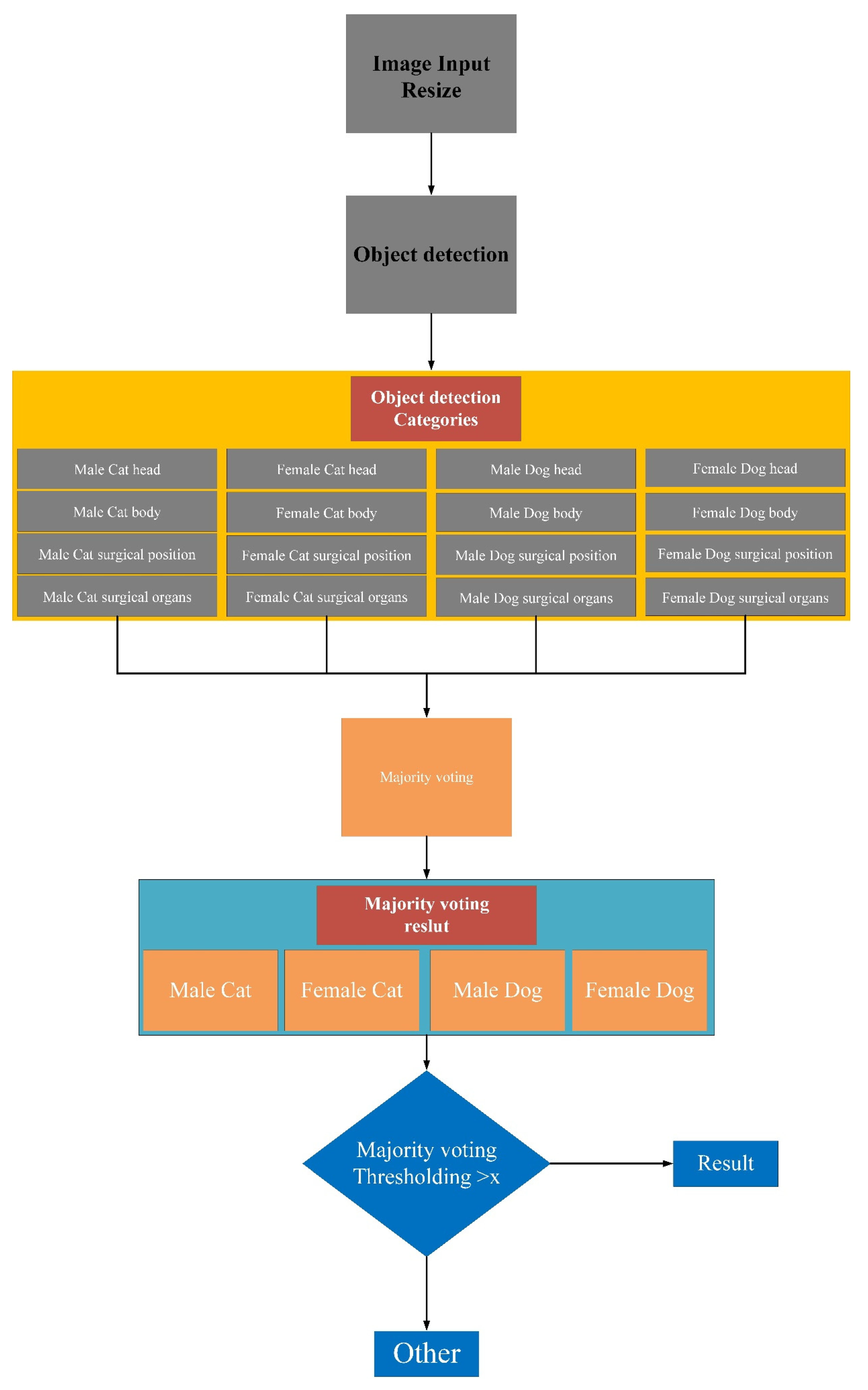
2. Methodology
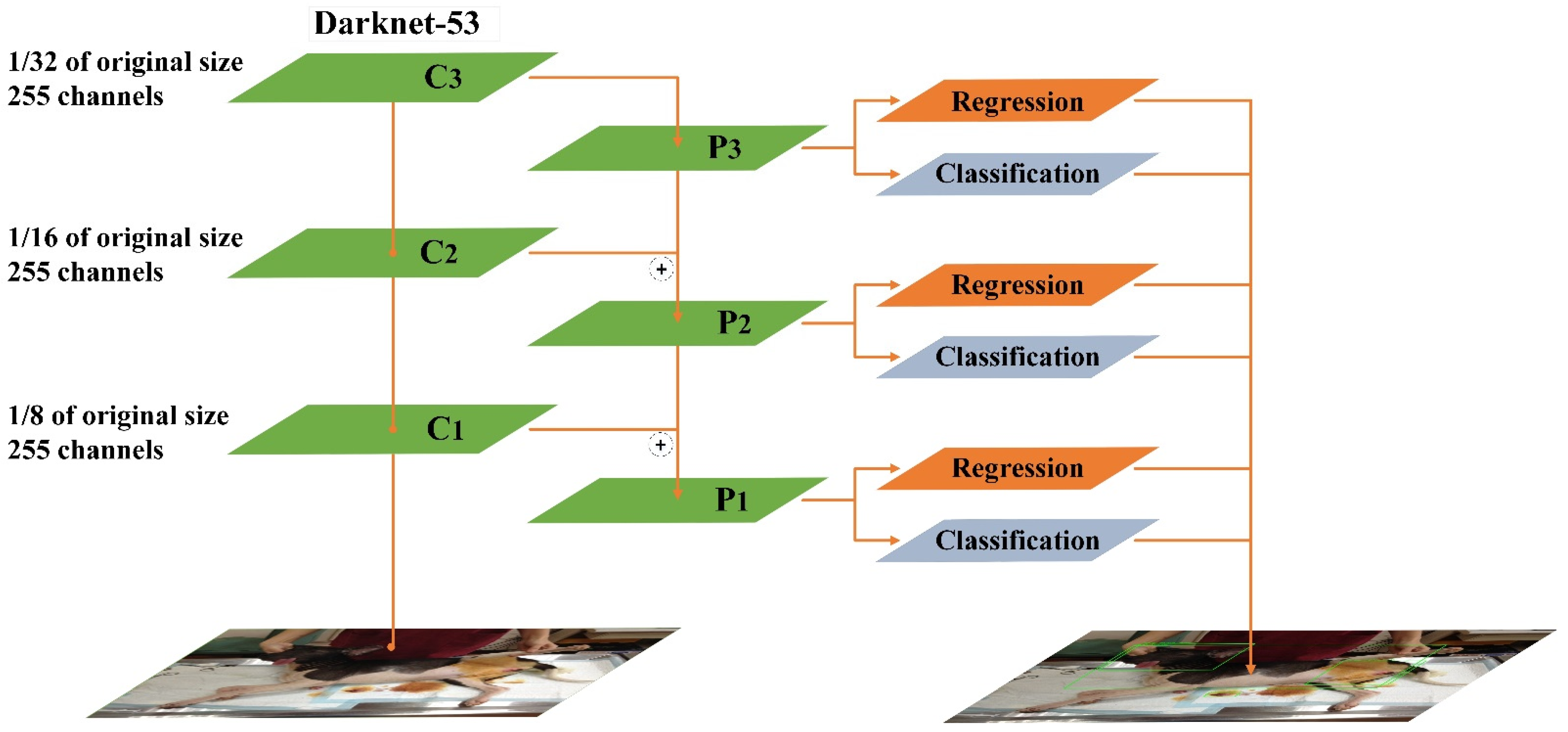
2.1. Yolov3 Deep Learning Network
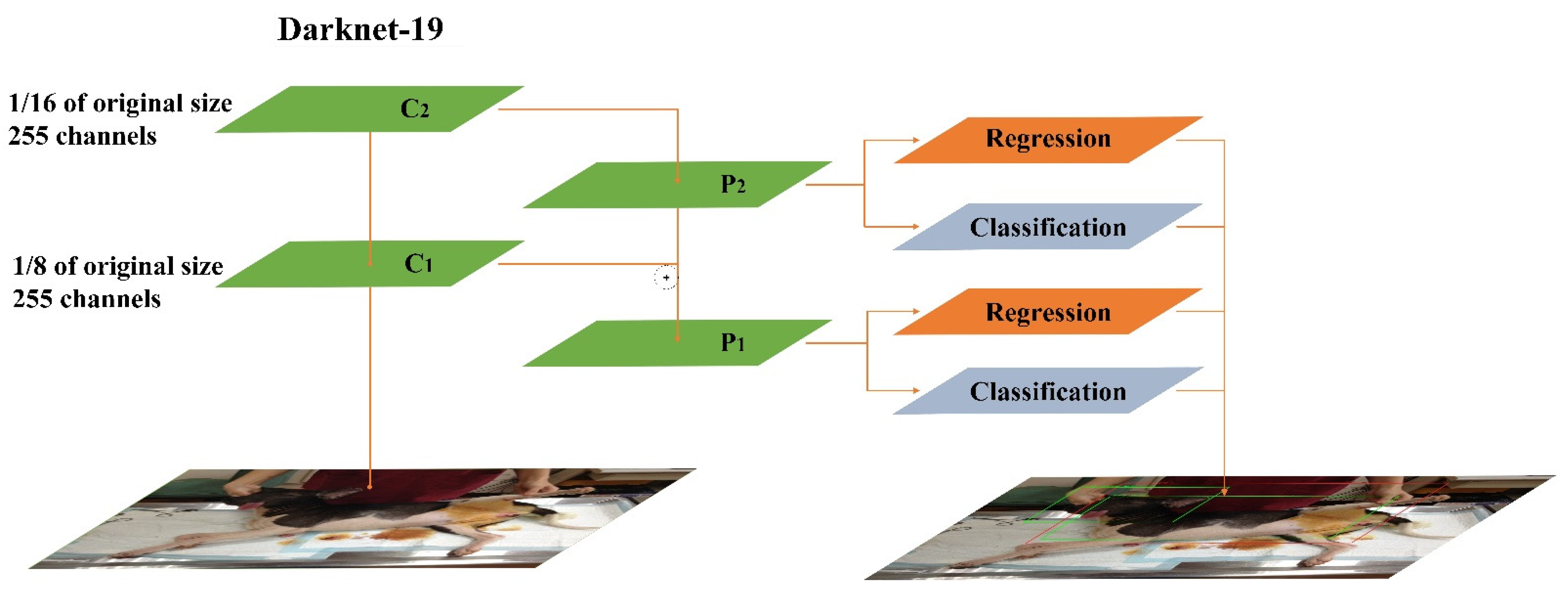
2.2. Yolov3-Tiny Deep Learning Network
2.3. Yolov4 Deep Learning Network
2.4. Basis of Classifier Voting Technique
3. Methods
3.1. Processing
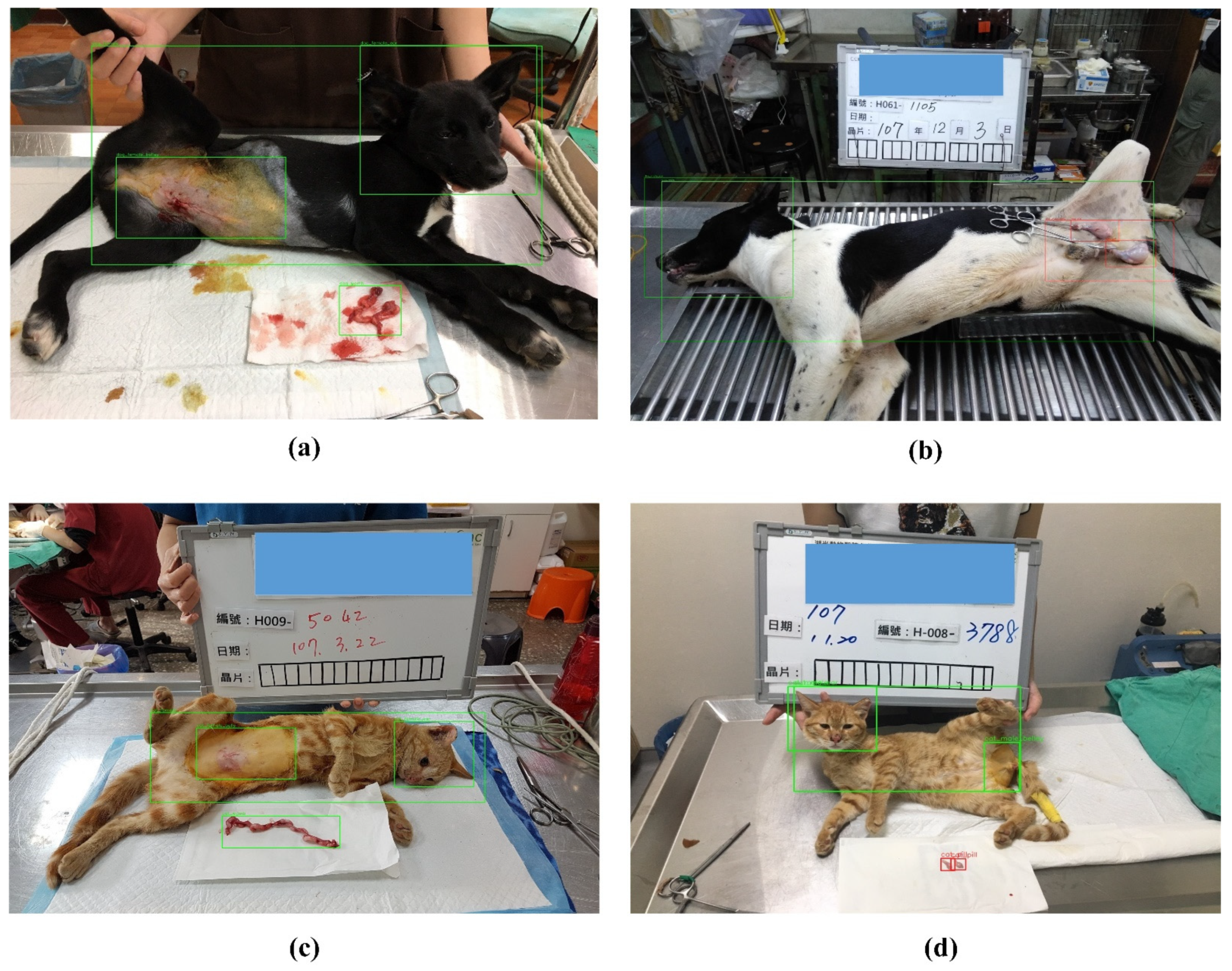
3.2. Dataset Composition and Characteristics
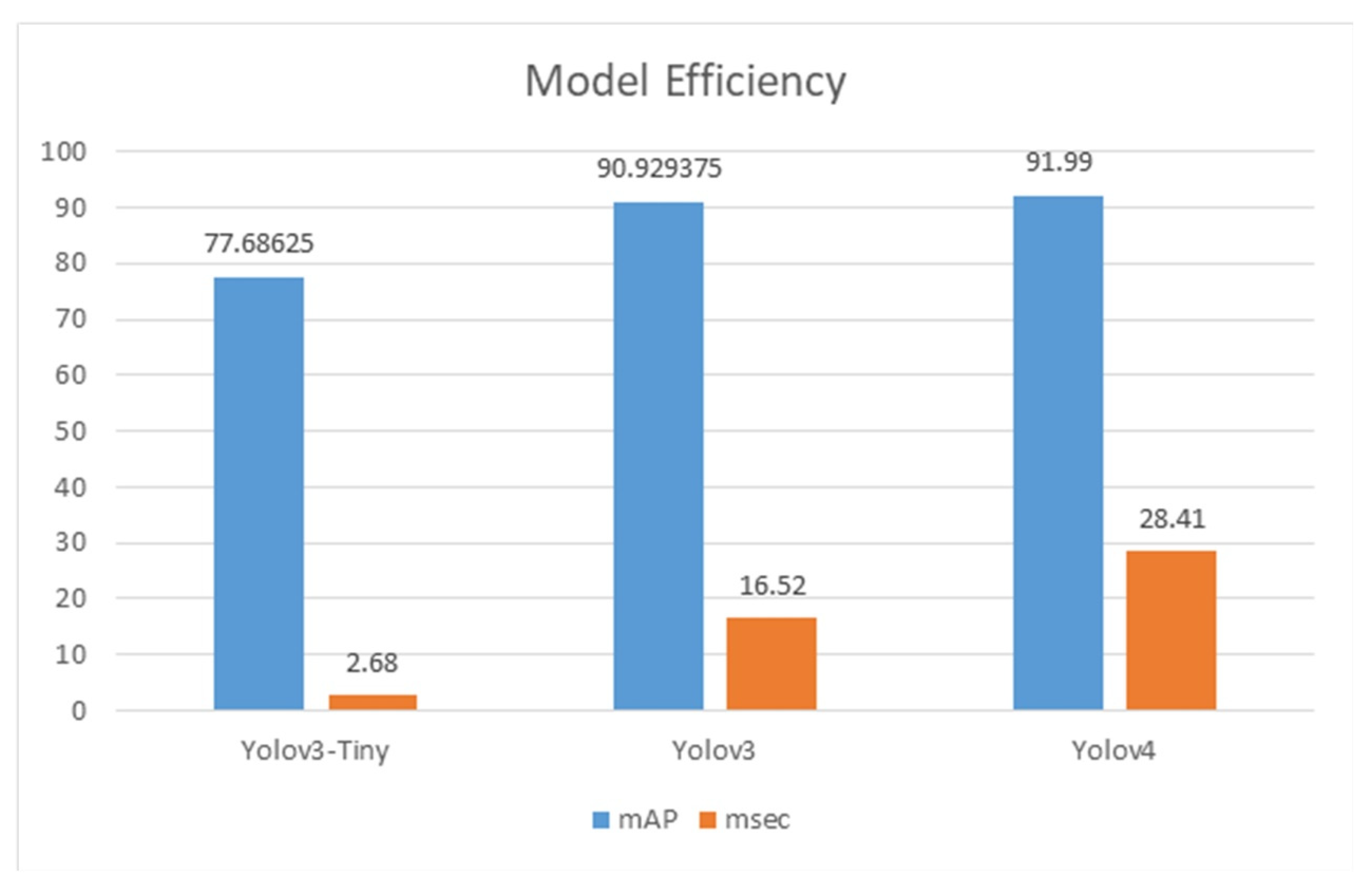
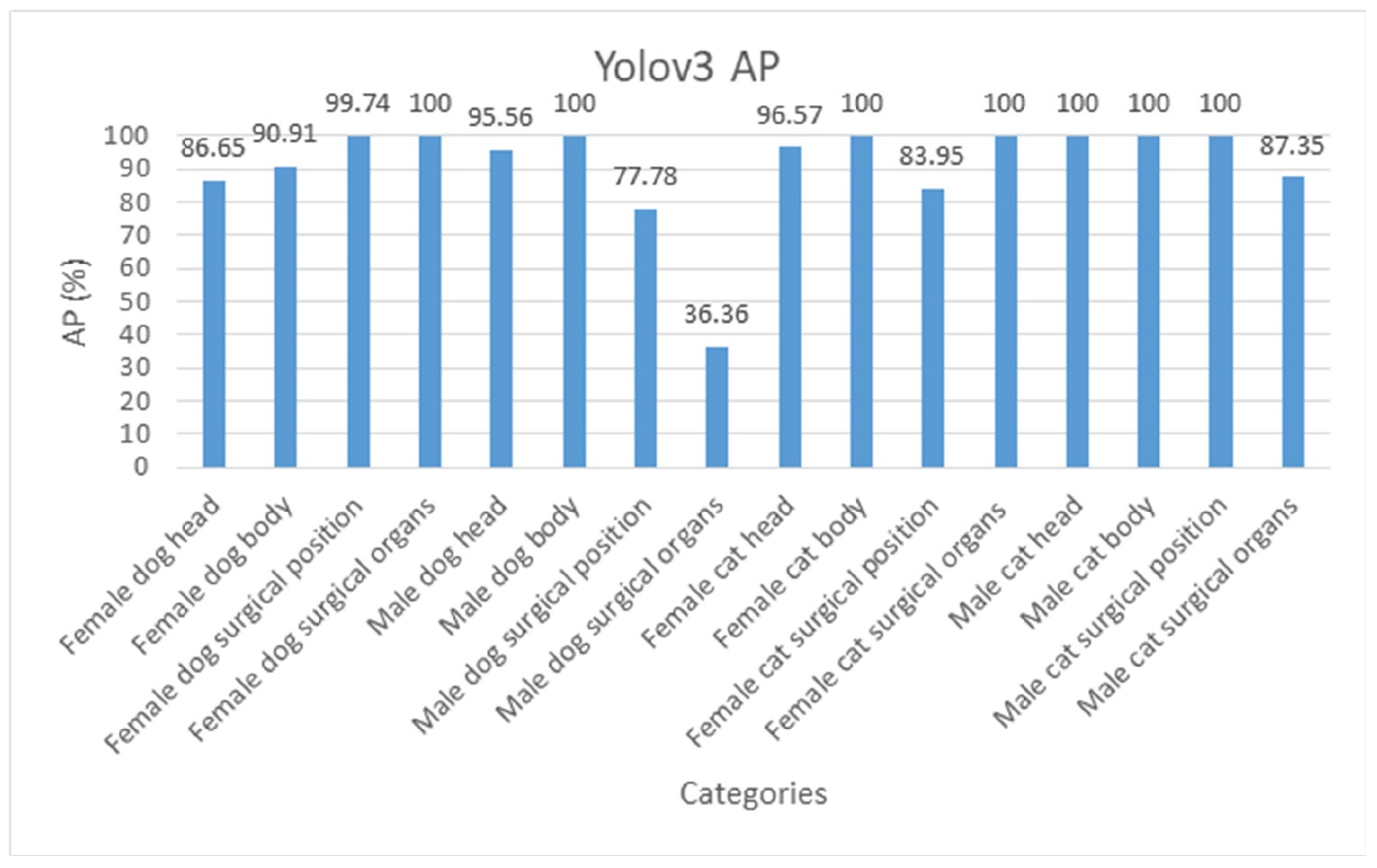
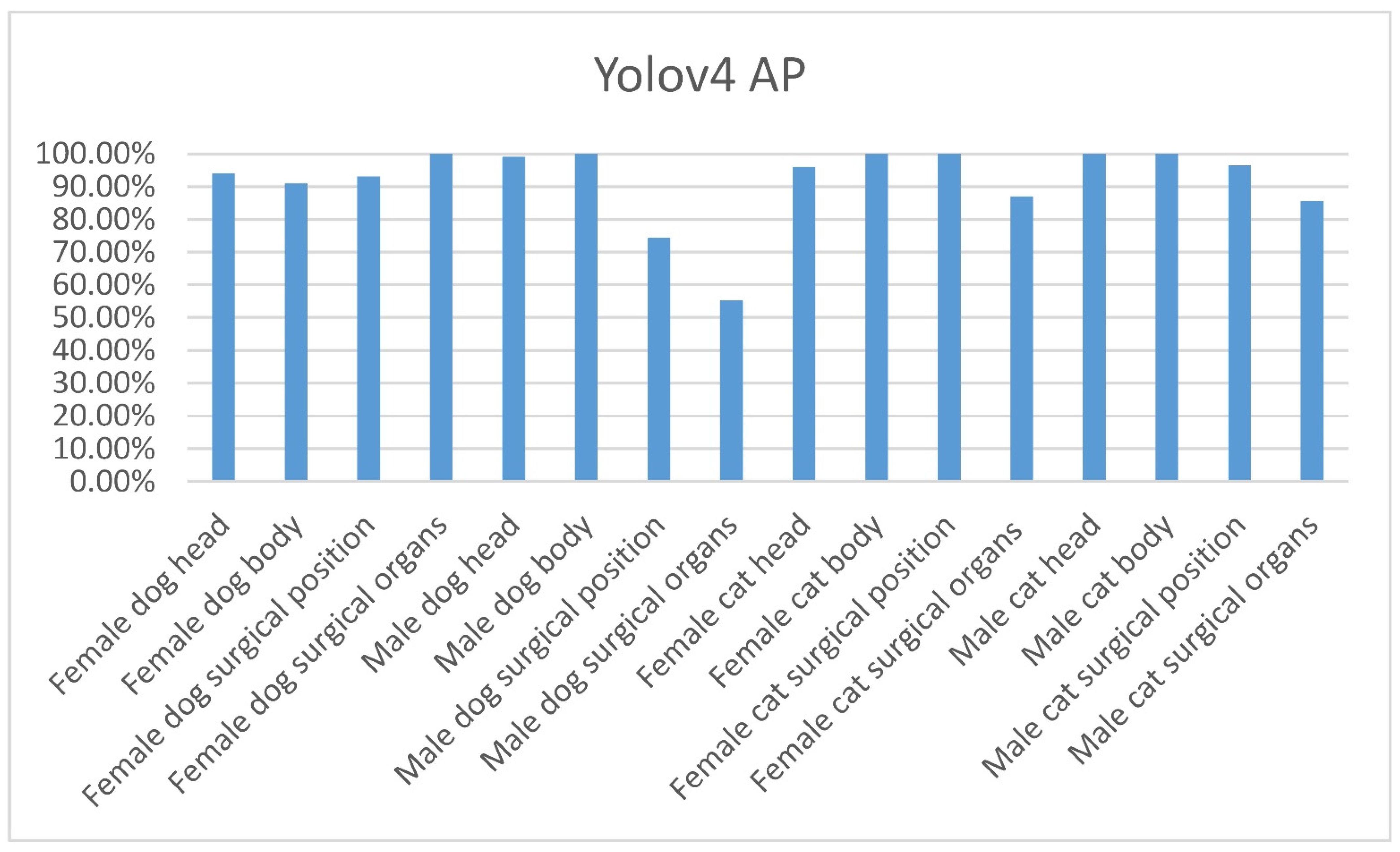
3.3. Detection Performance
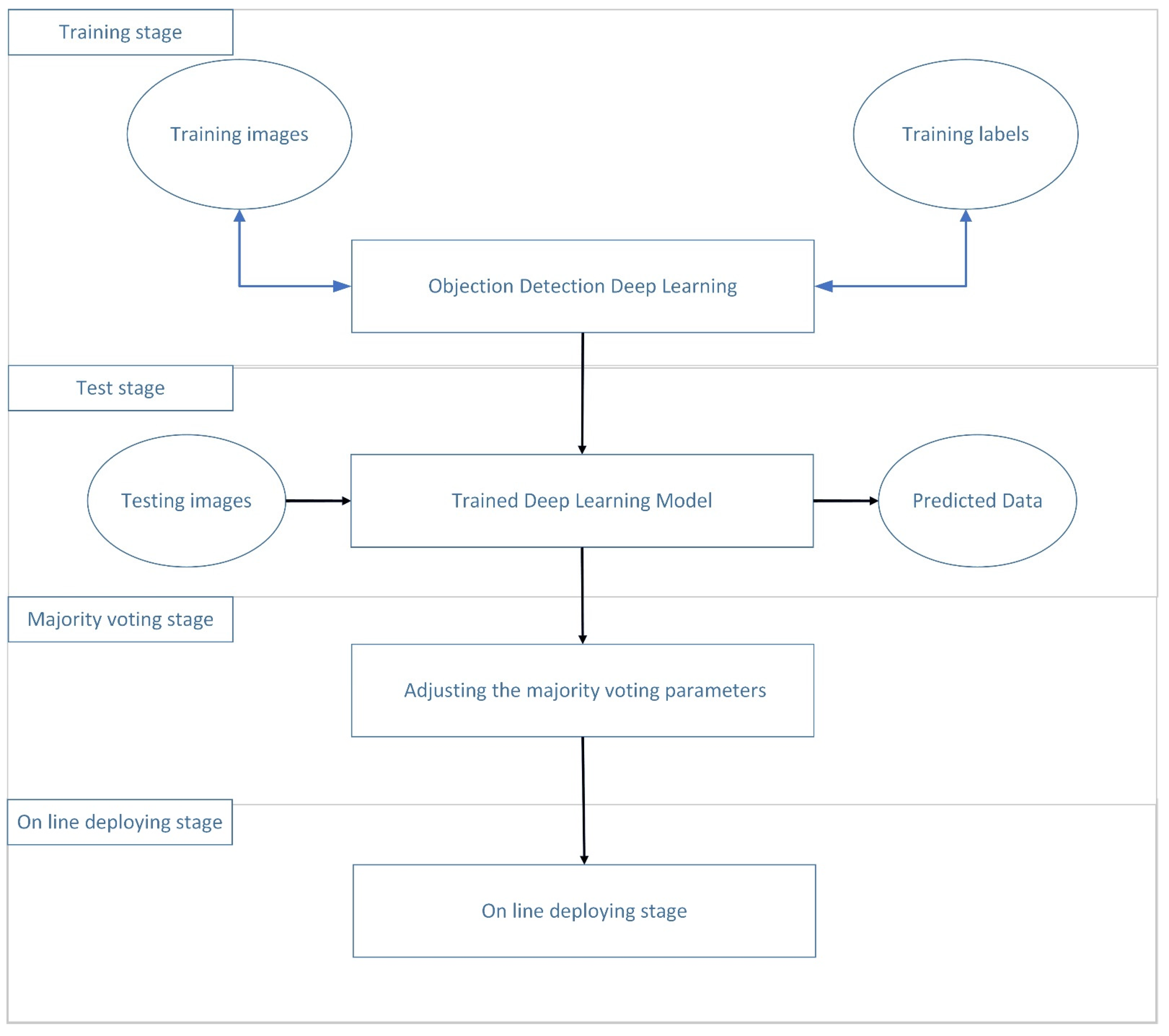
3.4. Majority Voting Algorithm for Classification Results
4. Discussion
4.1. Evaluation Criteria
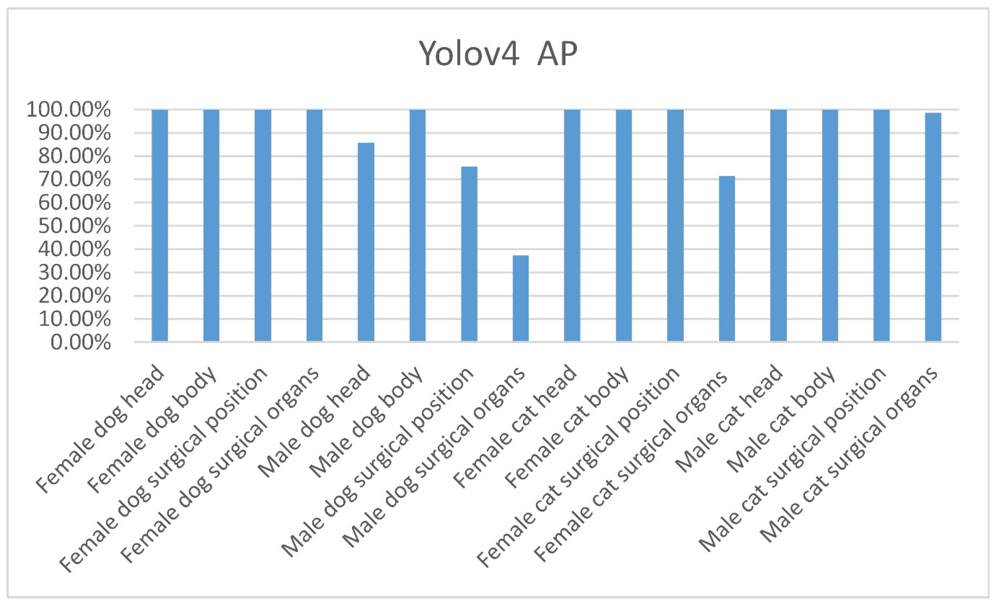
4.2. The Performance of Yolov3-Tiny, Yolov3, and Yolov4
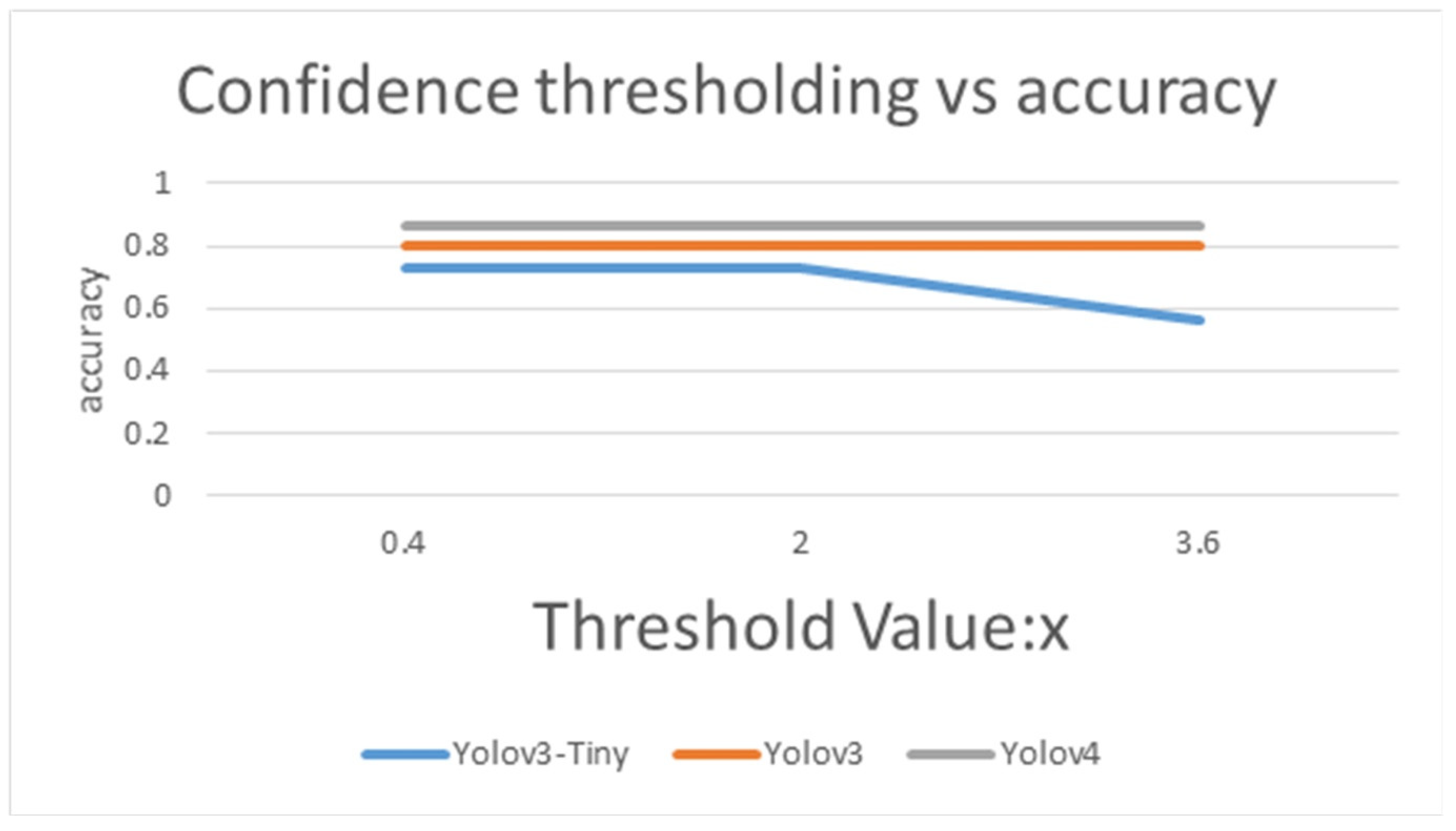
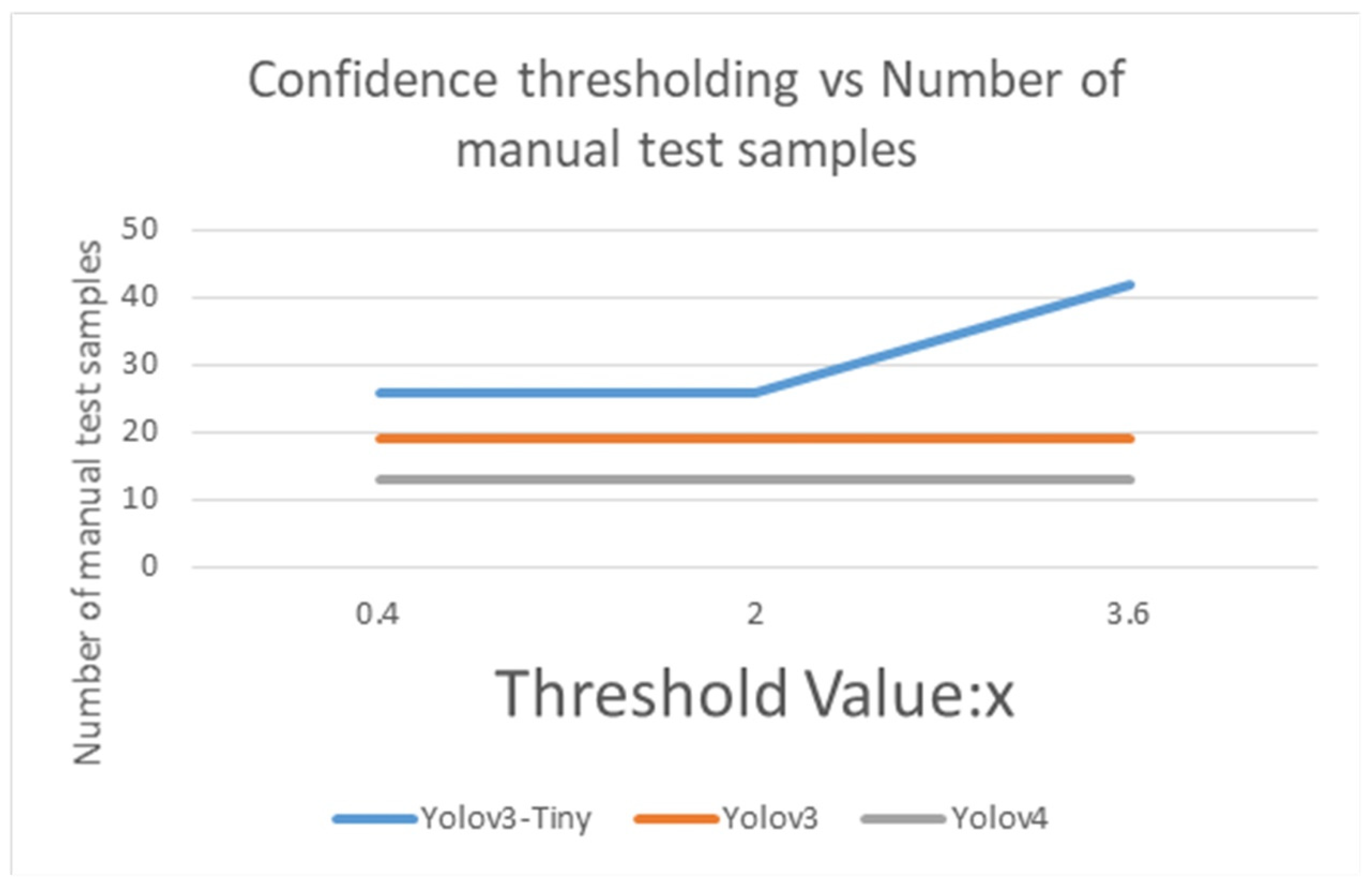
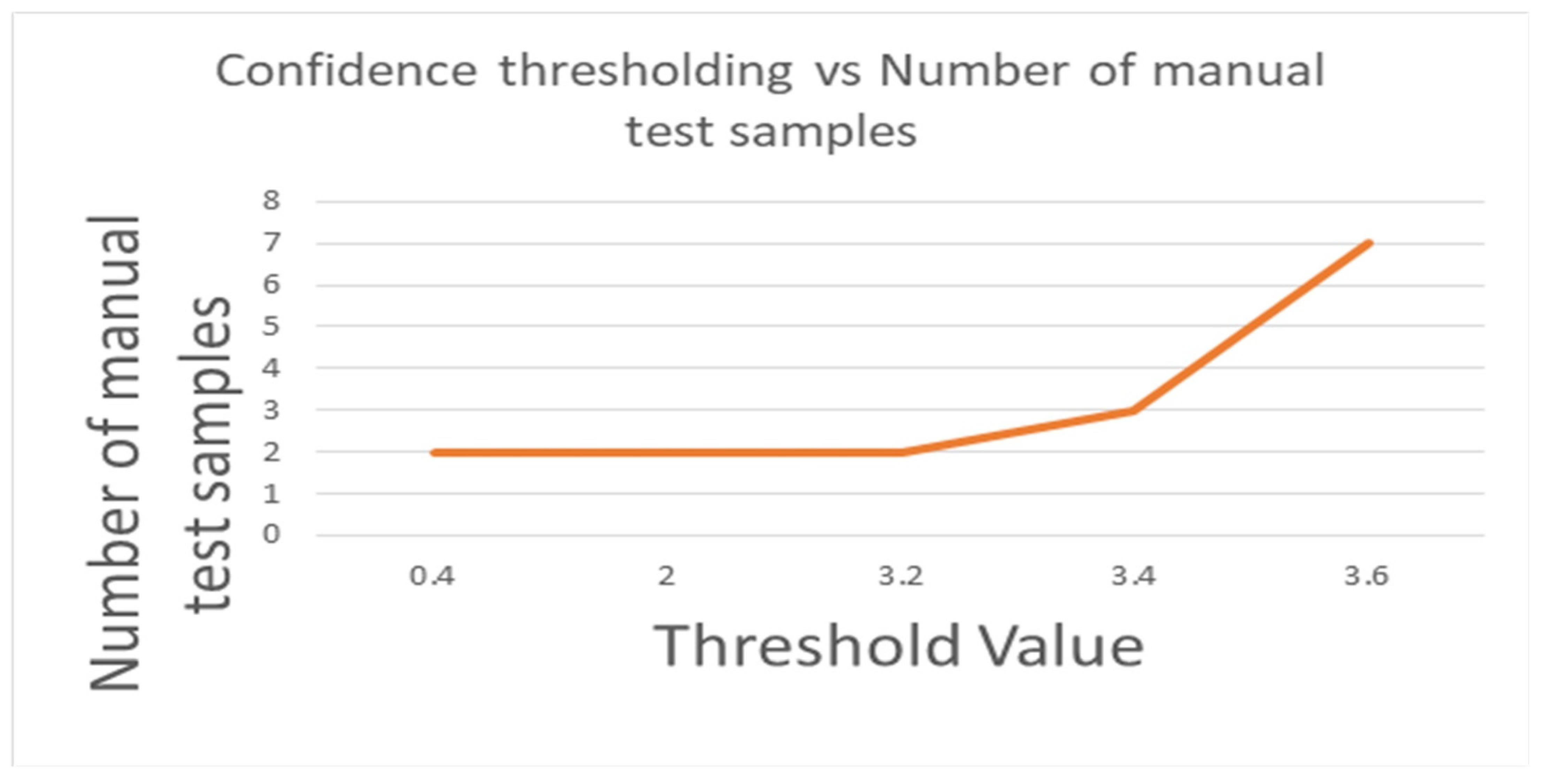
4.3. The Performance and Confidence Thresholding of Majority Voting Multi-Classification by Yolov3-Tiny, Yolov3, and Yolov4
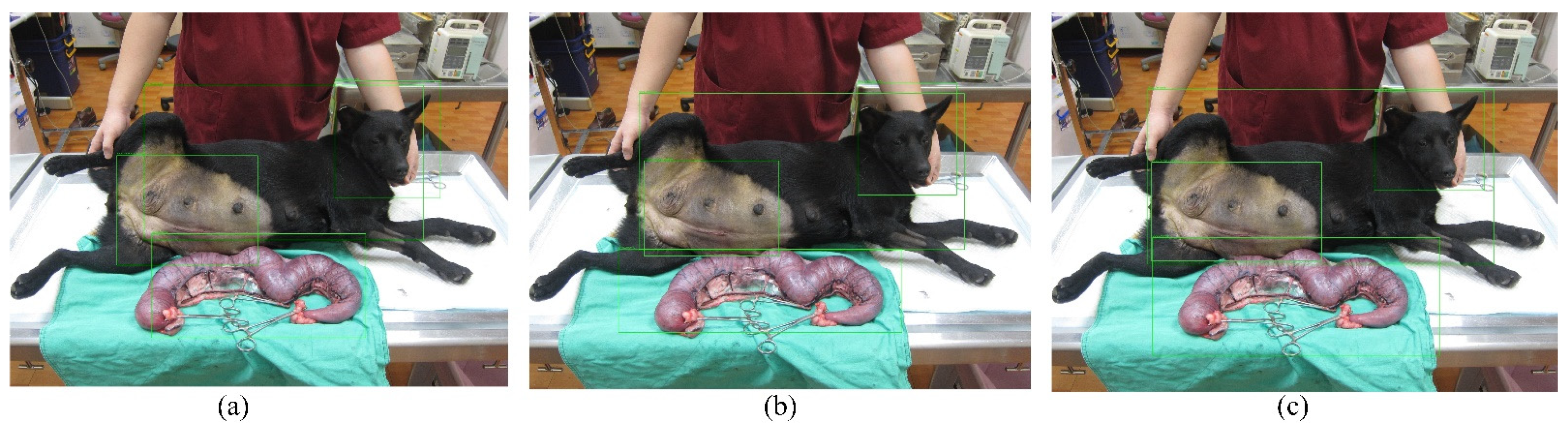
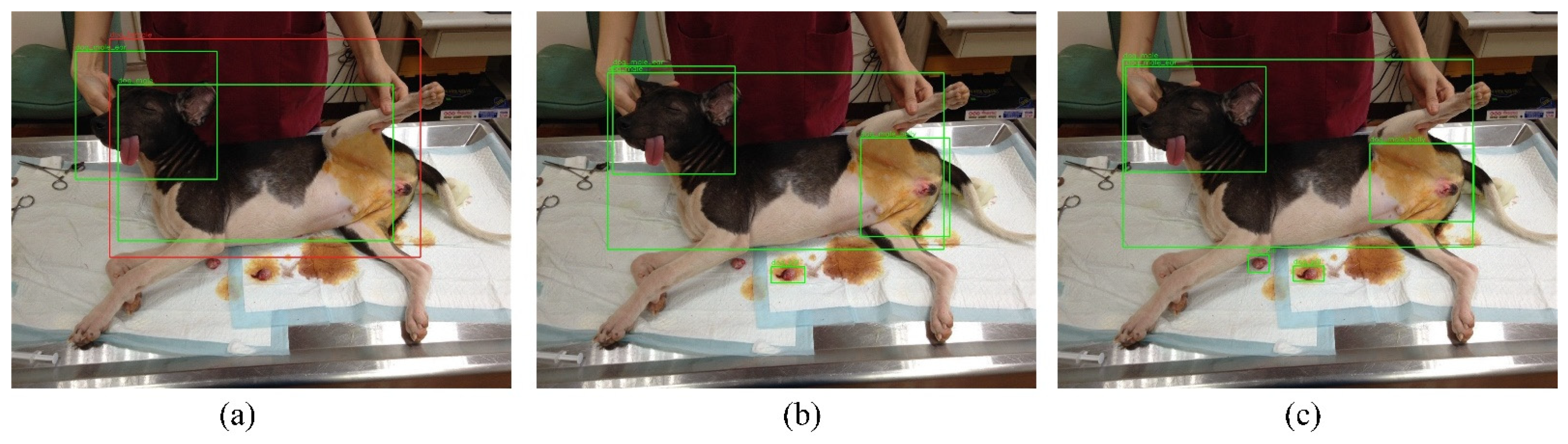
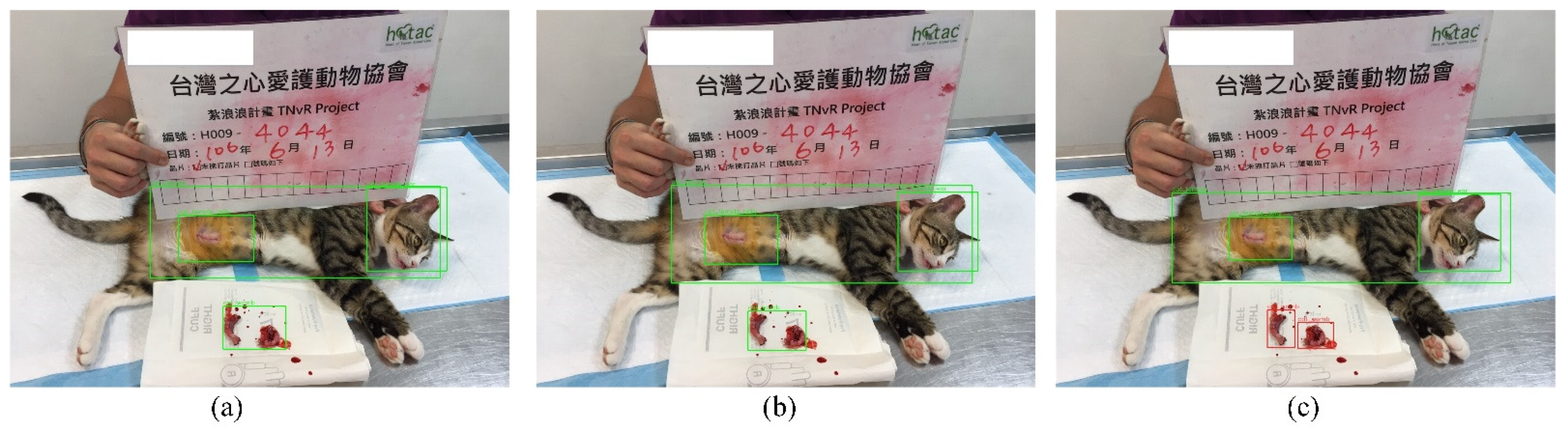
4.4. Special Case Discussion
5. Conclusions
Author Contributions
Funding
Institutional Review Board Statement
Informed Consent Statement
Data Availability Statement
Acknowledgments
Conflicts of Interest
References
- Patronek, G.J. Free-roaming and feral cats—Their impact on wildlife and human beings. J. Am. Vet. Med. Assoc. 1998, 212, 218–226. [Google Scholar] [PubMed]
- Slater, M.R. Community Approaches to Feral Cats; Humane Society Press: Washington, DC, USA, 2002. [Google Scholar]
- Levy, J.; Isaza, N.; Scott, K. Effect of high-impact targeted trap-neuter-return and adoption of community cats on cat intake to a shelter. Vet. J. 2014, 201, 269–274. [Google Scholar] [CrossRef] [PubMed] [Green Version]
- Boone, J.D.; Slater, M.A. A Generalized Population Monitoring Program to Inform the Management of Free-Roaming Cats; Allian Contracept Cats Dogs: Portland, OR, USA, 2014. [Google Scholar]
- Forbush, E.H. The Domestic Cat; Bird Killer, Mouser and Destroyer of Wild Life; Means of Utilizing and Controlling It; Wright & Potter Printing Company: Boston, MA, USA, 1916. [Google Scholar] [CrossRef]
- Grimm, D. Citizen Canine: Our Evolving Relationship with Cats and Dogs; Public Affairs: New York, NY, USA, 2014. [Google Scholar]
- Miller, P.S.; Boone, J.D.; Briggs, J.R.; Lawler, D.F.; Levy, J.K.; Nutter, F.B.; Slater, M.; Zawistowski, S. Simulating free-roaming cat population management options in open demographic environments. PLoS ONE 2014, 9, e113553. [Google Scholar] [CrossRef]
- Bennett, P.; Rohlf, V. Perpetration-induced Traumatic Stress in Persons Who Euthanize Nonhuman Animals in Surgeries, Animal Shelters, and Laboratories. Soc. Anim. 2005, 13, 201–220. [Google Scholar] [CrossRef] [PubMed]
- Reeve, C.L.; Rogelberg, S.G.; Spitzmüller, C.; Digiacomo, N. The Caring-Killing Paradox: Euthanasia-Related Strain Among Animal-Shelter Workers1. J. Appl. Soc. Psychol. 2005, 35, 119–143. [Google Scholar] [CrossRef]
- Frommer, S.S.; Arluke, A. Loving Them to Death: Blame-Displacing Strategies of Animal Shelter Workers and Surrenderers. Soc. Anim. 1999, 7, 1–16. [Google Scholar] [CrossRef]
- Baran, B.E.; Allen, J.A.; Rogelberg, S.G.; Spitzmüller, C.; Digiacomo, N.A.; Webb, J.B.; Carter, N.T.; Clark, O.L.; Teeter, L.A.; Walker, A.G. Euthanasia-related strain and coping strategies in animal shelter employees. J. Am. Vet. Med. Assoc. 2009, 235, 83–88. [Google Scholar] [CrossRef] [Green Version]
- Spehar, D.D.; Wolf, P.J. An Examination of an Iconic Trap-Neuter-Return Program: The Newburyport, Massachusetts Case Study. Animals 2017, 7, 81. [Google Scholar] [CrossRef] [PubMed] [Green Version]
- Spehar, D.D.; Wolf, P.J. A case study in citizen science: The effectiveness of a trap-neuter-return program in a Chicago neigh-borhood. Animals 2018, 8, 14. [Google Scholar] [CrossRef] [PubMed] [Green Version]
- Berkeley, E.P. TNR Past, Present, and Future; Alley Cat Allies: Bethesda, MY, USA, 2004. [Google Scholar]
- Zhao, Z.-Q.; Zheng, P.; Xu, S.-T.; Wu, X. Object Detection With Deep Learning: A Review. IEEE Trans. Neural Netw. Learn. Syst. 2019, 30, 3212–3232. [Google Scholar] [CrossRef] [Green Version]
- Everingham, M.; Van Gool, L.; Williams, C.K.I.; Winn, J.; Zisserman, A. The Pascal Visual Object Classes (VOC) Challenge. Int. J. Comput. Vis. 2009, 88, 303–338. [Google Scholar] [CrossRef] [Green Version]
- Deng, J.; Karpathy, A.; Ma, S.; Russakovsky, O.; Huang, Z.; Bernstein, M.; Krause, J.; Su, H.; Li, F.-F.; Satheesh, S.; et al. ImageNet Large Scale Visual Recognition Challenge. Int. J. Comput. Vis. 2015, 115, 211–252. [Google Scholar] [CrossRef]
- He, K.; Zhang, X.; Ren, S.; Sun, J. Deep residual learning for image recognition. In Proceedings of the IEEE Conference on Computer Vision and Pattern Recognition, Las Vegas, NV, USA, 27–30 June 2016. [Google Scholar]
- Simonyan, K.; Zisserman, A. Very deep convolutional networks for large-scale image recognition. arXiv 2018, arXiv:1409.1556. [Google Scholar]
- Girshick, R.; Donahue, J.; Darrell, T.; Malik, J. Rich feature hierarchies for accurate object detection and semantic segmentation. In Proceedings of the IEEE Conference on Computer Vision and Pattern Recognition, Columbus, OH, USA, 23–28 June 2014. [Google Scholar]
- He, K.; Zhang, X.; Ren, S.; Sun, J. Spatial pyramid pooling in deep convolutional networks for visual recognition. IEEE Trans Pattern Anal. Mach. Intell. 2015, 37, 1904–1916. [Google Scholar] [CrossRef] [PubMed] [Green Version]
- Girshick, R. Fast r-cnn. In Proceedings of the IEEE International Conference on Computer Vision, Las Condes, Chile, 13–16 December 2015. [Google Scholar]
- Ren, S.; He, K.; Girshick, R.; Sun, J. Faster r-cnn: Towards real-time object detection with region proposal networks. Adv. Neural Inform. Process Syst. 2015, 39, 1137–1149. [Google Scholar] [CrossRef] [PubMed] [Green Version]
- Cai, Z.; Vasconcelos, N. Cascade r-cnn: Delving into high quality object detection. In Proceedings of the IEEE Conference on Computer Vision and Pattern Recognition, Salt Lake City, UT, USA, 18–22 June 2018. [Google Scholar]
- Redmon, J.; Divvala, S.; Girshick, R.; Farhadi, A. You only look once: Unified, real-time object detection. In Proceedings of the IEEE Conference on Computer Vision and Pattern Recognition, Las Vegas, NV, USA, 26 June–1 July 2016. [Google Scholar]
- Redmon, J.; Farhadi, A. Yolov3: An incremental improvement. arXiv 2018, arXiv:1804.02767. [Google Scholar]
- Bochkovskiy, A.; Wang, C.Y.; Liao, H.Y.M. YOLOv4: Optimal speed and accuracy of object detection. arXiv 2020, arXiv:2004.10934. [Google Scholar]
- Wang, C.Y.; Liao, H.Y.M.; Wu, Y.H.; Chen, P.Y.; Hsieh, J.W.; Yeh, I.H. CSPNet: A new backbone that can enhance learning capability of CNN. In Proceedings of the IEEE/CVF Conference on Computer Vision and Pattern Recognition Workshops, Seattle, WA, USA, 14–19 June 2020. [Google Scholar]
- Lin, T.Y.; Dollár, P.; Girshick, R.; He, K.; Hariharan, B.; Belongie, S. Feature pyramid networks for object detection. In Proceedings of the IEEE Conference on Computer Vision and Pattern Recognition, Honolulu, HI, USA, 21–26 July 2017. [Google Scholar]
- Liu, W.; Anguelov, D.; Erhan, D.; Szegedy, C.; Reed, S.; Fu, C.Y.; Berg, A.C. SSD: Single Shot Multibox Detector. In European Conference on Computer Vision; Springer: Cham, Switzerland, 2016. [Google Scholar]
- Lin, T.Y.; Goyal, P.; Girshick, R.; He, K.; Dollár, P. Focal loss for dense object detection. In Proceedings of the IEEE International Conference on Computer Vision, Venice, Italy, 22–29 October 2017. [Google Scholar]
- He, K.; Gkioxari, G.; Dollár, P.; Girshick, R. Mask r-cnn. In Proceedings of the IEEE International Conference on Computer Vision, Venice, Italy, 22–29 October 2017. [Google Scholar]
- Nguyen, H.; Maclagan, S.J.; Nguyen, T.D.; Nguyen, T.; Flemons, P.; Andrews, K.; Ritchie, E.G.; Phung, D. Animal Recognition and Identification with Deep Convolutional Neural Networks for Automated Wildlife Monitoring. In Proceedings of the 2017 IEEE International Conference on Data Science and Advanced Analytics, Tokyo, Japan, 19–21 October 2017; pp. 40–49. [Google Scholar] [CrossRef]
- Villa, A.G.; Salazar, A.; Vargas, F. Towards automatic wild animal monitoring: Identification of animal species in camera-trap images using very deep convolutional neural networks. Ecol. Inform. 2017, 41, 24–32. [Google Scholar] [CrossRef] [Green Version]
- Zeppelzauer, M. Automated detection of elephants in wildlife video. EURASIP J. Image Video Process. 2013, 2013, 46. [Google Scholar] [CrossRef] [Green Version]
- Hsing, P.; Bradley, S.; Kent, V.T.; Hill, R.; Smith, G.; Whittingham, M.J.; Cokill, J.; Crawley, D.; Stephens, P.; MammalWeb Volunteers. Economical crowdsourcing for camera trap image classification. Remote Sens. Ecol. Conserv. 2018, 4, 361–374. [Google Scholar] [CrossRef]
- Delahay, R.J.; Cox, R. Wildlife surveillance using deep learning methods. Ecol. Evol. 2019, 9, 9453–9466. [Google Scholar]
- Spampinato, C.; Farinella, G.M.; Boom, B.; Mezaris, V.; Betke, M.; Fisher, R. Special issue on animal and insect behaviour under-standing in image sequences. EURASIP J. Image Video Process. 2015, 1–4. [Google Scholar] [CrossRef] [Green Version]
- Dalal, N.; Triggs, B. Histograms of oriented gradients for human detection. In Proceedings of the 2005 IEEE Computer Society Conference on Computer Vision and Pattern Recognition (CVPR’05), San Diego, CA, USA, 20–25 June 2005; Volume 1. [Google Scholar]
- Zhu, H.; Yuen, K.-V.; Mihaylova, L.; Leung, H. Overview of Environment Perception for Intelligent Vehicles. IEEE Trans. Intell. Transp. Syst. 2017, 18, 2584–2601. [Google Scholar] [CrossRef] [Green Version]
- Islam, S.S.; Dey, E.K.; Tawhid, M.N.A.; Hossain, B.M. A CNN Based Approach for Garments Texture Design Classification. Adv. Technol. Innov. 2017, 2, 119. [Google Scholar]
- Ho, C.-C.; Su, E.; Li, P.-C.; Bolger, M.J.; Pan, H.-N. Machine Vision and Deep Learning Based Rubber Gasket Defect Detection. Adv. Technol. Innov. 2020, 5, 76–83. [Google Scholar] [CrossRef]
- Krizhevsky, A.; Sutskever, I.; Hinton, G.E. ImageNet classification with deep convolutional neural networks. Commun. ACM 2017, 60, 84–90. [Google Scholar] [CrossRef]
- Willi, M.; Pitman, R.T.; Cardoso, A.W.; Locke, C.; Swanson, A.; Boyer, A.; Veldthuis, M.; Fortson, L. Identifying animal species in camera trap images using deep learning and citizen science. Methods Ecol. Evol. 2018, 10, 80–91. [Google Scholar] [CrossRef] [Green Version]
- Norouzzadeh, M.S.; Nguyen, A.; Kosmala, M.; Swanson, A.; Palmer, M.S.; Packer, C.; Clune, J. Automatically identifying, counting, and describing wild animals in camera-trap images with deep learning. Proc. Natl. Acad. Sci. USA 2018, 115, E5716–E5725. [Google Scholar] [CrossRef] [Green Version]
- Zhou, Z.H. Ensemble Methods: Foundations and Algorithms; CRC Press: Boca Raton, FL, USA, 2012. [Google Scholar]
- Kuncheva, L.I. Combining Pattern Classifiers: Methods and Algorithms; John Wiley & Sons: Hoboken, NJ, USA, 2014. [Google Scholar]
- Freung, Y.; Shapire, R. A decision-theoretic generalization of on-line learning and an application to boosting. J. Comput. Syst. Sci. 1997, 55, 119–139. [Google Scholar] [CrossRef] [Green Version]
 refers to the aggregation operation.
refers to the aggregation operation.
refers to the aggregation operation.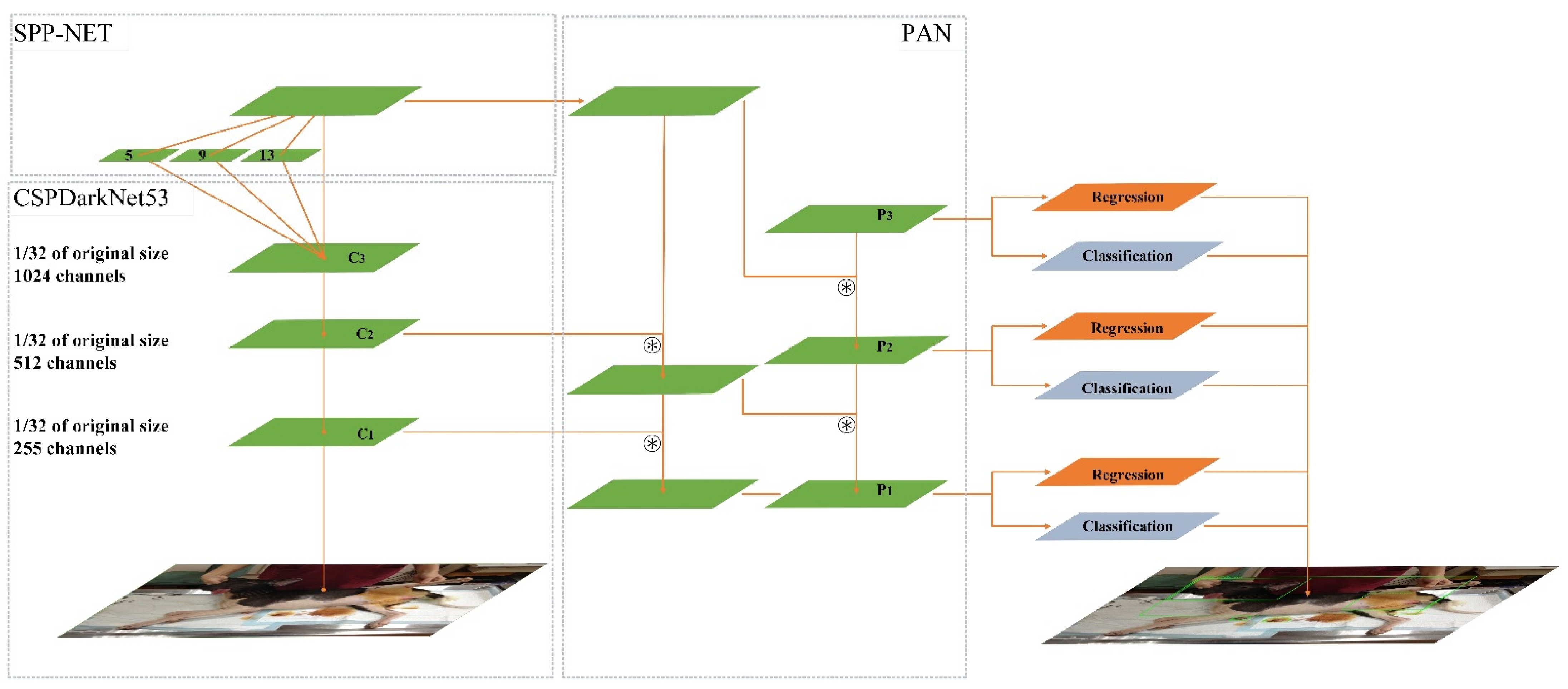


| Classification Neural Network | Object Detection Network | Semantic Recognition Neural Network | |
|---|---|---|---|
| Can it locate the object area? | No | Yes | Yes |
| Image label time | Short | within 1 min | 3 to 5 min |
| Class | Train | Test |
|---|---|---|
| Dog male | 73 | 11 |
| Dog female | 101 | 19 |
| Cat male | 266 | 29 |
| Cat female | 373 | 37 |
| Total | 813 | 96 |
| Yolov3-Tiny | Yolov3 | Yolov4 | |
|---|---|---|---|
| Head of female dog | 0.9994 | 0.9999 | 0.9997 |
| Body of female dog | 0.9858 | 1.0000 | 0.9986 |
| Surgical position of female dog | 0.9941 | 1.0000 | 0.9926 |
| Surgical organs of female dog | 0.9869 | 0.9959 | 0.9774 |
| Yolov3-Tiny | Yolov3 | Yolov4 | |
|---|---|---|---|
| Head of male dog | 0.8001 | 0.9948 | 0.9996 |
| Body of male dog | 0.4046 | 0.9993 | 0.9979 |
| Surgical position of male dog | Null | 0.9995 | 0.9974 |
| Surgical organs of male dog | Null | 0.9835 | 0.8059/0.9804 |
| Body of female dog | 0.3417 |
| Yolov3-Tiny | Yolov3 | Yolov4 | |
|---|---|---|---|
| Head of female cat | 0.9996 | 1.0000 | 0.9991 |
| Body of female cat | 0.9997 | 0.9997 | 0.9998 |
| Surgical position of female cat | 0.9914 | 0.9998 | 0.9988 |
| Surgical organs of female cat | 0.8308 | 0.9961 | 0.8912/0.5778 |
| Yolov3-Tiny | Yolov3 | Yolov4 | |
|---|---|---|---|
| Head of male cat | 0.9998 | 1.0000 | 0.9963 |
| Body of male cat | 0.9993 | 0.9995 | 0.9999 |
| Surgical position of male cat | 0.9539 | 1.0000 | 0.9961 |
| Surgical organs of male cat | 0.9487/0.9135 | 1.0000/0.9999 | 0.9964/0.9966 |
| Yolov3-Tiny | Yolov3 | Yolov4 | |
|---|---|---|---|
| Male dog | 1.2047 | 3.9711 | 4.96 |
| Female dog | 0.3417 | ||
| Categories result | “Other” | Male dog | Male dog |
| Yolov3-Tiny | Yolov3 | Yolov4 | |
|---|---|---|---|
| Female dog | 3.9662 | 3.9958 | 3.9683 |
| Classification result | Female Dog | Female Dog | Female Dog |
| Yolov3-Tiny | Yolov3 | Yolov4 | |
|---|---|---|---|
| Female cat | 3.8215 | 3.9956 | 4.4667 |
| Classification result | Female cat | Female cat | Female cat |
| Yolov3-Tiny | Yolov3 | Yolov4 | |
|---|---|---|---|
| Male cat | 4.8152 | 4.9994 | 4.9853 |
| Classification result | Male cat | Male cat | Male cat |
| mAP(%) | Detection Time (msec) | |
|---|---|---|
| Yolov3-Tiny | 54.19 | 2.68 |
| Yolov3 | 93.99 | 16.52 |
| Yolov4 | 62.8 | 28.41 |
| Categories | AP(%) |
|---|---|
| Head of female dogs | 54.19 |
| Body of female dogs | 88.43 |
| Surgical position of female dogs | 76.92 |
| Surgical organs of female dogs | 77.28 |
| Head of male dogs | 60 |
| Body of male dogs | 63.75 |
| Surgical position of male dogs | 60 |
| Surgical organs male dogs | 31.82 |
| Head of female cats | 93.99 |
| Body of female cats | 100 |
| Surgical position of female cats | 100 |
| Surgical organs of female cats | 78.72 |
| Head of male cats | 95.08 |
| Body of male cats | 100 |
| Surgical position of male cats | 100 |
| Surgical organs male cats | 62.8 |
| mAP (%) | 77.68 |
| Male Dog | Female Dog | Male Cat | Female Cat | Accuracy | Mean Accuracy | |
|---|---|---|---|---|---|---|
| Male dog | 2 | 0.73 | 0.6 | |||
| Female dog | 7 | |||||
| Male cat | 27 | |||||
| Female cat | 34 | |||||
| “Other” | 9 | 12 | 2 | 3 | ||
| Individual accuracy | 0.18 | 0.37 | 0.93 | 0.92 |
| Male Dog | Female Dog | Male Cat | Female Cat | Accuracy | Mean Accuracy | |
|---|---|---|---|---|---|---|
| Male dog | 4 | 0.802 | 0.6875 | |||
| Female dog | 8 | |||||
| Male cat | 28 | |||||
| Female cat | 37 | |||||
| “Other” | 7 | 11 | 1 | |||
| Individual accuracy | 0.36 | 0.42 | 0.97 | 1 |
| Male Dog | Female Dog | Male Cat | Female Cat | Accuracy | Mean Accuracy | |
|---|---|---|---|---|---|---|
| Male dog | 9 | 0.85 | 0.795 | |||
| Female dog | 1 | 7 | ||||
| Male cat | 29 | |||||
| Female cat | 37 | |||||
| “Other” | 1 | 12 | ||||
| Individual accuracy | 0.81 | 0.37 | 1 | 1 |
| Class | Train | Test |
|---|---|---|
| Dog male | 64 | 7 |
| Dog female | 64 | 7 |
| Cat male | 64 | 7 |
| Cat female | 64 | 7 |
| Total | 256 | 28 |
| Male Dog | Female Dog | Male Cat | Female Cat | Accuracy | Mean Accuracy | |
|---|---|---|---|---|---|---|
| Male dog | 5 | 0.92 | 0.92 | |||
| Female dog | 7 | |||||
| Male cat | 7 | |||||
| Female cat | 7 | |||||
| “Other” | 2 | |||||
| Individual accuracy | 0.71 | 1 | 1 | 1 |
Publisher’s Note: MDPI stays neutral with regard to jurisdictional claims in published maps and institutional affiliations. |
© 2021 by the authors. Licensee MDPI, Basel, Switzerland. This article is an open access article distributed under the terms and conditions of the Creative Commons Attribution (CC BY) license (https://creativecommons.org/licenses/by/4.0/).
Share and Cite
Huang, Y.-C.; Chuang, T.-H.; Lai, Y.-L. Classification of the Trap-Neuter-Return Surgery Images of Stray Animals Using Yolo-Based Deep Learning Integrated with a Majority Voting System. Appl. Sci. 2021, 11, 8578. https://doi.org/10.3390/app11188578
Huang Y-C, Chuang T-H, Lai Y-L. Classification of the Trap-Neuter-Return Surgery Images of Stray Animals Using Yolo-Based Deep Learning Integrated with a Majority Voting System. Applied Sciences. 2021; 11(18):8578. https://doi.org/10.3390/app11188578
Chicago/Turabian StyleHuang, Yi-Cheng, Ting-Hsueh Chuang, and Yeong-Lin Lai. 2021. "Classification of the Trap-Neuter-Return Surgery Images of Stray Animals Using Yolo-Based Deep Learning Integrated with a Majority Voting System" Applied Sciences 11, no. 18: 8578. https://doi.org/10.3390/app11188578
APA StyleHuang, Y.-C., Chuang, T.-H., & Lai, Y.-L. (2021). Classification of the Trap-Neuter-Return Surgery Images of Stray Animals Using Yolo-Based Deep Learning Integrated with a Majority Voting System. Applied Sciences, 11(18), 8578. https://doi.org/10.3390/app11188578