Article

A Waste Classification Method Based on a Multilayer Hybrid Convolution Neural Network

1
College of Communication and Electronic Engineering, Qiqihar University, Qiqihar 161000, China
2
College of Information and Communication Engineering, Dalian Nationalities University, Dalian 116000, China
*
Author to whom correspondence should be addressed.
Appl. Sci. 2021, 11(18), 8572; https://doi.org/10.3390/app11188572
Submission received: 22 August 2021 / Revised: 4 September 2021 / Accepted: 8 September 2021 / Published: 15 September 2021
(This article belongs to the Special Issue Advances in Waste Treatment and Material Recycling)

Abstract

:
With the rapid development of deep learning technology, a variety of network models for classification have been proposed, which is beneficial to the realization of intelligent waste classification. However, there are still some problems with the existing models in waste classification such as low classification accuracy or long running time. Aimed at solving these problems, in this paper, a waste classification method based on a multilayer hybrid convolution neural network (MLH-CNN) is proposed. The network structure of this method is similar to VggNet but simpler, with fewer parameters and a higher classification accuracy. By changing the number of network modules and channels, the performance of the proposed model is improved. Finally, this paper finds the appropriate parameters for waste image classification and chooses the optimal model as the final model. The experimental results show that, compared with some recent works, the proposed method has a simpler network structure and higher waste classification accuracy. A large number of experiments in a TrashNet dataset show that the proposed method achieves a classification accuracy of up to 92.6%, which is 4.18% and 4.6% higher than that of some state-of-the-art methods, and proves the effectiveness of the proposed method.

1. Introduction

Waste classification and recycling plays a very important role in daily life. With the improvement of people’s living standards, an increasing amount of daily waste is produced. Facing the situation of increasing waste discharge and environmental degradation, how to classify waste accurately, maximize the utilization of waste resources, and improve the quality of the living environment are urgent issues of common concern in the world. Waste classification technology is used to classify and control waste at the source, turning it into resources again through later classification and recycling. In the past, waste classification required a lot of manpower and material resources. With the development of artificial intelligence, deep learning and intelligent technologies have been widely used. Intelligent waste classification has become an important technology in waste management. Intelligent waste classification can be applied to mobile devices, intelligent recyclable trash cans, etc. It is beneficial to the environment and improves the recycling of waste resources. How to improve its classification performance on a dataset with few samples and a large similarity between classes still requires the further exploration. For the TrashNet dataset, which has a small amount of data, a waste classification method based on a multilayer hybrid convolution neural network (MLH-CNN) is proposed. By way of mixing modules, this paper finds the appropriate classification parameters on the TrashNet dataset and chooses the optimal model as the final model. Moreover, the influence of optimizers on waste image classification is analyzed and the best possible optimizer is selected. Compared with some state-of-the-art methods, the proposed MLH-CNN network has a simper structure and fewer parameters, and can provide better classification performance for waste images.

2. Related Work

In the previous research, waste classification methods can be divided into two categories: traditional methods and neural network methods.

2.1. Based on Traditional Methods

In 1999, Lulea University of Technology launched a project to develop a system for recycling metal waste using mechanical shape identifiers [1]. In a Bayesian computing framework, sift and contour features were used, and the system was based on the Flickr material database [2]. Jinqiang Bai et al. designed a new waste collection robot. The robot could use deep neural networks to detect waste autonomously [3]. Artzai Picon et al. proposed a fuzzy spectrum and spatial classifier algorithm that combined spectral and spatial features, reducing the dimension of hyperspectral data by constructing spectral fuzzy sets of organisms. The experimental results showed that the classification rate was greatly improved when spectral spatial features were used for nonferrous metal waste [4]. Reference [5] showed that there were different ways to solve the class imbalance problem, and that there was a trend towards the usage of patterns and fuzzy approaches due to the favorable results. Reference [6] also introduced the role of fuzzy logic in artificial neural network (ANN). At the same time, this paper describes the application of neural network in a chemical technology system. S. Shylo et al. utilized millimeter wave imaging technology with multiple sensors to provide complementary data, thus improving its classification performance for waste paper and cards [7]. Rutqvist D et al. exploited an automatic machine learning method to solve the container-emptying problem of intelligent waste management systems.
Using an existing artificial engineering model and an improved traditional machine learning algorithm, a random forest classifier was used to achieve the best effect and improve the prediction quality of the emptying time of the recycling container [8]. Zheng, J.J. et al. proposed to use a mathematical statistics method to express individual bounded rationality and to use the specific graph structure of a scale-free network to represent the group structure. This paper has certain theoretical value for the representation of individual bounded rationality; at the same time, it has a promotion effect on waste classification [9]. Chu Y et al. proposed a multilayer hybrid deep learning system, which could automatically classify waste disposed by individuals in urban public areas. The multilayer perceptual machine (MLP) method was used to integrate image features and other feature information, and good classification performance was obtained [10].

2.2. Based on Neural Network Methods

In 2016, a system that automatically identified compost waste was proposed by TensorFlow of Google. The disadvantage of this system is that it can only distinguish compost materials [11,12]. In 2012, Alex Krizhevsky et al. proposed AlexNet, which achieved good results in the image classification task. Since then, good convolutional neural networks have been proposed, which can be used for target detection and classification [13]. Noushin Karimian et al. proposed a new classification method that used magnetic induction spectroscopy to classify three metals and could construct an effective classifier [14]. Zhao Dong-e et al. used a hyperspectral imaging system to collect waste samples, and preprocessed the samples for denoising and correction, which could obtain more accurate classification results [15]. Yusoff. S. H et al. designed a system that could automatically separate recyclable metal household waste [16]. Zeng et al. proposed a method to detect large-area waste distribution by hyperspectral data. A new hyperspectral image classification network was designed, which performed well in large-area waste detection [17]. SeokBeom Roh et al. used hybrid technology to construct a radial basis function neural network classifier, which could effectively recycle waste [18].
Kennedy et al. exploited the Visual Geometry Group 19(VGG-19)VGG-19 [19] as the basic model of transfer learning; the classification accuracy of waste images was 88.42%, making good use of the ability of VGG-19 to extract features [20]. Adeeji et al. used the convolution neural network model constructed by the 50-layer residual network preprocessing (ResNet-50 [21]) as the extractor, and utilized the support vector machine (SVM [22]) to classify, achieving an accuracy of 87% on the waste image dataset [23]. Chen Zhihong et al. proposed a grab system for waste using an automatic sorting robot based on computer vision. In order to achieve an accurate grab of target objects, the Region Proposal Network (RPN) [24] and VGG-16 [19] models were used for object recognition and attitude estimation [25]. Stephen L. and others used MobileNet [26] to generate the model, which also exploited transferred learning for the Imagenet large-scale visual recognition challenge, and obtained an 87.2% accuracy. After optimization and quantification at a later stage, the accuracy rate reached 89.34%, and it was successfully applied to mobile devices [27]. The residual network [28], which was first proposed by Dr. He Kaiming, showed excellent results on Imagenet in 2015. However, with the deepening of the model, the learning ability will also appear with a “degradation”; that is, when the model level is deepened, the error rate will increase. Therefore, the network is not suitable for waste classification with few datasets. Ruiz V. and others exploited the advantages of the classical deep learning models and compared different deep learning systems in the automatic classification of waste types. The optimal combination of the ResNet [29] model concept achieved 88.60% accuracy on waste images [30]. Costa et al. studied different types of neural networks and divided the waste images into four categories; among the different neural networks, the accuracies of the K Nearest Neighbors (KNN) [31], SVM, and RandomF (RF) pretraining model methods were 88.0%, 80.0%, and 85.0%, respectively [32].
Traditional machine learning technologies require the calibration of a large number of training data, which will consume a lot of manpower and material resources. Traditional machine learning algorithms such as MLP, KNN, and RF perform a large amount of calculation and cannot fit the data and balance the samples well. Therefore, the traditional machine learning algorithm is not suitable for waste classification. Among the neural network waste classification methods, most use the classic convolution neural networks for fine-tuning or pre-training on large datasets. However, the method of pre-training and fine-tuning contains a large number of parameters, and fine-tuning on small datasets may lead to overestimation or underestimation. The literature [33] shows that the application of the pre-training model and fine-tuning on small datasets may not be the best way to fit the data. Moreover, the waste classification performance of the above literature is not adequate. To solve these problems, a convolutional neural network with a simple structure and a few parameters is proposed in this paper. For the TrashNet dataset with few samples, a network with a complex structure or a large network is not suitable. The network structure proposed in this paper is similar to that of Visual Geometry Group Network (VggNet) but simpler, with fewer parameters and higher classification accuracy. By changing the number of network modules and channels, the performance of the model is improved. Finally, this paper finds the appropriate parameters for waste image classification and chooses the optimal model as the final model.
The main contributions of this paper are as follows:
(1)
We analyze the characteristics of the TrashNet dataset and give the reason why the classical convolution neural network based on fine-tuning is not suitable for waste image classification;
(2)
We proposed a multilayer hybrid convolutional neural network method (MLH-CNN), which can provide the best classification performance by changing the number of network modules and channels. Meanwhile, the influence of optimizers on waste image classification is also analyzed and the best possible optimizer is selected;
(3)
Compared with some state-of-the-art methods, the proposed MLH-CNN network has a simper structure and fewer parameters, and can provide better classification performance for waste images.
The rest of this paper is organized as follows. Section 3 explains the methodology, and Section 4 presents the experiments and the analysis. Finally, the conclusions are provided in Section 5.

3. Methodology

The overall structure of the proposed method for waste image classification is shown in Figure 1. First, the waste images are preprocessed. Secondly, some image features are extracted by the designed network model. Then, the extracted image features are normalized. Finally, the Softmax classifier is used to classify the waste images. In this section, the designed network model and its improvement process are described in detail.

3.1. The Initial Network Modules

In this paper, the convolution layer and the batch normalization (BN) layer are mainly used to extract image features. The BN [34] layer is used to improve the generalization ability of the network, disturb the training data, and accelerate the convergence speed of the model. During the process of training, BN is calculated based on each small batch. The mean and variance corresponding to each batch of data during training are recorded and used to calculate the mean and variance of the entire training set, which is performed as follows:
μ β = 1 m i = 0 m x i , δ 2 = 1 m x i μ β 2
E x E β μ β , V a r x m m 1 E β δ β 2
where m refers to small batch size, β is a dataset with batch size m , and x is the input of one layer. Batch standardization is carried out for each feature map, i.e., the same operation is taken for batch standardization in different positions of each feature map. Supposing the size of the feature map is p × q , BN for this feature map will be equivalent to normalizing the feature batch with size m = β = m · p q . BN is selected to effectively avoid gradient disappearance and explosion, which has little to do with the initial values of the parameters and has a regularization effect.
In VGGNet, it was pointed out that two 3 × 3 convolution kernels have the same perceptual field of view as one 5 × 5 convolution kernel. Therefore, using a 3 × 3 convolution kernel does not only ensure the perceptual field of view, but also reduces the parameters of the convolution layer. Thus, the 3 × 3 convolution kernels are used in the network structure of this paper.
The structure of the proposed module is shown in Figure 2. Using such modules for mixing, the number of channels per module is 32, 64, 128, 256, etc. Supposing the input layer of the module is the l 1 layer, its input feature map is X l 1 , the corresponding feature convolution kernel is K l , the output of the convolution layer is Z l , and the bias unit of the output layer is b l ; then, the output of the convolution layer will be as follows:
Z u , v l = i = j = X i + u , j + v l 1 · K l · χ ( i , j ) + b l
χ ( i , j ) = 1 , 0 i , j n 0 , o t h e r s
The output feature of the convolution layer passes through the BN layer, and then through the maximum pooling layer for down-sampling. Now, the weight of each unit of convolution kernel is β l + 1 , and a bias unit b l + 1 is added to the output. The output of the sampling layer is as follows:
Z i , j l + 1 = β l + 1 · u = i r ( i + 1 ) r 1 v = j r ( j + 1 ) r 1 a u , v l + b l + 1
a u , v l = f Z u , v l
a i , j l + 1 = f Z i , j l + 1
The sampling layer is followed by the convolution layer; now, the output is the following:
Z u , v l + 2 = i = j = a i + u , j + v l + 1 · K i , j l + 2 · χ ( i , j ) + b l + 2
where X is a matrix of order m × m , K is a matrix of order n × n , a u , v l is a function of Z u , v l , and a i , j l + 1 is a function of Z i , j l + 1 . The range of ( u , v ) is 0 u , v n .
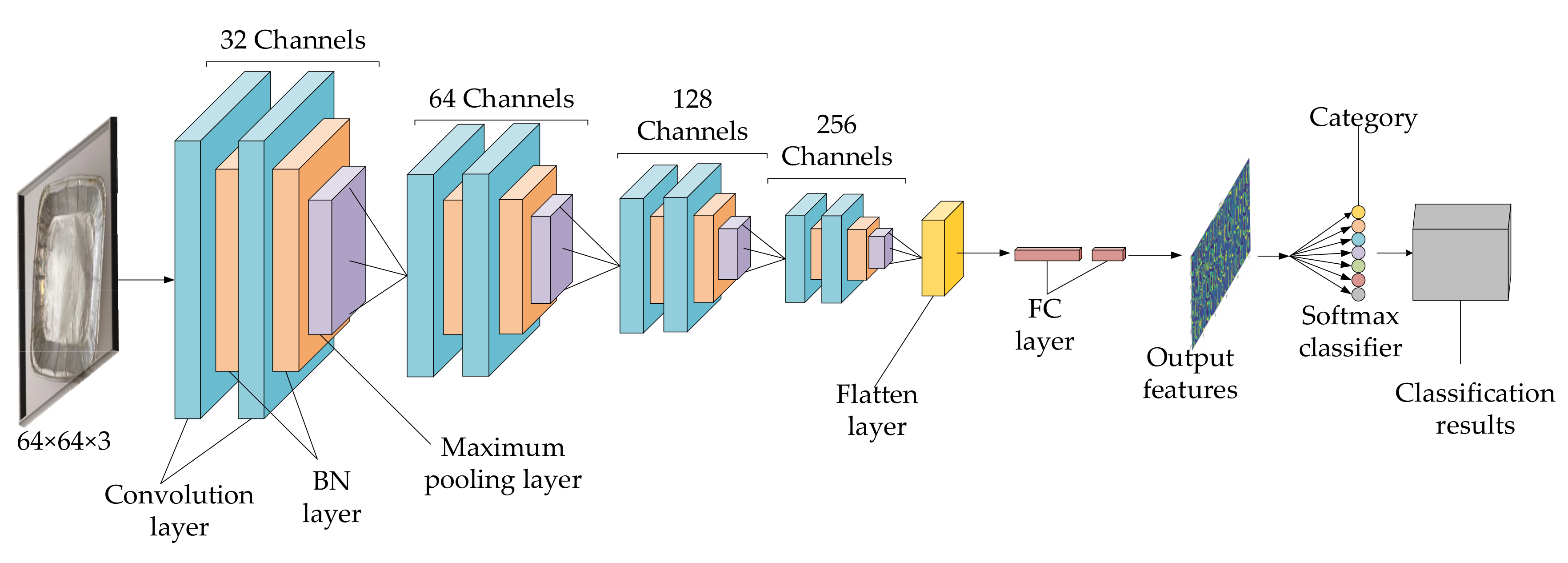
After the modules are mixed, a flattening layer is used, which is used for the transition between the convolution layer and the full connection layer, to “flatten” the data input into the full connection layer. Next, two full connection layers are used, and the number of channels in each full connection layer is 128 and 64. Compared with the large number of channels, the parameters and calculation amount are reduced. Finally, the Softmax classifier is used for classification.
Most of the recent research methods adopt fine-tuning classical convolutional neural networks to classify waste images. However, fine-tuning convolutional neural networks have some shortcomings, such as high complexity and a large number of parameters, which lead to the low accuracy of waste classification. For the TrashNet dataset, convolutional neural networks with high complexity and a large number of parameters are not very suitable. This paper starts with a convolutional neural network with low complexity, few parameters, and a simple structure, and uses a 3 × 3 small convolution kernel to enhance the receptive field of view and reduce the network parameters. As shown in Figure 2, a maximum pool layer is added after every two basic modules, which is used to compress data and reduce the amount of parameters. This can also retain the main features, reduce the amount of computation, and improve the generalization ability of the model. Based on the characteristics of the TrashNet dataset a simple module is designed in this study to improve the performance of waste classification.

3.2. Methods and Improvements

The structures of the initial network model and some of its improved versions are listed in Table 1. The activation function adopted is Relu. The training accuracy and average iteration time of each model are shown in Table 1. The improved process contributes to analyzing and adjusting the depth of the network, finding the appropriate classification network, and obtaining the best classification accuracy.
Based on the above comparison and analysis, the final network structure adopted in this paper is shown in Figure 3. This network structure is composed of four modules. Each convolution layer adopts a small 3 × 3 convolution kernel with a stride of 1. In order to solve the problem of pixels at the corners of the image being omitted during each convolution operation, which leads to the loss of feature information of the image edge, 0 padding is utilized for each convolution layer. The maximum pool layer adopts 2 × 2 filters and 2 × 2 steps. Finally, the total number of parameters of the output network is 17,099.26, which is very small compared with the deep convolution neural network.

3.3. Selection of Optimizer

The optimizer plays an extremely important role in the training of the network model, which is related to whether the training can converge quickly and achieve higher accuracy and recall rate. Common optimizers include Adam, Gradientdescent, and Momentum. In this paper, Adam [35], the stochastic gradient descent method (SGD) [36], and stochastic gradient descent with momentum (SGDM) + Nesterov are mainly studied and compared based on the proposed model.
Under the same conditions, results of the comparison of Adam, SGD, and SGDM + Nesterov with the proposed model are shown in Figure 4. As shown in Figure 4, the effect of SGD in the early stage is the best; Adam and SGD tend to be gradually more stable with the increase in training times, and SGDM + Nesterov has the best effect in the late stage of training. On the whole, SGDM + Nesterov shows good performance in classification accuracy.
The accuracy and the average iteration time of the three optimizers are listed in Table 2. It is obvious that the accuracy and the average iteration time of the SGDM + Nesterov optimizer are the best. Thus, SGDM + Nesterov is adopted as the optimizer and is used to classify features obtained by the proposed model.
In this paper, an image size of 64 × 64 × 3 is used as the model input so as to further reduce the amount of parameters and shorten the training time greatly. The SGDM is chosen as the optimizer, in which the momentum parameter is set to 0.9, the learning rate is set to 0.1, and the Nesterov momentum is adopted. In addition, an early stop mechanism and a learning rate reduction mechanism are added. In this paper, the patience value is set to 30 times. When the loss function value corresponding to the current learning rate is not less than the loss function value corresponding to the previous learning rate, the training is stopped after 30 times under the current learning rate. Under the current learning rate, if the loss function value of the last training is not lower than that of the previous training, the learning rate decreases by 0.1. The batch size is set to 32. The proposed model is developed based on Keras, and the training is completed on GeForce 940MX NVIDIA. Table 3 lists the hyper-parameters of this network.

4. Experiments and Results Analysis

In this part, the TrashNet dataset [37] is first preprocessed. Secondly, the designed model is evaluated on the TrashNet dataset with some evaluation indexes. Finally, the classification performance of the proposed model is compared with that of other methods under the same conditions.

4.1. Dataset Processing

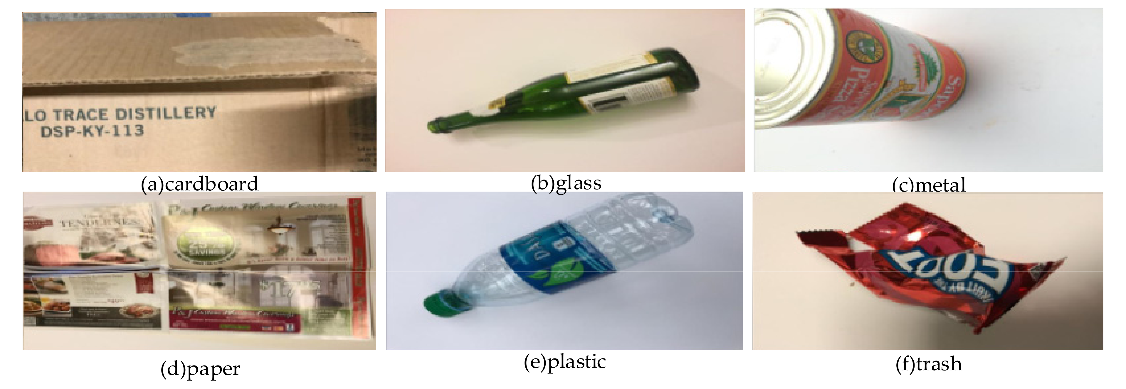
The waste image dataset used in this paper is the TrashNet dataset. The dataset was created by Mindy Yang and Gary Thung of Stanford University, which contains six types of waste images, with a total of 2527 images, including 403 images of cardboard, 501 of glass, 410 of metal, 594 of paper, 482 of plastic, 137 of trash; they are 513 × 384 image pixels. The visualization of the TrashNet dataset is shown in Figure 5. The dataset has a small number of samples for each category; in this paper, under-sampling is used to eliminate the data imbalance to some extent; the waste images are entered into the network with a size of 64 × 64. Additionally, in this study, the number of images in the TrashNet dataset is first determined, and the dataset is subsequently divided into a training set and a test set. The number of categories per dataset is listed in Table 4, and the balance of data is further enhanced by a reasonable number of categories.

4.2. Training Curve Analysis

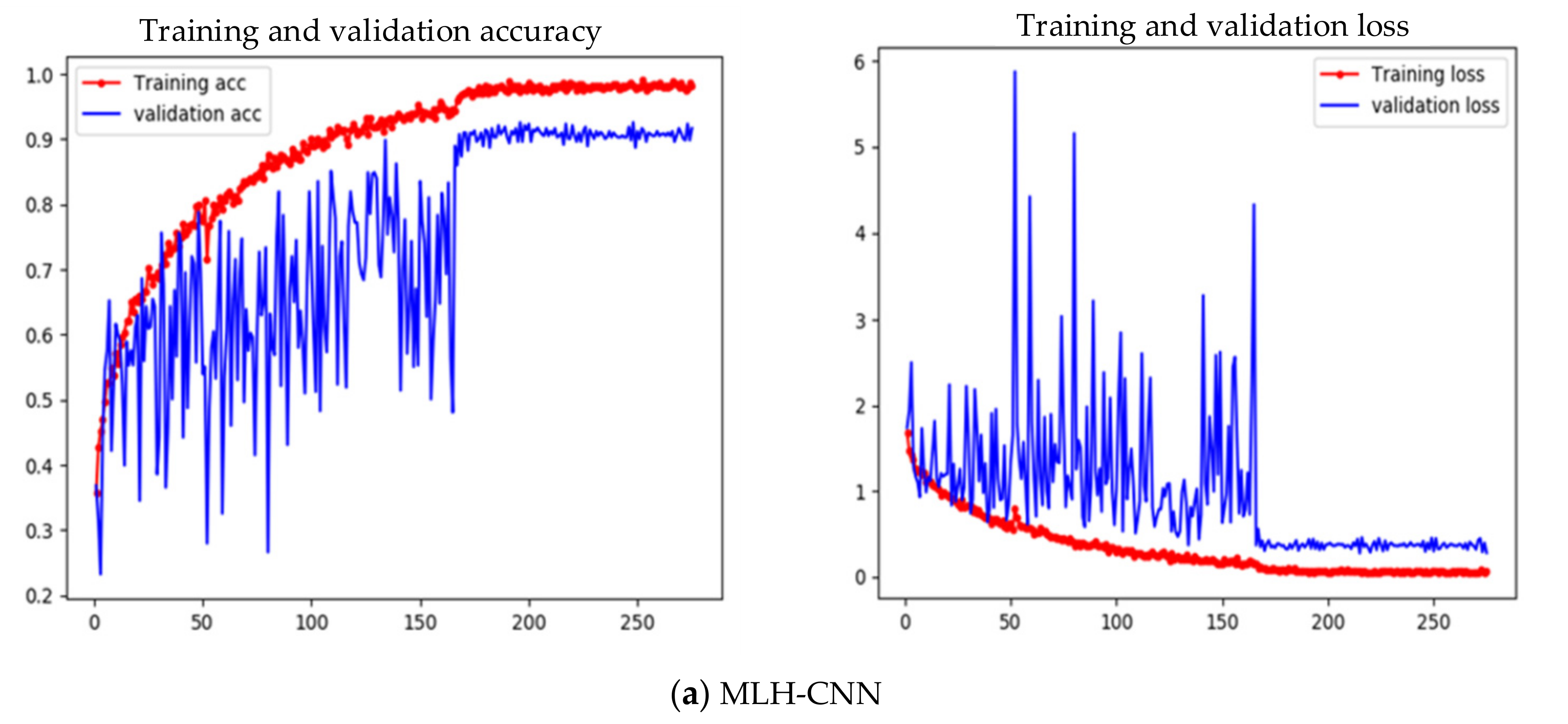
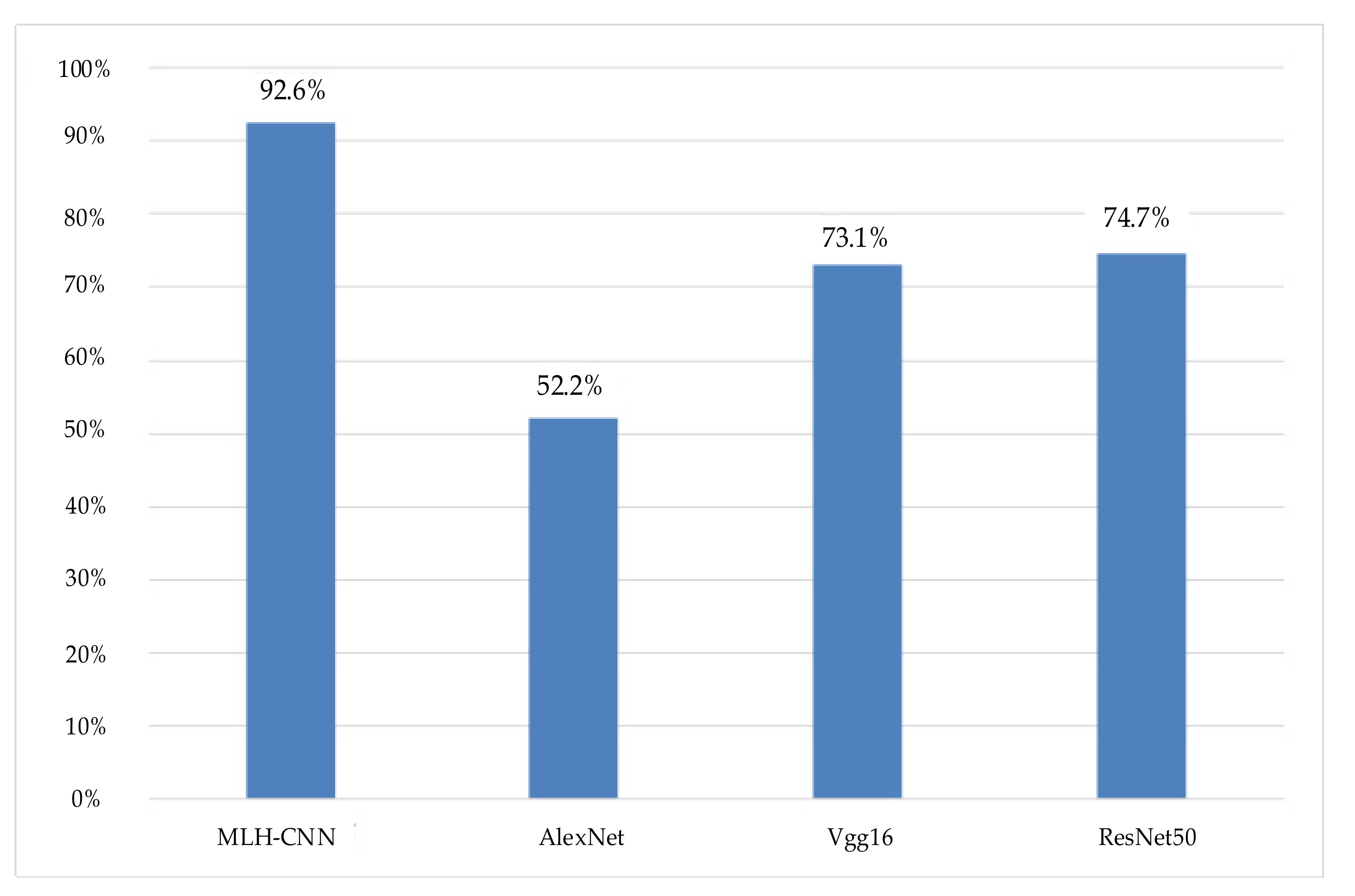
In order to verify the effectiveness of the proposed model, the training and verification curves of the whole training process of different methods, i.e., MLH-CNN, Vgg16, AlexNet, and ResNet50, are shown in Figure 6. It can be seen that the verification curve and loss curve of the four models fluctuate greatly in the early stage and kept oscillating until the later stage, which tended to be stable. Compared with other models, the proposed MLH-CNN is more stable in the later stage, and the classification accuracy is higher. A comparison of the classification accuracy of the four networks is shown in Figure 7. The accuracy of the proposed MLH-CNN is 92.6%, which is much higher than that of the other three networks.

4.3. Classification Index Analysis

In Figure 8, the precision, recall, and F1-score of each of the categories MLH-CNN, AlexNet, ResNet50, and Vgg16 are provided.
Figure 8 also lists the macro average value, micro average value, and weight average value of the waste classification. The micro average takes all the categories into account once to calculate the accuracy of category prediction. The macro average is used to consider each category separately, calculate the accuracy of each category separately, and finally to perform arithmetic averaging to obtain the accuracy of the dataset. It can be seen from the results in Figure 8 that the index of the trash category is relatively low, while the index of other categories is relatively high, which is closely related to the number and features of the training images. The reason for this is that the number of images in the trash category in the dataset is the least, and the features are very similar to other categories. Meanwhile, under the same conditions, the classification index of MLH-CNN is higher than other networks, which shows that the performance of MLH-CNN is good. The formula for recall, precision, and the F1-score are as follows:
P = T P T P + F P
r = T P T P + F N
F 1 = 2 r P 2 × T P + F P + F N
TP is the number of positive samples predicted to be positive samples. FN is the number of positive samples predicted to be negative samples. FP is the number of negative samples predicted to be positive samples. TN is the number of negative samples predicted to be negative samples.

4.4. Confusion Matrix Analysis

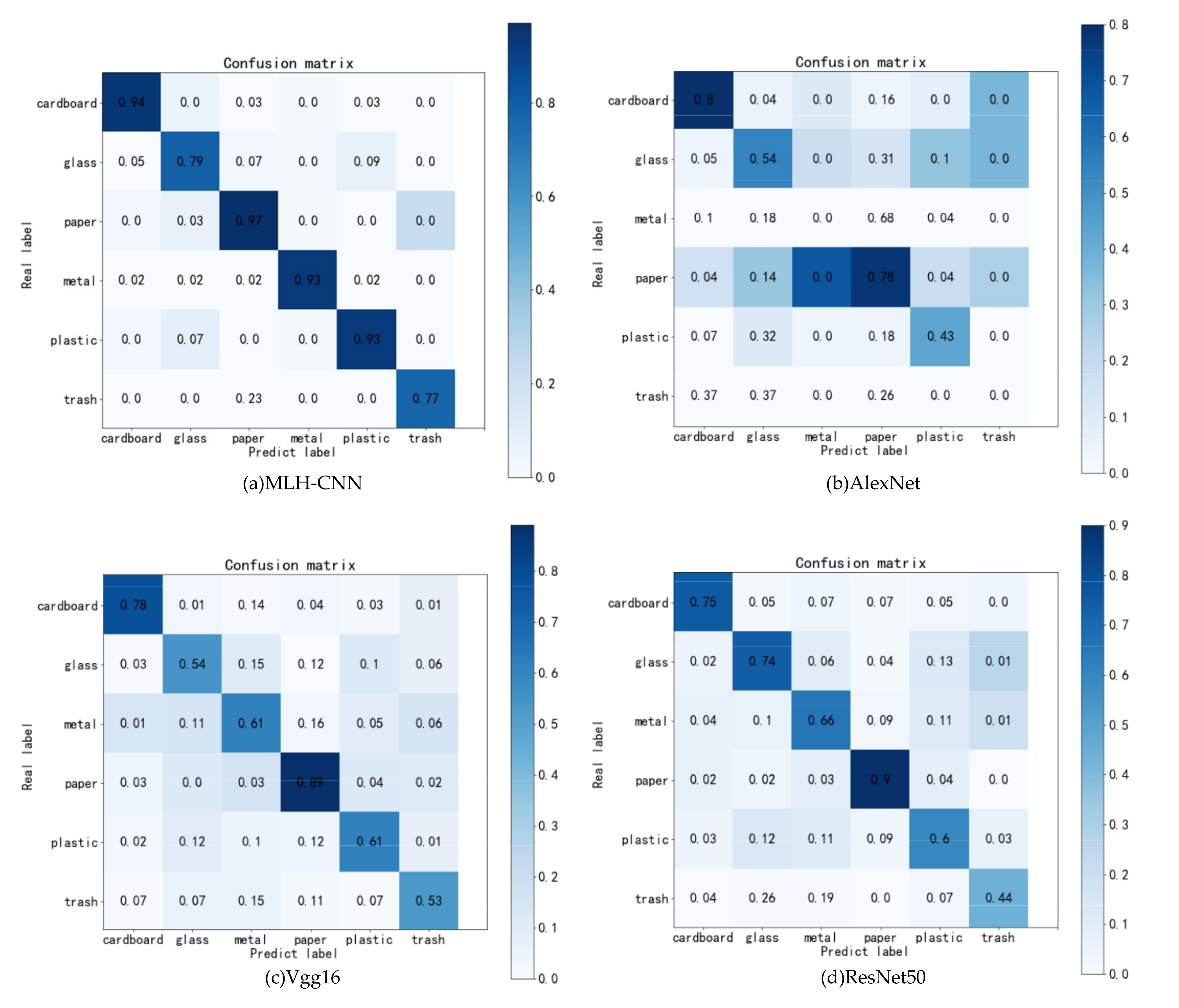
The confusion matrix can show the classification accuracy of each category, which is another effective index for evaluating the classification performance of a method. The confusion matrix of MLH-CNN, AlexNet, ResNet50, and Vgg16 on the TrashNet dataset is shown in Figure 9.
It can be seen in Figure 9 that the accuracy of the MLH-CNN prediction is concentrated on the diagonal, and the prediction accuracy of six categories are high, which is better than the other three classical networks, indicating that the model in this paper can provide a good classification performance.

4.5. Heat Map Analysis

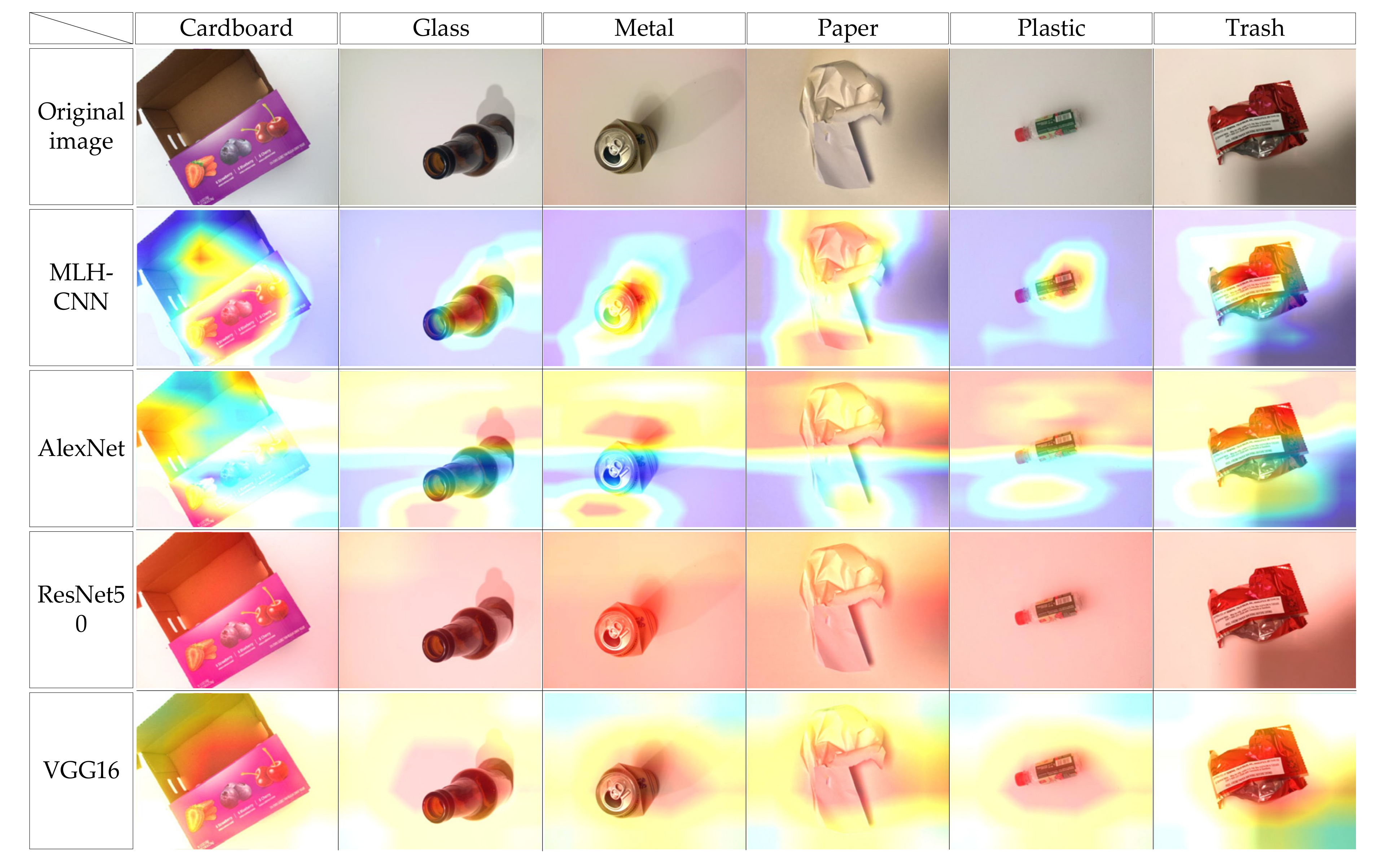
The heat maps of different images obtained by the MLH-CNN, AlexNet, ResNet50, and Vgg16 on the TrashNet dataset are shown in Figure 10. It can be seen that the heat maps obtained by the MLH-CNN method are all concentrated on the target regions. It is obvious that the proposed MLH-CNN method can focus on the main target and extract features effectively. For other network models such as AlexNet, ResNe50, and Vgg16, the region of interest in the heat maps also contain some image background, or even just image background. These will lead to poor feature extraction. Overall, the MLH-CNN method proposed in this paper has good feature extraction ability, which helps to provide good classification performance.

4.6. Analysis of Classification Results

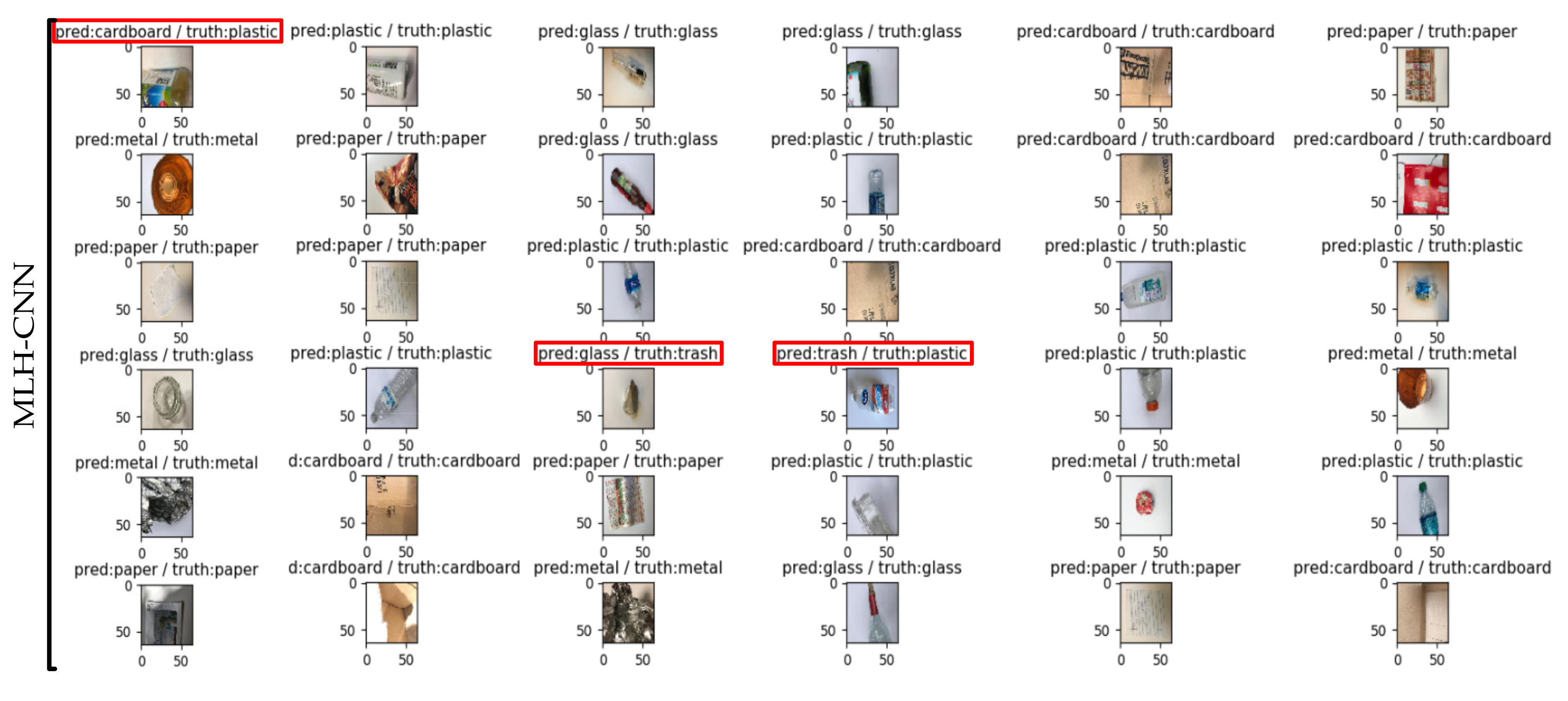
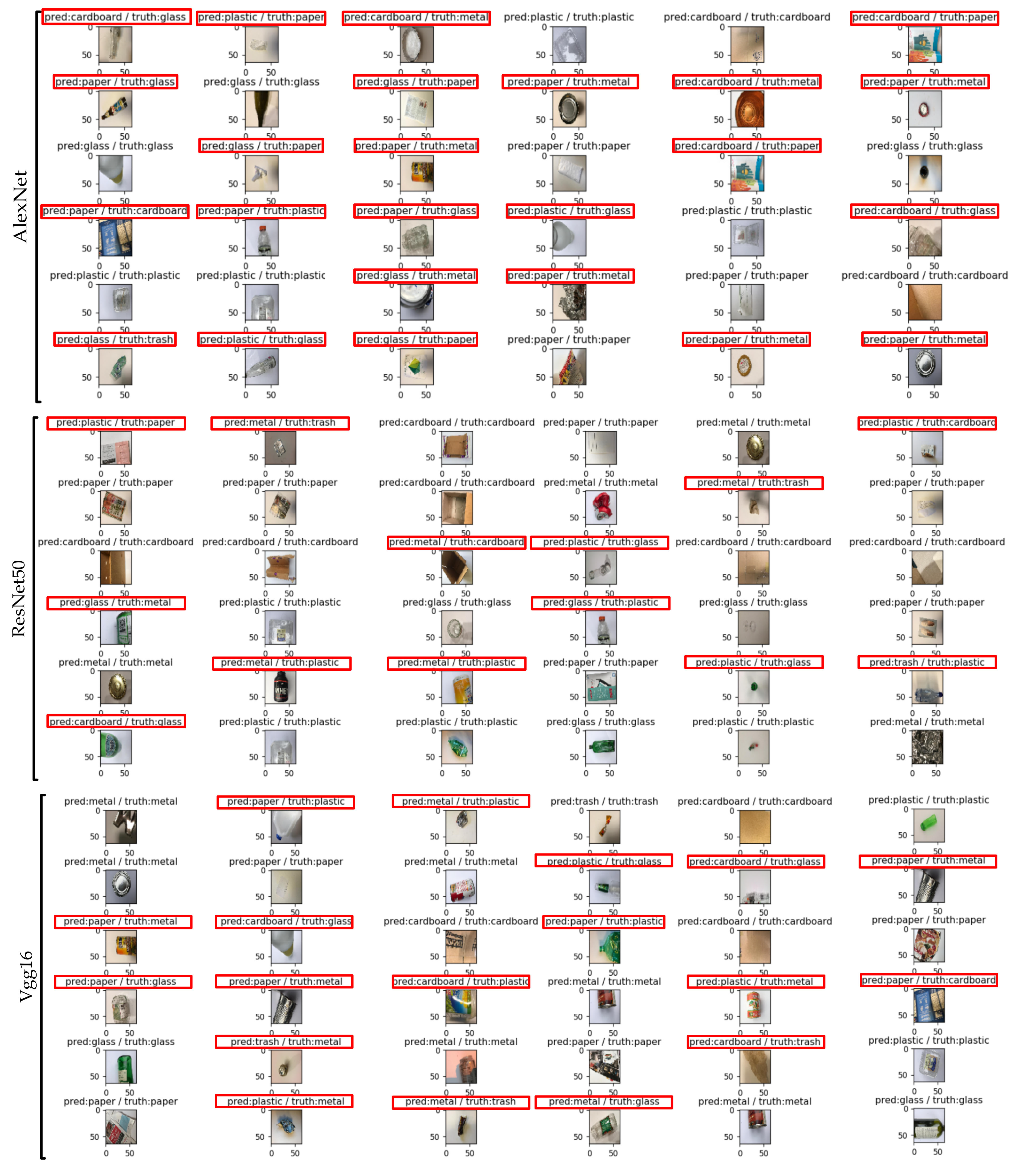
Figure 11 shows the test results of the MLH-CNN, AlexNet, ResNet50, and Vgg16 models on the TrashNet dataset. For this paper, 36 images were randomly selected from the test set; “pred” represents the sample label obtained from the test, “truth” represents the real sample label. The red box in Figure 11 indicates that the predicted sample label is inconsistent with the real sample label, which means that the classification is wrong. It can be seen from Figure 11 that MLH-CNN has the best classification result and the lowest error probability among the 36 randomly selected images of the test set, which indicates that the proposed model has good classification performance.

4.7. Partial Occlusion Test Experiment

In order to further verify the effectiveness of the proposed method, some occlusion tests were carried out on the TrashNet dataset. Firstly, the test set was divided into four parts. Figure 12a–d show some examples of partial occlusion at different positions. Then, the MLH-CNN, AlexNet, ResNet50, and Vgg16 were performed on the four different occlusion test sets. The classification results are listed in Table 5. These results show that the classification accuracy of the waste image declines in the case of occlusion. However, the classification accuracy of the proposed MLH-CNN is still far higher than that of the other three network models.

4.8. Comparison with Related Literature

With the same dataset, the proposed method is compared with other classification methods based on deep learning. The experimental results are listed in Table 6. Kennedy T et al. used the transfer learning method based on VGG19, which exploits pre-trained large-scale networks on a small amount of data using the transfer learning technology and achieved an 88.42% classification accuracy [20]. The work in [23] proposed a convolution neural network model constructed with the 50-layer residual network preprocessing (ResNet-50) as an extractor and used the support vector machine (SVM) to classify, achieving an 87% accuracy on a waste image set. The work in [27] proposed an improved model based on MobileNet and obtained a classification accuracy of 87.2%. After optimization and quantification, the accuracy reached 89.34%. The work in [30] took advantage of the classical deep learning models, trained a network with an Iception-ResNet model, and compared its classification performance with that of several convolution neural networks on a waste image dataset, finally achieving the best accuracy of 88.60%. Costa et al. studied different types of neural networks and classified the waste images into four categories, among which the accuracies obtained by the KNN, SVM, and RF pre-training model methods were 88.0%, 80.0%, and 85.0%, respectively [32]. Awe et al. used a Faster R-CNN [38] model with faster fine-tuning to classify the mixed waste images, and a 68.30% classification accuracy was achieved [39]. The work in [40] arranged the convolution neural network in parallel with various methods, and the best classification accuracy was 89.81%. In [41], the image processing used pre-trained deep convolutional networks with Single Shot Detectors (SSD) and MobileNetsV1. In [42], Vgg16, ResNet50, and Xception were pre-trained on ImageNet, and the highest classification rate was 88%. Most of the abovementioned methods used fine-tuning classical convolutional neural networks to classify waste images. Direct fine-tuning of classical convolutional neural networks has the disadvantage of having many network parameters and large computations. The proposed model achieved the best accuracy of 92.6% for waste classification. In addition, the proposed method had fewer parameters and a shorter iteration time. This means that the proposed method can provide a higher classification accuracy with lower complexity. Meanwhile, the classical convolution neural network based on fine-tuning is not suitable for the TrashNet dataset.

5. Conclusions

This paper analyzed the role of waste classification in daily life. With the increasing amount of waste discharge, intelligent waste classification is becoming more and more important. This paper discussed the waste classification methods in previous studies, which were mainly based on two methods, i.e., traditional methods and neural network methods. Finally, this paper proposed an effective waste classification method. The advantages of this method were proved by a large number of experiments. In this paper, a simple structure MLH-CNN model was proposed for waste image classification. The network structure of this method is similar to that of VggNet, but simpler. By changing the number of network modules and channels, the performance of the model could be improved. In the experiments, the proposed model was tested and evaluated by a variety of indicators such as precision, recall, and F1-score. Compared with the existing waste image classification methods based on the TrashNet dataset, the proposed MLH-CNN network has a simper structure and fewer parameters, and has better classification performance for the TrashNet dataset. The classification accuracy of the MLH-CNN model is up to 92.6%, which is 4.18% and 4.6% higher than that of some state-of-the-art methods.
Future work should focus on further improving the classification performance of the model. More importantly, further studies should aim to ensure classification accuracy, combined with the hardware system necessary to achieve intelligent and real-time waste classification.

Author Contributions

Conceptualization, C.T.; data curation, C.S. and C.T.; formal analysis, T.W.; methodology, C.S.; software, C.S. and C.T.; validation, C.T.; writing—original draft, C.T.; writing—review and editing, L.W. All authors have read and agreed to the published version of the manuscript.

Funding

This research was funded in part by the National Natural Science Foundation of China (41701479 and 62071084), in part by the Heilongjiang Science Foundation Project of China under Grant JQ2019F003, and in part by the Fundamental Research Funds in Heilongjiang Provincial Universities of China under Grant 135509136.

Institutional Review Board Statement

Not applicable.

Informed Consent Statement

Not applicable.

Data Availability Statement

Not applicable.

Acknowledgments

We would like to thank Mindy Yang and Gary Thung from Stanford University for providing the TrashNet dataset. And we would like to thank the handling editor and the anonymous reviewers for their careful reading and helpful comments.

Conflicts of Interest

The authors declare no conflict of interest.

References

  1. Zhang, S.; Forssberg, E. Intelligent Liberation and classification of electronic scrap. Powder Technol. 1999, 105, 295–301. [Google Scholar] [CrossRef]
  2. Lui, C.; Sharan, L.; Adelson, E.H.; Rosenholtz, R. Exploring features in a bayesian framework for material recognition. In Proceedings of the 2010 IEEE Computer Society Conference on Computer Vision and Pattern Recognition, San Francisco, CA, USA, 13–18 June 2010; pp. 239–246. [Google Scholar]
  3. Bai, J.; Lian, S.; Liu, Z.; Wang, K.; Liu, D. Deep learning based robot for automatically picking up garbage on the grass. IEEE Trans. Consum. Electron. 2018, 64, 382–389. [Google Scholar]
  4. Lin, I.; Loyola-González, O.; Monroy, R.; Medina-Pérez, M.A. A review of fuzzy and pattern-based approaches for class imbalance problems. Appl. Sci. 2021, 11, 6310. [Google Scholar] [CrossRef]
  5. Shangitova, Z.; Orazbayev, B.; Kurmangaziyeva, L.; Ospanova, T.; Tuleuova, R. Research and modeling of the process of sulfur production in the claus reactor using the method of artificial neural networks. J. Theor. Appl. Inf. Technol. 2021, 99, 2333–2343. [Google Scholar]
  6. Picón, A.; Ghita, O.; Whelan, P.F.; Iriondo, P.M. Fuzzy spectral and spatial feature integration for classification of nonferrous materials in hyperspectral data. IEEE Trans. Ind. Inform. 2009, 5, 483–494. [Google Scholar] [CrossRef]
  7. Shylo, S.; Harmer, S.W. Millimeter-wave imaging for recycled paper classification. IEEE Sens. J. 2016, 16, 2361–2366. [Google Scholar] [CrossRef]
  8. Rutqvist, D.; Kleyko, D.; Blomstedt, F. An automated machine learning approach for smart waste management systems. IEEE Trans. Ind. Inform. 2020, 16, 384–392. [Google Scholar] [CrossRef]
  9. Zheng, J.; Xu, M.; Cai, M.; Wang, Z.; Yang, M. Modeling group behavior to study innovation diffusion based on cognition and network: An analysis for garbage classification system in Shanghai, China. Int. J. Environ. Res. Public Health 2019, 16, 3349. [Google Scholar] [CrossRef] [Green Version]
  10. Chu, Y.; Huang, C.; Xie, X.; Tan, B.; Kamal, S.; Xiong, X. Multilayer hybrid deep-learning method for waste classification and recycling. Comput. Intell. Neurosci. 2018, 1–9. [Google Scholar] [CrossRef] [Green Version]
  11. Donovan, J. Auto-Trash Sorts Waste Automatically at the TechCrunch Disrupt Hackathon; Techcrunch Disrupt Hackaton: San Francisco, CA, USA, 2018. [Google Scholar]
  12. Batinić, B.; Vukmirović, S.; Vujić, G.; Stanisavljević, N.; Ubavin, D.; Vukmirović, G. Using ANN model to determine future waste characteristics in order to achieve specific waste management targets-case study of Serbia. J. Sci. Ind. Res. 2011, 70, 513–518. [Google Scholar]
  13. Krizhevsky, A.; Sutskever, I.; Hinton, G.E. Imagenet classification with deep convolutional neural networks. Adv. Neural Inf. Process. Syst. 2012, 25, 1097–1105. [Google Scholar] [CrossRef]
  14. O’Toole, M.D.; Karimian, N.; Peyton, A.J. Classification of nonferrous metals using magnetic induction spectroscopy. IEEE Trans. Ind. Inform. 2018, 14, 3477–3485. [Google Scholar] [CrossRef] [Green Version]
  15. Zhao, D.-E.; Wu, R.; Zhao, B.-G.; Chen, Y.-Y. Research on waste classification and recognition based on hyperspectral imaging technology. Spectrosc. Spectr. Anal. 2019, 39, 917–922. [Google Scholar]
  16. Yusoff, S.H.; Mahat, S.; Midi, N.S.; Mohamad, S.Y.; Zaini, S.A. Classification of different types of metal from recyclable household waste for automatic waste separation system. Bull. Electr. Eng. Inform. 2019, 8, 488–498. [Google Scholar] [CrossRef]
  17. Zeng, D.; Zhang, S.; Chen, F.; Wang, Y. Multi-scale CNN based garbage detection of airborne hyperspectral data. IEEE Access 2019, 7, 104514–104527. [Google Scholar] [CrossRef]
  18. Roh, S.B.; Oh, S.K.; Pedrycz, W. Identification of black plastics based on fuzzy rbf neural networks: Focused on data preprocessing techniques through fourier transform infrared radiation. IEEE Trans. Ind. Inform. 2018, 14, 1802–1813. [Google Scholar] [CrossRef]
  19. Simonyan, K.; Zisserman, A. Very deep convolutional networks for large-scale image recognition. arXiv 2014, arXiv:1409.1556. [Google Scholar]
  20. Kennedy, T. OscarNet: Using transfer learning to classify disposable waste. In CS230 Report: Deep Learning; Stanford University: Stanford, CA, USA, 2018. [Google Scholar]
  21. Veit, A.; Wilber, M.J.; Belongie, S. residual networks behave like ensembles of relatively shallow networks. Adv. Neural Inf. Process. Syst. 2016, 29, 550–558. [Google Scholar]
  22. Kadyrova, N.O.; Pavlova, L.V. Comparative efficiency of algorithms based on support vector machines for binary classification. Biophysics 2015, 60, 13–24. [Google Scholar] [CrossRef]
  23. OAdedeji, O.; Wang, Z. Intelligent waste classification system using deep learning convolutional neural network. Procedia Manuf. 2019, 35, 607–612. [Google Scholar] [CrossRef]
  24. Li, B.; Wu, W.; Wang, Q.; Zhang, F.; Xing, J.; Yan, J. SiamRPN++: Evolution of siamese visual tracking with very deep networks. In Proceedings of the 2019 IEEE/CVF Conference on Computer Vision and Pattern Recognition (CVPR), Long Beach, CA, USA, 15–20 June 2019; pp. 4277–4286. [Google Scholar]
  25. Zhihong, C.; Hebin, Z.; Yanbo, W.; Binyan, L.; Yu, L. A vision-based robotic grasping system using deep learning for garbage sorting2017. In Proceedings of the 36th Chinese Control Conference (CCC), Dalian, China, 26–28 July 2017. [Google Scholar]
  26. Howard, A.G.; Zhu, M.; Chen, B.; Kalenichenko, D.; Wang, W.; Weyand, T.; Adam, H. Mobilenets: Efficient convolutional neural networks for mobile vision applications. arXiv 2017, arXiv:1704.04861. [Google Scholar]
  27. Rabano, S.L.; Cabatuan, M.K.; Sybingco, E.; Dadios, E.P.; Calilung, E.J. Common garbage classification using mobilenet. In Proceedings of the 2018 IEEE 10th International Conference on Humanoid, Nanotechnology, Information Technology, Communication and Control, Environment and Management (HNICEM), Baguio City, Philippines, 29 November–2 December 2018; pp. 1–4. [Google Scholar]
  28. He, K.; Zhang, X.; Ren, S.; Sun, J. Deep residual learning for image recognition. In Proceedings of the IEEE Conference on Computer Vision and Pattern Recognition, Las Vegas, NV, USA, 27–30 June 2016; pp. 770–778. [Google Scholar]
  29. Szegedy, C.; Liu, W.; Jia, Y.; Sermanet, P.; Reed, S.; Anguelov, D.; Rabinovich, A. Going deeper with convolutions. In Proceedings of the IEEE Conference on Computer Vision and Pattern Recognition (CVPR), Boston, MA, USA, 7–12 June 2015; pp. 1–9. [Google Scholar]
  30. Ruiz, V.; Sánchez, Á.; Vélez, J.F.; Raducanu, B. Automatic image-based waste classification. In International Work-Conference on the Interplay between Natural and Artificial Computation; Springer: Cham, Switzerland, 2019; Volume 11487, pp. 422–431. [Google Scholar]
  31. Abeywickrama, T.; Cheema, M.A.; Taniar, D. K-Nearest neighbors on road networks: A journey in experimentation and in-memory implementation. Proc. VLDB Endow. 2016, 9, 492–503. [Google Scholar] [CrossRef]
  32. Costa, B.S.; Bernardes, A.C.; Pereira, J.V.; Zampa, V.H.; Pereira, V.A.; Matos, G.F.; Silva, A.F. Artificial intelligence in automated sorting in trash recycling. In Anais do XV Encontro Nacional de Inteligência Artificial e Computacional; SBC: Brasilia, Brazil, 2018; pp. 198–205. [Google Scholar]
  33. Miao, N.; Song, Y.; Zhou, H.; Li, L. Do you have the right scissors? Tailoring pre-trained language models via monte-carlo methods. In Proceedings of the 58th Annual Meeting of the Association for Computational Linguistics, Washington, DC, USA, 13 July 2020; pp. 3436–3441. [Google Scholar]
  34. Ioffe, S.; Szegedy, C. Batch Normalization: Accelerating deep network training by reducing internal covariate shift. In Proceedings of the International Conference on Machine Learning, Lille, France, 6–11 July 2015; pp. 448–456. [Google Scholar]
  35. Kingma, D.P.; Ba, J. Adam: A method for stochastic optimization. arXiv 2014, arXiv:1412.6980. [Google Scholar]
  36. Robbins, H.; Monro, S. A stochastic approximation method. Ann. Math. Stat. 1951, 22, 400–407. [Google Scholar] [CrossRef]
  37. Yang, M.; Thung, G. Classification of trash for recyclability status. In CS229 Project Report; Publisher Name: San Francisco, CA, USA, 2016. [Google Scholar]
  38. Ren, S.; He, K.; Girshick, R.; Sun, J. Faster R-CNN: Towards real-time object detection with region proposal networks. In Proceedings of the IEEE Transactions on Pattern Analysis and Machine Intelligence, Las Vegas, NV, USA, 27–30 June 2016; Volume 39, pp. 1137–1149. [Google Scholar]
  39. Awe, O.; Mengistu, R.; Sreedhar, V. Smart trash net: Waste localization and classification. arXiv 2017, preprint. [Google Scholar]
  40. Satvilkar, M. Image Based Trash Classification using Machine Learning Algorithms for Recyclability Status. Master’s Thesis, National College of Ireland, Dublin, Ireland, 2018. [Google Scholar]
  41. Melinte, D.O.; Dumitriu, D.; Mărgăritescu, M.; Ancuţa, P.N. Deep Learning Computer Vision for Sorting and Size Determination of Municipal Waste; Springer: Cham, Switzerland, 2020; Volume 85, pp. 142–152. [Google Scholar]
  42. Endah, S.N.; Shiddiq, I.N. Xception architecture transfer learning for waste classification. In Proceedings of the 2020 4th International Conference on Informatics and Computational Sciences (ICICoS), Semarang, Indonesia, 10–11 November 2020; pp. 1–4. [Google Scholar] [CrossRef]
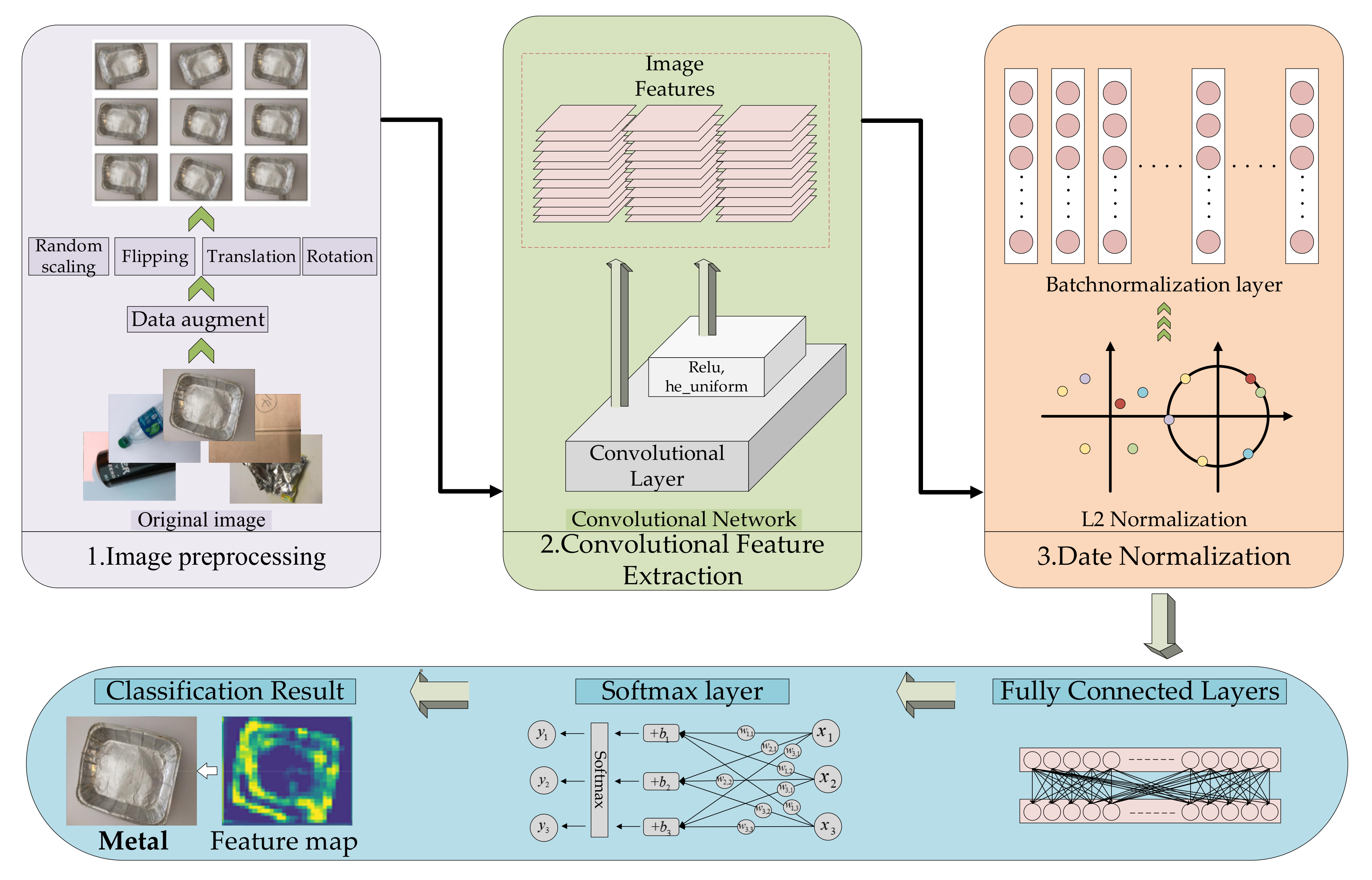
Figure 1. The overall process of the proposed waste classification method.
Applsci 11 08572 g001
Figure 2. The structure of the proposed modules.
Applsci 11 08572 g002
Figure 3. The final network structure adopted in this paper.
Applsci 11 08572 g003
Figure 4. Comparison of the accuracy of the optimizers Adam, SGD, and SGDM + Nesterov.
Applsci 11 08572 g004
Figure 5. Some images from the TrashNet dataset. (a) Cardboard sample, (b) Glass sample, (c) Metal sample, (d) Paper sample, (e) Plastic sample, (f) Trash sample.
Applsci 11 08572 g005
Figure 6. The training and verification results of the proposed method. (a) MLH-CNN training and validation curve, (b) AlexNet training and validation curve, (c) Vgg16 training and validation curve, (d) ResNet50 training and validation curve.
Applsci 11 08572 g006aApplsci 11 08572 g006b
Figure 7. The classification accuracy of the four networks.
Applsci 11 08572 g007
Figure 8. The results of evaluation indexes of the proposed method.
Applsci 11 08572 g008aApplsci 11 08572 g008b
Figure 9. The confusion matrix of different methods.
Applsci 11 08572 g009
Figure 10. Comparison of heat map results of different methods.
Applsci 11 08572 g010
Figure 11. Classification results of the TrashNet set.
Applsci 11 08572 g011aApplsci 11 08572 g011b
Figure 12. Some examples of occlusion in the TrashNet test set. (a) The lower right corner is occluded; (b) the lower left corner is occluded; (c) the top left corner is occluded; (d) the top right corner is occluded.
Applsci 11 08572 g012
Table 1. The structures of the initial network model and some of its improved versions.
The Proposed MethodStructureAccuracyOne Iteration Time
The initial modelA module made up of the basic modules, shown in Figure 286.20%114 ms/step
The first improved modelThe three modules are used for mixing87.20%189 ms/step
The second improved modelThe three modules and one basic module are used for mixing89.70%201 ms/step
The third improved modelThe four modules are used for mixing92.60%223 ms/step
The fourth improved modelThe five modules are used for mixing88.50%240 ms/step
Table 2. Accuracy and time consumption of the optimizers Adam, SGD, and SGDM.
OptimizerAccuracyTime One Iteration Takes
Adam90.2%235 ms/step
SGD89.7%225 ms/step
SGDM + Nesterov92.6%223 ms/step
Table 3. Hyper-parameter configuration of the network.
Optimizer (Momentum Parameter)SGDM + Nesterov (0.9)
Learning rate0.1
Patient value30
Batch size32
Batch NormalizationMomentum = 0.99, epsilon = 0.001
Table 4. Number of samples for each category in the training set and test set.
CardboardGlassPaperMetalPlasticTrash
Train number323401476328386110
Test number80100118829627
Table 5. Comparison of classification accuracy of different occlusion tests.
MLH-CNNResNet50Vgg16AlexNet
The lower right corner is blocked83.44%67.59%65.01%45.92%
The lower left corner is blocked84.75%71.37%69.38%46.52%
The top left corner is blocked83.01%71.77%62.82%46.92%
The top right corner is blocked79.96%71.77%70.58%46.9%
Table 6. Comparison of the results of the proposed method and other classification methods.
DatasetMethodYearParametersAccuracyGain
TrashNetOscarNet (based on VGG19 pretrained) [20]201813,957,024088.42%4.18%
Augmented data to train R-CNN [39]2017--68.30%24.3%
Ref. [23]201922,515,07887.00%5.6%
Ref. [30] with Inception-ResNet201929,042,34488.66%3.94%
Ref. [33] with KNN2018--88.00%4.6%
Ref. [33] with SVM2018--80.00%12.6%
Ref. [33] with RF2018--85.00%7.6%
Ref. [27] with MobileNet201842,000,00089.34%3.26%
Ref. [40] with CNN2018--89.81%2.79%
Ref. [41]202029,000,00088.42%4.18%
Ref. [42]202020,875,24788%4.6%
Ours (MLH-CNN)--1,709,92692.60%--
Publisher’s Note: MDPI stays neutral with regard to jurisdictional claims in published maps and institutional affiliations.