Article

Consecutive Independence and Correlation Transform for Multimodal Data Fusion: Discovery of One-to-Many Associations in Structural and Functional Imaging Data

by
Chunying Jia
1,*,
Mohammad Abu Baker Siddique Akhonda
1,
Yuri Levin-Schwartz
2,
Qunfang Long
1,
Vince D. Calhoun
3 and
Tülay Adali
1
1
Department of Computer Science and Electrical Engineering, University of Maryland Baltimore County, Baltimore, MD 21250, USA
2
Icahn School of Medicine at Mount Sinai, New York, NY 10029, USA
3
Tri-Institutional Center for Translational Research in Neuroimaging and Data Science (TReNDS), Georgia State University, Georgia Institute of Technology, and Emory University, Atlanta, GA 30030, USA
*
Author to whom correspondence should be addressed.
Appl. Sci. 2021, 11(18), 8382; https://doi.org/10.3390/app11188382
Submission received: 19 July 2021 / Revised: 31 August 2021 / Accepted: 4 September 2021 / Published: 9 September 2021
(This article belongs to the Special Issue Advances in Biomedical Image Processing and Analysis)

Abstract

:
Brain signals can be measured using multiple imaging modalities, such as magnetic resonance imaging (MRI)-based techniques. Different modalities convey distinct yet complementary information; thus, their joint analyses can provide valuable insight into how the brain functions in both healthy and diseased conditions. Data-driven approaches have proven most useful for multimodal fusion as they minimize assumptions imposed on the data, and there are a number of methods that have been developed to uncover relationships across modalities. However, none of these methods, to the best of our knowledge, can discover “one-to-many associations”, meaning one component from one modality is linked with more than one component from another modality. However, such “one-to-many associations” are likely to exist, since the same brain region can be involved in multiple neurological processes. Additionally, most existing data fusion methods require the signal subspace order to be identical for all modalities—a severe restriction for real-world data of different modalities. Here, we propose a new fusion technique—the consecutive independence and correlation transform (C-ICT) model—which successively performs independent component analysis and independent vector analysis and is uniquely flexible in terms of the number of datasets, signal subspace order, and the opportunity to find “one-to-many associations”. We apply C-ICT to fuse diffusion MRI, structural MRI, and functional MRI datasets collected from healthy controls (HCs) and patients with schizophrenia (SZs). We identify six interpretable triplets of components, each of which consists of three associated components from the three modalities. Besides, components from these triplets that show significant group differences between the HCs and SZs are identified, which could be seen as putative biomarkers in schizophrenia.

1. Introduction

Imaging and electrophysiological techniques that effectively quantify brain functions and structures facilitate our understanding of human brain function in healthy populations and those suffering from neuropsychiatric diseases such as schizophrenia [1,2,3,4]. For example, the magnetic resonance imaging (MRI)-based methods diffusion MRI (dMRI) [5], structural MRI (sMRI) [6], and functional MRI (fMRI) [7] are three brain-imaging modalities that convey information about structural connectivity, regional brain volume, and functional activity/connectivity, respectively. DMRI estimates white matter (WM) connectivity based on the differential diffusion rates of water molecules in different brain tissues. SMRI provides information about the morphology of brain tissues including WM, grey matter (GM), and cerebrospinal fluid (CSF). FMRI detects neuronal activations by measuring the blood oxygenation level-dependent response in the brain. Each of these three imaging techniques reveals different yet complementary information about brain structures or activities. Because of the intrinsic relationships between the structure and activity of the brain, multiple associations between these modalities are expected. This motivates the increasing popularity of collecting data from the same subjects using multiple modalities [8,9]. A joint analysis of such multimodal data should be useful for finding multiple associations across modalities, revealing the mechanisms of brain functions and potentially improving the predictive power to diagnose diseases compared with unimodal analyses. Data fusion is concerned with the simultaneous analyses of such joint datasets to obtain a global view of a problem under study or a system under observation by leveraging the information that is available across multiple datasets so that further analyses (e.g., detection, classification) can be improved [10,11,12].
However, since the relationships between different modalities are largely unknown, data-driven methods are particularly attractive. In this regard, data-driven methods based on blind source separation (BSS) have proven to be particularly useful for data fusion due to their ability to decompose the observed data into a set of latent variables, also known as components, through a simple generative model [13,14,15,16]. The components obtained from different datasets separately or jointly through the BSS techniques could be used to reveal potential relationships between different datasets. For example, components obtained from the datasets of sMRI and fMRI through the BSS techniques show locations and intensities of separated source signals in the brain (i.e., spatial maps) and allow us to find how the brain activities (fMRI) are related to the brain structures (sMRI). Importantly, due to the existence of systematic noise and interference in the real-world data, performing data fusion in the signal subspace with proper numbers of components (i.e., orders of signal subspace) effectively reduces the noise and interference and thus enables a better generalization ability.
Among various BSS techniques, independent component analysis (ICA) [17] and canonical correlation analysis (CCA) [18,19], as well as their extensions to multiple datasets—independent vector analysis (IVA) [20,21] and multi-set CCA (mCCA) [22,23]—have proven to be especially useful for data fusion. With a linear mixing model and the assumption of statistical independence, ICA decomposes observations into maximally independent components (ICs). IVA generalizes ICA to multiple data sets and utilizes the statistical dependence across different data sets to achieve a powerful solution for data fusion [20,24]. CCA and mCCA, on the other hand, make use of second-order statistics (correlation), and it can be shown that IVA generalizes both [21].
A number of models based on ICA, IVA, CCA, and mCCA have been developed for data fusion, such as joint ICA (jICA) [25], mCCA + jICA [26], and transposed IVA (tIVA) [15,27]. JICA concatenates all the datasets together and then performs ICA on the joint dataset for data fusion. The jICA model assumes a common mixing matrix and order as well as equal contributions across all datasets—a set of strong constraints, especially for more than two modalities. For mCCA + jICA, the use of mCCA in the first stage relaxes the strong assumptions of identical mixing matrices; however, a common order for the different modalities is still needed. TIVA also requires a common order in different modalities and a significantly large number of subjects for enough statistical power, which in a large number of cases is not feasible in current experimental settings. Collectively, none of these methods are flexible in terms of dealing with different orders and finding “one-to-many associations” in real-world data. However, firstly, due to the disparate measurements in different modalities, the order of the signal subspace is very likely to be different between modalities [28,29]. Secondly, one component in one modality might be associated with multiple components in other modalities because of the intrinsic relationships between modalities. For instance, the same WM connects multiple regions of the GM; thus, “one-to-many associations” between dMRI and sMRI datasets are expected. Besides, the fusion of more than two modalities of brain imaging data is expected to further facilitate exploiting joint information beyond pair-wise associations; nonetheless, most data fusion methods have been implemented to find multiple associations between only two modalities [26]. Therefore, a new framework for multi-modal data fusion is needed that is fully flexible in terms of the number of datasets combined, allowing for different orders across modalities and the discovery of “one-to-many associations”.
In this study, we propose a fully flexible data fusion framework, consecutive independence and correlation transform (C-ICT), to jointly analyze more than two datasets. By successively performing ICA and IVA, C-ICT exploits the strengths of ICA and IVA for the joint analysis of multimodal data. First, ICA is performed on individual datasets separately to obtain maximally independent components and corresponding subject profile matrices (first-level mixing matrices). Second, meaningful ICs and the corresponding subject profiles are selected for further analysis. Third, IVA with a multivariate Gaussian model (IVA-G) [30] is performed on the subject profile matrices of different datasets to obtain the source component vectors (SCVs) and the second-level mixing matrices. SCVs that show significant pair-wise correlations are chosen for further analysis. Finally, we trace back to the ICs in the first stage based on subject profiles with the highest contribution to the correlated SCVs and identify them as associated components across different modalities. Thus, C-ICT is fully flexible in terms of the number of datasets combined, the numbers of orders of the signal subspace for each dataset, and the discovery of “one-to-many associations”, and builds on the related concept we introduced in [28] for only two datasets.
We apply this new method to the fusion of data from three brain-imaging modalities (dMRI, sMRI, and resting-state fMRI) to search for possible multiple associations across these datasets. The data were collected from 86 healthy controls (HCs) and 76 patients with schizophrenia (SZs). Due to the intrinsic differences of these three data modalities, the choice of different orders for the three datasets is critical, which is accommodated by C-ICT. Importantly, prior to the IVA stage, we implemented an additional step to remove artifact components, as these might have contaminated the inherent associations across the modalities—a step which we note to be critical to the success of the method. It is shown that C-ICT successfully discovers multiple associations among the three modalities, including “one-to-many associations”. First, multiple associations successfully discovered in this study are consistent with existing structure–function networks. Second, among the three modalities in each triplet, dMRI and sMRI components show stronger associations than other modality pairs (dMRI and fMRI; sMRI and fMRI), which is consistent with the fact that the GM structure and WM structure are more intrinsically related than other pairs. These results demonstrate that our proposed C-ICT method is a flexible and powerful tool to find associative relationships across related data of different modalities.

2. Materials and Methods

2.1. Human Brain Data

2.1.1. Data Acquisition

The data used in this study were dMRI, sMRI, and resting-state fMRI data from the Center of Biomedical Research Excellence (COBRE), available from the Collaborative Informatics and Neuroimaging Suite data exchange repository [31,32] (coins.trendscenter.org/, accessed on 8 October 2018). All the three datasets include the same 86 HCs (average age: 36.6 ± 12.1 years) and 76 SZs (average age: 36.9 ± 13.5 years). All patients completed the Structured Clinical Interview for DSM-IV Axis I Disorders (SCID [33]) for diagnostic confirmation (consensus was reached by two research psychiatrists using the SCID-DSM-IV-TR, patient version) and evaluation for co-morbidities [34]. The battery of cognitive performance tests used was the MATRICS (Measurement and Treatment Research to Improve Cognition in Schizophrenia) Cognitive Battery, including seven cognitive domains: speed of processing, attention/vigilance, working memory, verbal learning, visual learning, reasoning, and problem solving, and social cognition. We performed two-sample t-tests on these cognitive scores from the HC and SZ subjects. Compared with healthy controls, SZs had a significantly lower cognitive performance on all domains, supporting the findings that patients diagnosed with schizophrenia have an abnormal cognitive function.
DMRI data were collected along the anterior commissure–posterior commissure (AC–PC) line throughout the whole brain with a field of view (FOV) of 256 × 256   mm 2 , a 128 × 128 matrix, 72 slices with a slice thickness of 2 mm (2 mm isotropic resolution), a number of excitations (NEX) of 1, echo time (TE) of 84 ms, and repetition time (TR) of 9000 ms. A multiple-channel radio-frequency (RF) coil was used, with GeneRalized Autocalibrating Partial Parallel Acquisition (GRAPPA) (X2), with 30 gradient directions with a b of 800 s/ mm 2 . The b = 0 experiment was repeated five times [35] and equally interspersed between the 30 gradient directions. The total scan time was about 6 min. This procedure was repeated twice to increase the signal-to-noise ratio (SNR).
For the sMRI data collection, the echo planar imaging (EPI) slices were collected in a sequential ascending order on a Siemens 3 T TIM Trio scanner using a 12-channel head coil. A sagittal gradient echo scout image through the mid-line was obtained to prescribe oblique axial image slices that were parallel to the AC–PC line. To minimize the susceptibility artifact in the orbitofrontal area, oblique slices were used [36]. High-resolution T1-weighted images were acquired with a five-echo multi-echo magnetization-prepared rapid gradient-echo (MP-RAGE) sequence (TE = 1.64, 3.5, 5.36, 7.22, 9.08 ms, TR = 2.53 s, TI (inversion time) = 1.2 s, flip angle = 7 , NEX = 1, slice thickness = 1 mm, FOV = 256 mm, resolution = 256 × 256 ) for region of interest analyses and spatial normalization.
The resting-state fMRI data were acquired using a conventional single-shot, gradient echo echo-planar pulse sequence with lipid suppression (TE = 29 ms; TR = 2000 ms; flip angle = 75 ; FOV = 240 mm; matrix size = 64 × 64 ; 33 slices; voxel size: 3.75 × 3.75 × 4.55   mm 3 ). The first image of each run was removed to eliminate T1 equilibrium effects [37].The participants were instructed to keep their eyes open during the scan and stare passively at a central fixation cross for about 5 min.

2.1.2. Data Preprocessing and Feature Extraction

Neuroimaging data are usually high-dimensional, with each modality having different properties and dimensions. For example, sMRI data contain spatial information with a high spatial resolution but contain no temporal information. FMRI data convey both temporal information and spatial information, but with a lower spatial resolution. To jointly analyze different datasets in a common subspace, it is important to reduce data of each modality down to a single feature for each subject, a multivariate lower-dimensional representation of the data, and collect the features from all subjects together in a single dataset [13,15]. Such a reduction enables the datasets from all modalities to share a common dimension—i.e., the number of subjects—which provides a natural connection across different data types.
The dMRI data we used were preprocessed using the FMRIB Software Library (https://fsl.fmrib.ox.ac.uk/fsl/fslwiki/, accessed on 8 October 2018). We carried out the preprocessing steps as follows: (1) we identified and removed excessive motion or vibration artifacts through a quality check with any gradient directions; (2) we corrected motion and eddy currents; (3) we corrected gradient directions for any image rotation caused by the previous motion correction step; and (4) we calculated the diffusion tensor and then derived the scalar measure—fractional anisotropy (FA)—from the tensor. The FA, a measurement of WM integrity, was calculated as the fraction of total diffusion that can be attributed to anisotropic diffusion. A higher value of FA corresponds to more consistent diffusion orientation and thus more integrity of WM [38]. The FA maps were smoothed with an 8 mm full-width half-maximum (FWHM) Gaussian filter and then used as the feature for dMRI data.
Using the unified segmentation method in Statistical Parametric Mapping (SPM8) (http://www.fil.ion.ucl.ac.uk/spm, accessed on 8 October 2018), the sMRI data were (1) normalized to the Montreal Neurological Institute (MNI) space; (2) resliced to 3 × 3 × 3   mm 3 ; and (3) segmented into GM, WM, and CSF images. The segmented GM images were then smoothed with an 8 mm FWHM Gaussian filter. We further detected subject outliers using the spatial Pearson correlation with a template image to ensure that all images of subjects were properly segmented [39]. The GM images were used as the feature for sMRI data.
The fMRI data were preprocessed using an automated analysis pipeline [40] carried out in SPM8. The pipeline consisted of (1) aligning all the images with the first image as the reference using INRIalign approach [41] to correct minor motions of the subject; (2) correcting for time differences between the slices using the middle slice as the reference; and (3) spatial normalization to MNI space, including reslicing to 3 × 3 × 3   mm 3 , resulting in 53 × 63 × 46 voxels. We then regressed out six motion parameters, WM, and CSF signals to further denoise the data. Data were then spatially smoothed with an 8 mm FWHM Gaussian filter. We estimated the fractional amplitude of low-frequency fluctuation (fALFF) [42], which is an effective approach to represent brain activity with high sensitivity and specificity that has been used in a large array of studies [43,44,45,46,47,48]. The fALFF is calculated as the ratio of the power spectrum of low frequency (0.0–0.08 Hz) to that of the whole detectable frequency range (0–0.25 Hz) [49]. The fALFF maps were then used as the feature for fMRI in this study.
For each modality, based on its own extracted feature, a two-dimensional matrix—feature dataset—was formed by concatenating the features across all subjects. These feature datasets from different modalities have a common dimension—the number of subjects—thus enabling the discovery of associations among different modalities through the variations across subjects.

2.2. Background

2.2.1. ICA

ICA is a statistical method that seeks to recover latent sources from a set of observed data with the assumption that the latent sources are statistically independent of one another [50]. Since it places few assumptions on data, ICA has been widely used in brain imaging studies [51,52,53,54].
Given a feature dataset X R M × V comprised of M subjects and V samples (e.g., voxels), the generative model for noiseless ICA can be written as
X = A S ,
where A R M × M is a full rank square mixing matrix and S R M × V is the latent sources. The goal of ICA is to estimate a demixing matrix W R M × M such that the estimated source matrix S ^ can be computed as
S ^ = W X .
This can be achieved by minimizing the following cost function:
J ICA ( W ) = m = 1 M H ( s ^ m ) log | det ( W ) | ,
where H ( · ) is the differential entropy, s ^ m denotes the mth row of S ^ , and det ( W ) is the determinant of W [21]. Since both A and S are unknown, the solution of ICA decomposition is subject to permutation and scaling ambiguities. The scaling ambiguity can be resolved by normalizing the estimated ICs to have unit variance, as this is not information we can retain. Hence, the inverse of W can be considered to be an estimate of mixing matrix A , subject to permutation ambiguity, which is fortunately not a serious problem in most applications. The columns of the estimated mixing matrix A ^ —i.e., the inverse of W —contain the weights for the estimated sources across subjects. We refer to these columns as the subject covariations or profiles and they can be used to explore the associations between different modalities.

2.2.2. IVA

IVA extends ICA to multiple datasets by exploiting the additional information from the statistical dependence across multiple datasets [21]. Given K datasets, each containing M observations and V samples, X [ k ] , the generative model for IVA assumes that each dataset is a linear mixture of M independent sources,
X [ k ] = A [ k ] S [ k ] , 1 k K ,
where A [ k ] R M × M denotes the kth mixing matrix and S [ k ] R M × V denotes the set of independent sources. IVA jointly estimates K demixing matrices, W [ k ] , to compute the estimated sources of each dataset,
S ^ [ k ] = W [ k ] X [ k ] , 1 k K ,
by minimizing the cost function given as
J IVA ( W ) = m = 1 M k = 1 K H s ^ m [ k ] I s ^ m k = 1 K log det W [ k ] ,
where H s ^ m [ k ] denotes the entropy of the mth source estimate for the kth dataset [21]. I s ^ m denotes the mutual information within the mth source component vector (SCV), defined as s ^ m = [ s ^ m [ 1 ] , s ^ m [ 2 ] , , s ^ m [ K ] ] T R K × V , where s ^ m [ k ] R V is the mth source from the kth dataset and the mth SCV is formed by concatenating the mth component from all the K datasets [24]. Thus, the maximization of the mutual information within the SCV enables IVA to exploit dependence across datasets. The estimated mixing matrix for the kth dataset is calculated as A ^ [ k ] = ( W [ k ] ) 1 . The cth column of A ^ [ k ] contains the weights for the cth row of the S ^ [ k ] (cth source) across different rows of X [ k ] . Since the cth source is a part of the cth SCV, the cth column of A ^ [ k ] can be used to identify which observation makes the highest contribution to the cth SCV; i.e., which observation makes the highest contribution to the dependence across different modalities. These identified observations from K modalities enable the discovery of associations across different modalities.

2.3. C-ICT Framework

As a hybrid model based on ICA and IVA-G, C-ICT factors and fuses multimodal data. By assuming that each underlying SCV has a multivariate Gaussian distribution, IVA-G takes into account only second-order statistics and thus maximizes correlation across different datasets. Due to its strong identifiability condition, IVA-G has been demonstrated to have superior performance to mCCA at identifying the correlation structure [21,24,30,55]. C-ICT exploits the advantages of ICA and IVA-G by independently decomposing each dataset and then fusing the subject covariations together to identify the associations among the modalities. Let X [ k ] R M × V k , k = 1 , 2 , , K be feature datasets from K modalities, where M is the number of subjects, common across datasets, V k is the number of voxels from the k th dataset, and the m th row of each feature dataset X [ k ] represents the feature of the m th subject. A generative framework of C-ICT is shown in Figure 1. Briefly, C-ICT consists of the following steps: (1) ICA is used to estimate ICs and corresponding subject covariations for each dataset; (2) artifact components and corresponding subject covariations are eliminated; (3) IVA-G is used to explore the associations between subject covariations between modalities; and (4) associated subject covariations are used to identify associated ICs.

2.3.1. C-ICT Step 1: ICA

In the first stage, ICA is separately performed on each feature dataset to obtain maximally independent estimated source estimates, S [ k ] , and corresponding subject covariation matrices A [ k ] , k = 1 , 2 , , K , as shown in Figure 1a. The original ICA model assumes that the number of observations (subjects) is the same as the number of underlying sources. In practice, usually the number of observations is greater than the number of latent sources. Therefore, directly performing ICA on the original feature matrix might result in over-fitting due to the effects of additive noise. So, it is desirable to reduce the dimensionality of the data to a lower-dimensional signal subspace and then perform ICA on the extracted signal subspace. Principal component analysis (PCA), a popular dimensionality reduction technique, is used to represent most of the variability across subjects. Let N k be the order of the signal subspace—i.e., the number of estimated components—for the k th dataset. We first perform PCA on X [ k ] to obtain dimension reduced matrices, Y [ k ] R N k × V k , using the following:
Y [ k ] = V T [ k ] X [ k ] ,
where V T [ k ] R N k × M is the dimension reduction matrix. The ICA model applied to Y [ k ] can be written as
Y [ k ] = A * [ k ] S [ k ] ,
where A * [ k ] R N k × N k denotes the mixing matrix in the ICA model that is in the dimension reduced space. To obtain the back-reconstructed mixing matrix A [ k ] R M × N k for the original mixture X [ k ] , we combine Equations (4), (7) and (8) to obtain the following equation:
A * [ k ] = V [ k ] T A [ k ] ,
which is equivalent to
A [ k ] = V [ k ] + T A * [ k ] .
where ( · ) + T denotes the transpose of the Moore–Penrose pseudo-inverse of a matrix. Note that this C-ICT framework allows for different orders for each dataset—an important feature for multimodal data fusion—as shown in Figure 2.
Applying ICA to each dataset, k, results in a unique source matrix S [ k ] R N k × V k and estimated mixing matrix A [ k ] R M × N k for each modality. Note again that the column of A [ k ] , denoted by a j [ k ] , j = 1 , 2 , , N k , represents the weights of the corresponding source S j [ k ] for each subject and enables the determination of possible connections between different modalities.

2.3.2. C-ICT Step 2: Artifact Elimination

We incorporated the “Artifact Elimination” step as part of the pipeline for C-ICT. In the second stage of C-ICT, artifact components are identified and eliminated, as shown in Figure 1b. This is feasible because physiological signals and artifact-related signals have independent causes and ICA has the capability to separate these statistically independent components; i.e., source signals of different origins. ICA has already been shown to be successful in separating real physiological source signals and artifact source signals such as those caused by motion [54,56,57]. In this study, we take advantage of this feature of ICA to eliminate the artifact components and avoid the contamination of the inherent associations between different modalities. In doing so, we obtain the reduced first-level mixing matrices A R [ k ] R M × L k , L k N k .

2.3.3. C-ICT Step 3: IVA

In the third stage, the second-level mixing matrices and SCVs, each of which comprises K second-level components that correspond to K modalities, are estimated by performing IVA-G on the transposed reduced first-level mixing matrices, as shown in Figure 1c. Let B [ k ] = ( A R [ k ] ) T R L k × M be X [ k ] to be decomposed in the IVA generative model (4). The order of the subspace D is chosen to be m i n ( L k ) . Let F [ 1 ] , F [ 2 ] , , F [ K ] , R L k × D denote the estimated second-level mixing matrices and U [ 1 ] , U [ 2 ] , , U [ K ] denote the estimated independent source matrices. The estimated sources are formed into SCVs U 1 , U 2 , , U D , and each R K × M .
Among the estimated SCVs, we calculate all pairwise Pearson correlation coefficients ρ within each SCV. We then calculate the corresponding p-values; i.e., the probability ( p ρ ) of obtaining a correlation as large as the observed value when the true correlation is zero. The correlation value ρ is considered significant if the p value is less than 0.05. If the K components within the j th SCV have significant pair-wise correlation coefficients (i.e., the p-values are all less than 0.05), then this jth SCV is referred to as a “significantly correlated SCV”. All significantly correlated SCVs are used in the next steps. The number of these SCVs is denoted by C.

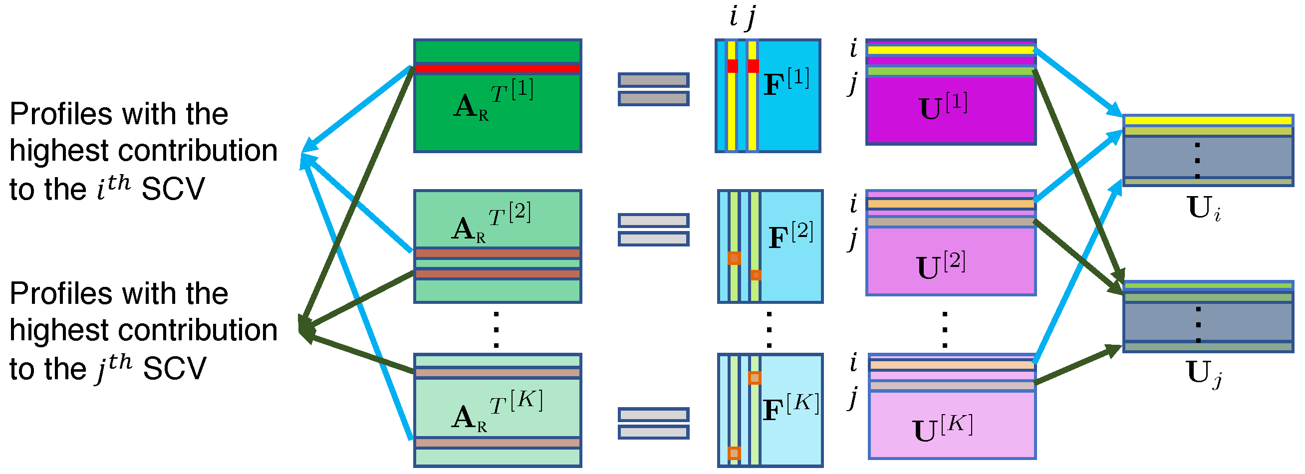
2.3.4. C-ICT Step 4: Tracing Back to Components

In the last stage, for each significantly correlated SCV, we identify K subject profiles with the highest contribution to that SCV from the K modalities, as shown in Figure 1c, and trace back to their corresponding ICs, as shown in Figure 1d. These ICs are defined as components that are associated across K modalities. The kth second-level source component in the c th SCV represents a linear combination of all rows of B [ k ] ; i.e., a linear combination of all columns of F [ k ] , where c = 1 , 2 , , C . In other words, the kth second-level component in the c th SCV is a linear combination of all subject covariations from the kth modalities, weighted by the coefficients in the cth column of the second-level mixing matrix F [ k ] . The cth column of the estimated second-level mixing matrices, F [ k ] , represents the weights of the subject covariations for the c th SCV. We identify the indices i [ k ] of the largest absolute value of the coefficient in the cth column of F [ k ] for the kth modality, respectively, implying the i [ k ] th row of F [ k ] has the highest contribution to the cth SCV. Then, the i [ 1 ] , i [ 2 ] , , i [ K ] th ICs that correspond to the i [ k ] th subject covariations obtained above are identified to be the cth associated ICs across K modalities.
Note that the back-reconstructed subject profiles are no longer necessarily orthogonal to each other from the same modality, so one subject profile might be dependent on multiple subject profiles from another modality. This enables C-ICT to be able to discover such “one-to-many associations” in this context; i.e., one IC from one modality may be associated with multiple ICs from another modality, which is a great advantage for the multimodal fusion method. The identification of “one-to-many associations” is illustrated in Figure 3. After identifying the associated subject profiles among K modalities, the ICs corresponding to these subject profiles are identified as associated among the K modalities; thus, the “one-to-many associations” are identified.

3. Implementation and Results

3.1. Implementation

To exclude non-brain voxels, we performed masking on the FA, GM, and fALFF data separately using the Group ICA of fMRI Toolbox (GIFT) [58]. A matrix of the FA dataset with dimensions of 162 × 49,277 (number of subjects × number of dMRI voxels) was constructed for the dMRI dataset. A matrix of the GM dataset with dimensions of 162 × 60,636 (number of subjects × number of sMRI voxels) was constructed for the sMRI dataset. A matrix of the fALFF dataset with dimensions of 162 × 69,519 (number of subjects × number of fMRI voxels) was constructed for the fMRI dataset. Then, we implemented the proposed framework C-ICT to fuse the three datasets to explore the multiple associations across the dMRI, sMRI, and fMRI modalities.

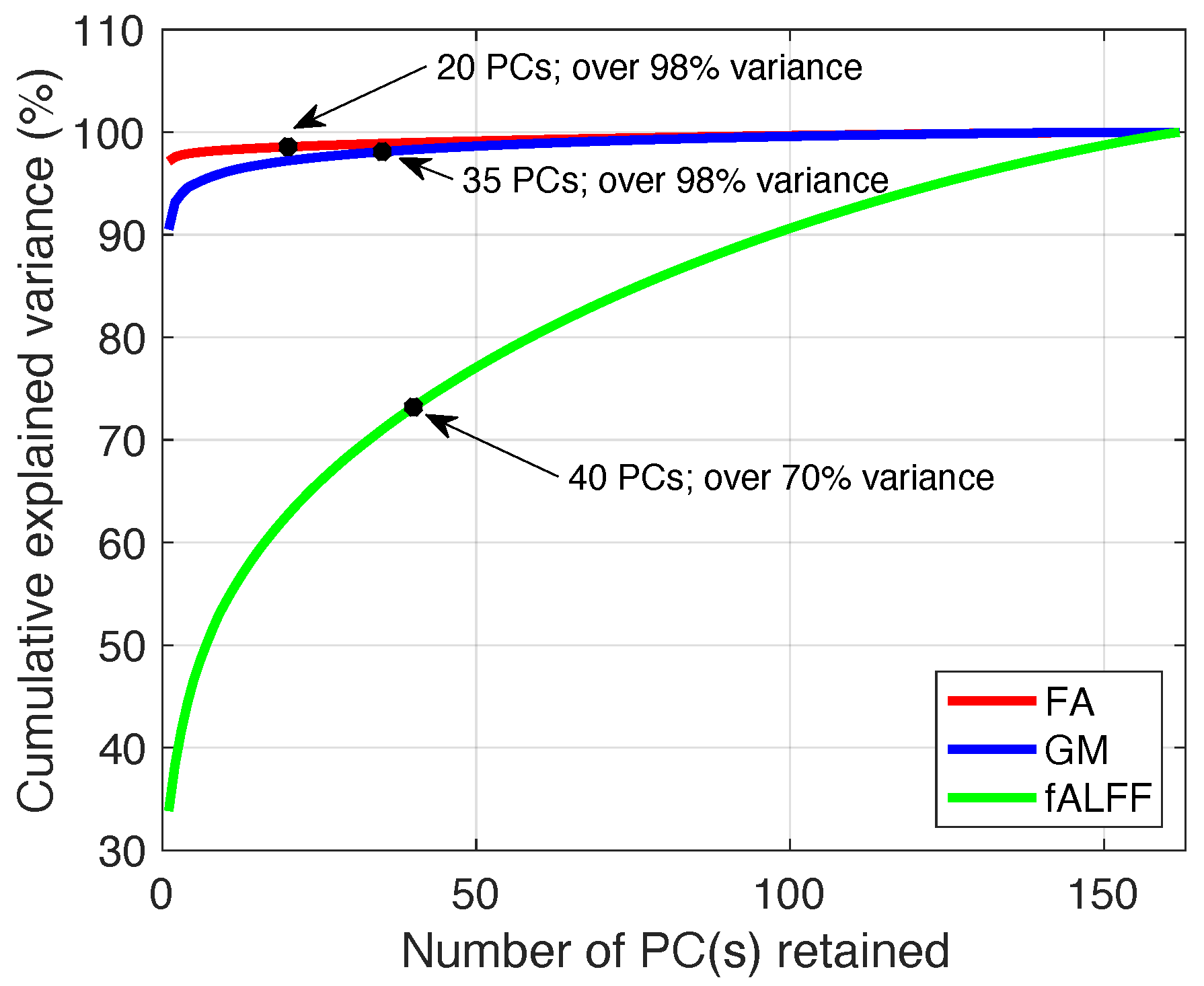
3.1.1. Order Selection

We performed PCA on each dataset separately and calculated the cumulative explained variance (shown in Figure 2). From Figure 2, we can see that the variance retained for the FA and GM datasets follows a similar pattern, which differs from that of the fALFF dataset. For this reason, the criteria for order selection were similar for the FA and GM datasets. We used 98% as the threshold for the variance retained for the FA and GM datasets in order to balance the retention of the most signal while minimizing the effects of noise. As a result, the orders used for FA and GM datasets were 20 and 35, respectively.
Using a similar threshold for the variance retained with the fALFF dataset would result in an order of 145. Model order that is greater than 100 has been found to decrease the stability of ICA [59]. Therefore, using a variance retained threshold is not an appropriate way to determine the order for the fALFF dataset as was done for the FA and GM datasets. Instead, we determined the order for the fALFF dataset by investigating the effect of different orders on the estimated ICs [12,60,61,62]. We performed ICA to estimate ICs starting at an order of 20 and increasing the order with increments of 5 until the order reached 70. These limits were selected to cover a large range of potential, yet still reasonable, values for the order. As we increased the order from 20 to 40, we observed increasing numbers of meaningful neuroanatomical and functional components. However, when increasing the order beyond 40, we found that components of interest became split into multiple spatial maps and the number of the noise components increased. For this reason, we selected an order of 40 for the fALFF dataset, resulting in over 70% retained variance.

3.1.2. Algorithm Choice

Infomax [63] is a widely used ICA algorithm, particularly in the field of biomedical imaging. It assumes that the underlying source component has a super-Gaussian distribution, which is a good model-match for the brain imaging signals [64]. Therefore, we used Infomax for the C-ICT model in this study.
Since ICA is an iterative algorithm, the optimization of ICA yields different solutions depending on the initialization. Therefore, we performed ICA for 30 independent runs with different random initializations and selected the most consistent run using a metric called cross inter-symbol interference (cross-ISI) [65]. Similarly, IVA-G is also an iterative algorithm, so we performed IVA-G 50 times independently and used cross-ISI to select the most consistent run.

3.1.3. Artifact Elimination

After the ICA step, we obtained 20, 35, and 40 ICs for the FA, GM, and fALFF datasets, respectively. For dMRI, we used the ICBM-DTI-81 white-matter labels atlas and JHU white-matter tractography atlas [66,67,68], provided in FSL (fsl.fmrib.ox.ac.uk/fsl/fslwiki/, accessed on 10 November 2019) to identify the WM tracts. For sMRI and fMRI, each IC was transformed into Z-scores to obtain the zero mean and unit variance, and the voxels with a Z-score greater than the threshold 2 ( | Z | 2 ) were converted from MNI coordinates to Talairach coordinates and entered into a database to assign anatomical and functional labels for the left and right hemispheres.
To remove artifacts caused by body movements such as breathing and heart beating, we eliminated ICs from the brain ventricles or areas where large blood vessels are located [69,70]. We also eliminated ICs that were spread across wide regions of the brain or at the edges of brain images to remove motion-related signals [57,71]. More specifically, for the FA, we removed the ICs with spotty, diffusely distributed patterns over most of the brain, which represented noise. For the sMRI, we removed the sinus susceptibility noise and WM components [72]. For the fMRI, we removed ICs that were located beyond the area of GM; e.g., ventricles, skull, and surrounding tissue, WM, frontal/sagittal sinus susceptibility noise, CSF, and motion artifacts with ring patterns [72,73,74,75,76,77]. As a result, 10, 27, and 17 ICs were retained for FA, GM, and fALFF datasets, respectively. Their corresponding subject covariations were formed into three reduced subject covariation matrices with sizes of 10 × 162 (FA), 17 × 162 (fALFF), and 27 × 162 (GM), which were then used in the IVA step. The spatial maps of the retained components were converted to Z-scores and thresholded at | Z | 2 (Figure 4, Figure 5 and Figure 6).

3.1.4. Group Differences
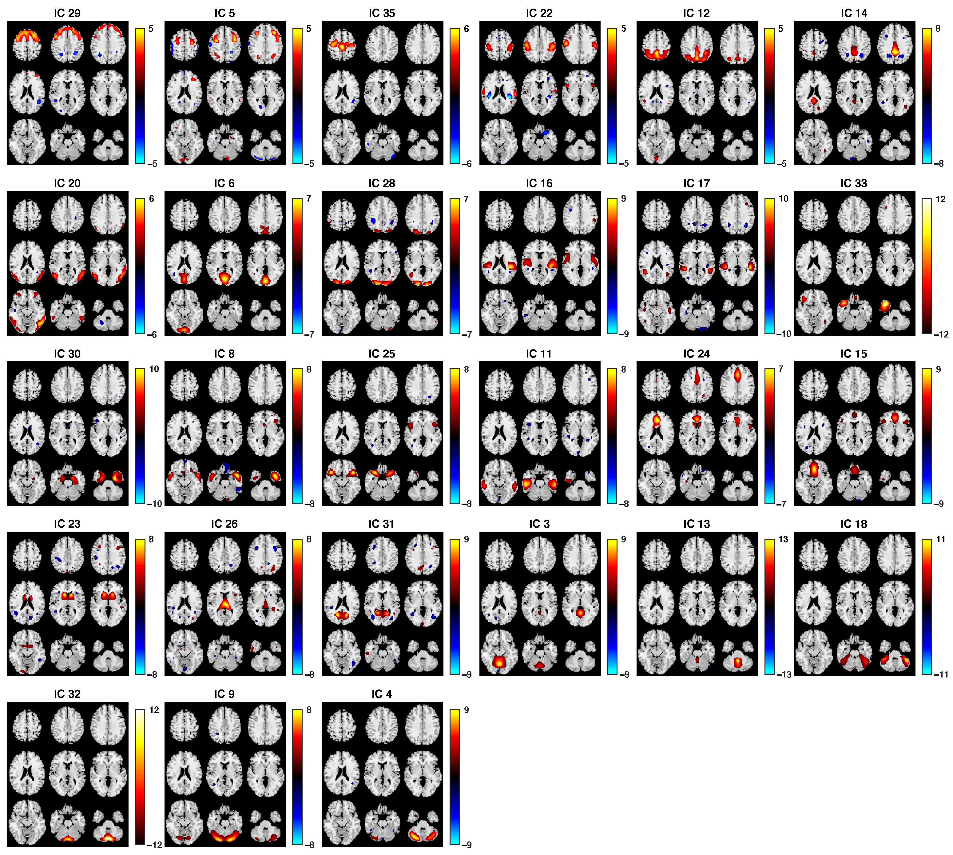
After identifying the associated ICs by performing the C-ICT on the three modalities, we performed a two-sample t-test on the corresponding subject covariations to identify ICs that showed a statistically significant difference between the two groups (HC vs. SZ; p < 0.05 ), which are referred to as biomarkers of schizophrenia. Associated IC triplets that showed significant group differences in all dMRI, sMRI and fMRI modalities are referred to as associated biomarkers of disease.

3.2. Fusion Results

Following the explained procedure, we discovered six IC linked triplets (Figure 7). The identified brain regions of each identified fALFF IC are summarized in Supplementary Table S1. Within each of the six triplets, three ICs that corresponded to three modalities (dMRI, sMRI and fMRI) were linked, representing a multimodal brain network with three nodes (WM, structural GM, and functional GM).
We found that the structure–structure associations were generally stronger than the structure–function associations (dMRI–sMRI: | ρ | = 0.48 ± 0.26 ; dMRI–fMRI: | ρ | = 0.32 ± 0.11 ; sMRI–fMRI: | ρ | = 0.33 ± 0.13 ; see Table 1). We also examined group differences (HC vs. SZ) for each IC on its corresponding subject covariation and found that more ICs showed significant group differences in sMRI than the other two modalities (5 in sMRI; 2 in dMRI; 1 in fMRI; p < 0.05; two-sample t-test; see Figure 7). Interestingly, for all these ICs in both the dMRI and the sMRI data that showed significant group differences, the SZ group showed less activation, suggesting both a reduced volume of the GM and reduced integrity of the WM in patients with SZ. For the ICs in fMRI that showed significant group differences, the SZ group had higher activation, perhaps suggesting less neural efficiency in patients with SZ.
We also note that one IC can be found in more than one triplet, meaning that one IC from one modality is associated with many ICs from other modalities. For instance, the IC (corticospinal tract and superior longitudinal fasciculus (CST-SLF)) from dMRI is not only associated with the uncus and inferior temporal gyrus (Uncus–ITG) from sMRI and superior frontal gyrus and middle frontal gyrus (SFG-MFG) from fMRI, but is also associated with the precuneus and paracentral lobule (Precuneus–PCL) from sMRI and superior temporal gyrus (STG) from fMRI, as shown in Figure 7 (green frame). Another shared IC between triplets is the postcentral gyrus and precentral gyrus (POG–PCG) from sMRI, which is not only associated with anterior thalamic radiation and the anterior corona radiata (ATR–ACR) from dMRI and thalamus from fMRI, but also associated with superior corona radiation and the corticospinal tract (SCR–CST) from dMRI and culmen from fMRI, as shown in Figure 7 (blue frame).

4. Discussion

In this study, we propose a new data fusion framework, C-ICT, to uncover relationships across multiple brain imaging modalities to reveal the underlying mechanisms of brain function as well as their dysfunction in diseases such as schizophrenia. Specifically, C-ICT uses ICA to extract independent brain networks from each modality and then explores possible associations across the modalities using IVA.
Compared with other existing data fusion frameworks, C-ICT is flexible in many ways. First, unlike jICA, mCCA + jICA, tIVA, and parallel ICA [15,25,26,27,78], C-ICT allows for different orders from the different datasets. Datasets of different modalities are different in nature and might also have different levels of signal-to-noise ratios (SNRs). Therefore, different orders would be expected for each modality. Second, C-ICT has no constraint on the number of datasets, like parallel ICA. This freedom is important because a greater number of data modalities can be collected from the same subjects. Thus, a framework that is capable of jointly analyzing all modalities at the same time can provide valuable insight into both the structural and functional aspects of networks responsible for brain functions. Third, C-ICT is unique in that it is able to discover “one-to-many associations” between datasets—a feature not available for any other data fusion method. This is possible for C-ICT because one IC with the highest contribution to one SCV might also have the highest contribution to other SCVs. The finding of such “one-to-many associations” suggests that one brain region can be recruited by multiple other regions for the performance of complex functions—an important neurobiological mechanism that is also supported by other studies [79,80,81]. In addition to being highly flexible, another advantage of the C-ICT framework is a critical step that eliminates ICs that might originate from artifacts such as heartbeats, respiratory movement, and non-brain signals. In doing so, we have observed more interpretable triplets of components, where each of the ICs from the three modalities are associated with each other, and stronger associations between modalities within each triplet, when compared with an implementation that skips this step.
We have applied the C-ICT framework to brain imaging data that measure structural and functional aspects of both the WM and GM through dMRI, sMRI, and fMRI in both HCs and SZs. As shown in the results, C-ICT uncovered six IC triplets. Importantly, within each triplet, the three associated components are observed to be all closely functionally related, thus validating our approach.
The first triplet includes anterior thalamic radiation and anterior corona radiata (ATR–ACR), postcentral gyrus and precentral gyrus (POG–PCG), and thalamus from dMRI, sMRI, and fMRI, respectively. The ATR is a WM bundle that connects the thalamus with the prefrontal cortex [82]. The thalamus is a hub that relays sensory information to the cerebral cortex [83]. The ACR carries somatotopically arranged motor fibers away from the cerebral cortex. The POG is where the primary somatosensory cortex is located, and PCG is where the primary motor cortex is located. This triplet represents a multimodal brain network that involves nodes that are all related to sensory–motor functions.
The second triplet includes the corpus callosum, superior temporal gyrus (STG), and paracentral lobule and postcentral gyrus (PCL–POG) from dMRI, sMRI, and fMRI, respectively. The corpus callosum is an important fiber bundle that connects the left and right brain hemispheres and allows communications of sensory, motor, and cognitive information between the two hemispheres. The STG is a cortical area responsible for auditory processing, multisensory integration, and spoken word recognition. The PCL is important for motor functions, while the POG is the location of the primary somatosensory cortex, which is responsible for the sense of touch. Thus, this triplet primarily focuses on sensory functions.
The third triplet includes the corticospinal tract and superior longitudinal fasciculus (CST–SLF), uncus and inferior temporal gyrus (Uncus–ITG), and superior frontal gyrus and middle frontal gyrus (SFG–MFG) from dMRI, sMRI, and fMRI, respectively. The CST is a fiber tract that originates from the motor-related cerebral cortex to the motor neurons and interneurons in the spinal cord and controls body movement. The SLF is a fiber tract that connects frontal, occipital, parietal, and temporal lobes including the premotor cortex, thus playing a role in regulating cognitive functions and motor behavior. The ITG is the anterior region of the temporal lobe, which is important for object cognition and memory. SFG and MFG occupy a large proportion of the frontal area that is also involved in cognition and motor functions. The three ICs within this triplet all show significant group differences between the HCs and SZs, suggesting that the structural and functional changes in these brain cognition and motor networks might be related to the cognitive dysfunction and motor deficits in SZs, thus revealing a multimodal neuroimaging biomarker of SZ.
The fourth triplet includes the superior longitudinal fasciculus (SLF), middle occipital gyrus and fusiform gyrus (MOG–FG), and cuneus and middle occipital gyrus (Cuneus–MOG) from dMRI, sMRI, and fMRI, respectively. The FG a large gyrus that spans across the temporal and occipital lobes. Both MOG and FG are involved in visual processing and cognition. Besides, the SLF is a fiber tract that connects to brain regions that are involved in cognitive function. Thus, this triplet might primarily process visual cognition such as object and facial recognition.
The fifth triplet includes CST–SLF, Precuneus–PCL, and STG from dMRI, sMRI, and fMRI, respectively. While both the structural components are involved in motor functions, the functional component is involved in sensory processing, representing a sensory–motor network across the three modalities. The sixth triplet includes SCR–CST, POG–PCG, and culmen from dMRI, sMRI, and fMRI, respectively. The three components are all related to motor function.
As we can see from the description of the six triplets, all triplets represent networks that are involved, at least partially, in motor functions, and many are related to cognitive functions. Importantly, we also find that the same IC appears in more than one triplet. Specifically, CST–SLF is in both triplet 3 (CST–SLF, Uncus–ITG, and SFG–MFG) and triplet 5 (CST–SLF, Precuneus–PCL, STG), and POG–PCG is in both triplet 1 (ATR–ACR, POG–PCG, and thalamus) and triplet 6 (SCR–CST, POG–PCG, and culmen), suggesting dual functions of one brain region in multiple multimodal brain networks.
Additionally, exploring the differences of ICs within the six triplets between HCs and SZs might provide information about potential biomarkers of schizophrenia. By using a two-sample t-test, we find that the ATR–ACR and CST–SLF from dMRI have stronger activation in HCs than in SZs, implying the WM in these regions is less integrated in SZs than in HCs. For sMRI, we find POG–PCG, STG, Uncus–ITG, and MOG–FG are less activated in SZs than in HCs, meaning that SZs have a reduced average GM volume in these areas. Furthermore, we find that SFG–MFG from fMRI has a stronger activation in SZs than HCs. Most of these regions has been reported to be associated with abnormalities and negative symptoms in SZs. SZs have been shown to have significantly lower FA values than HCs in the ATR [82,84,85,86], ACR [87], CST [88], and SLF regions [89]. In addition, the GM volume in the POG [90], PCG [91], STG [92], uncus [93], ITG [94,95], MOG [96], and FG [97] has been shown to be significantly decreased in SZs compared to in HCs.

5. Conclusions

It is increasingly common for multimodal data to be collected from the same subjects. This provides the motivation for the development of multimodal data fusion techniques, which have become important for the understanding of human brain imaging. In this paper, we proposed a novel multimodal data fusion framework, C-ICT, to explore multiple associations across different data modalities. We applied C-ICT to discover underlying relationships between dMRI, sMRI, and fMRI datasets from HCs and SZs. We have shown that C-ICT reveals multiple associations across the three modalities and provides potential biomarkers for schizophrenia, demonstrating that C-ICT is a flexible and informative method for the fusion of medical imaging data from different modalities. The success of C-ICT in this paper motivates its application to other modalities and domains. Besides the fusion of dMRI, sMRI, and fMRI data, C-ICT can be also used to fuse other types of multimodal data, such as magnetoencephalography (MEG) or genetic data. Moreover, this approach is not limited to the fusion of three data modalities but can be used for the fusion of many more modalities, thus enabling the discovery of more comprehensive associations across modalities in brain imaging studies as well as in other related areas.

Supplementary Materials

The following are available online at https://www.mdpi.com/article/10.3390/app11188382/s1, Table S1: Detailed information about the identified fALFF components.

Author Contributions

Conceptualization, C.J. and T.A.; Data curation, C.J. and V.D.C.; Formal analysis, C.J.; Funding acquisition, V.D.C. and T.A.; Investigation, C.J.; Methodology, C.J., M.A.B.S.A., Y.L.-S., Q.L. and T.A.; Project administration, T.A.; Resources, V.D.C. and T.A.; Software, C.J., M.A.B.S.A., Y.L.-S., Q.L. and T.A.; Supervision, T.A.; Validation, C.J.; Visualization, C.J. and T.A.; Writing—original draft, C.J.; Writing—review and editing, C.J., M.A.B.S.A., Y.L.-S., Q.L., V.D.C. and T.A. All authors have read and agreed to the published version of the manuscript.

Funding

This work was supported by the National Science Foundation (grants NSF-CCF 1618551, NSF-NCS 1631838) and National Institutes of Health grant R01-MH118695, R01-MH123610-01.

Institutional Review Board Statement

Not applicable.

Informed Consent Statement

Informed consent was obtained from all subjects involved in the study.

Data Availability Statement

The data used in this study are from the Center of Biomedical Research Excellence (COBRE), available from the Collaborative Informatics and Neuroimaging Suite data exchange repository [31,32] (coins.trendscenter.org/, accessed on 8 October 2018).

Acknowledgments

The authors would like to thank the research staff members from the Mind Research Network COBRE study for collecting, preprocessing, and sharing the data. The authors also appreciate the valuable feedback given by the members of Machine Learning for Signal Processing Laboratory at the University of Maryland, Baltimore County.

Conflicts of Interest

The authors declare no conflict of interest.

References

  1. Le Bihan, D.; Johansen-Berg, H. Diffusion MRI at 25: Exploring brain tissue structure and function. NeuroImage 2012, 61, 324–341. [Google Scholar] [CrossRef] [Green Version]
  2. Wang, Z.; Dai, Z.; Gong, G.; Zhou, C.; He, Y. Understanding structural-functional relationships in the human brain: A large-scale network perspective. Neuroscientist 2015, 21, 290–305. [Google Scholar] [CrossRef] [PubMed]
  3. Birur, B.; Kraguljac, N.V.; Shelton, R.C.; Lahti, A.C. Brain structure, function, and neurochemistry in schizophrenia and bipolar disorder—A systematic review of the magnetic resonance neuroimaging literature. NPJ Schizophr. 2017, 3, 1–15. [Google Scholar] [CrossRef]
  4. Dumoulin, S.O.; Fracasso, A.; van der Zwaag, W.; Siero, J.C.; Petridou, N. Ultra-high field MRI: Advancing systems neuroscience towards mesoscopic human brain function. NeuroImage 2018, 168, 345–357. [Google Scholar] [CrossRef]
  5. Le Bihan, D.; Mangin, J.F.; Poupon, C.; Clark, C.A.; Pappata, S.; Molko, N.; Chabriat, H. Diffusion tensor imaging: Concepts and applications. J. Magn. Reson. Imaging Off. J. Int. Soc. Magn. Reson. Med. 2001, 13, 534–546. [Google Scholar] [CrossRef]
  6. Coffman, J.A.; Bornstein, R.A.; Olson, S.C.; Schwarzkopf, S.B.; Nasrallah, H.A. Cognitive impairment and cerebral structure by MRI in bipolar disorder. Biol. Psychiatry 1990, 27, 1188–1196. [Google Scholar] [CrossRef]
  7. Biswal, B.; Zerrin Yetkin, F.; Haughton, V.M.; Hyde, J.S. Functional connectivity in the motor cortex of resting human brain using echo-planar MRI. Magn. Reson. Med. 1995, 34, 537–541. [Google Scholar] [CrossRef] [PubMed]
  8. Wang, S.; Fan, G. Alterations of structural and functional connectivity in profound sensorineural hearing loss infants within an early sensitive period: A combined DTI and fMRI study. Dev. Cogn. Neurosci. 2019, 38, 100654. [Google Scholar] [CrossRef]
  9. Hirjak, D.; Rashidi, M.; Kubera, K.M.; Northoff, G.; Fritze, S.; Schmitgen, M.M.; Sambataro, F.; Calhoun, V.D.; Wolf, R.C. Multimodal magnetic resonance imaging data fusion reveals distinct patterns of abnormal brain structure and function in catatonia. Schizophr. Bull. 2020, 46, 202–210. [Google Scholar] [CrossRef] [Green Version]
  10. Sui, J.; Yu, Q.; He, H.; Pearlson, G.; Calhoun, V.D. A selective review of multimodal fusion methods in schizophrenia. Front. Hum. Neurosci. 2012, 6, 27. [Google Scholar] [CrossRef] [PubMed] [Green Version]
  11. Lahat, D.; Adali, T.; Jutten, C. Multimodal data fusion: An overview of methods, challenges, and prospects. Proc. IEEE 2015, 103, 1449–1477. [Google Scholar] [CrossRef] [Green Version]
  12. Adali, T.; Levin-Schwartz, Y.; Calhoun, V.D. Multimodal data fusion using source separation: Application to medical imaging. Proc. IEEE 2015, 103, 1494–1506. [Google Scholar] [CrossRef]
  13. Calhoun, V.D.; Adali, T. Feature-based fusion of medical imaging data. IEEE Trans. Inf. Technol. Biomed. 2008, 13, 711–720. [Google Scholar] [CrossRef] [Green Version]
  14. James, A.P.; Dasarathy, B.V. Medical image fusion: A survey of the state of the art. Inf. Fusion 2014, 19, 4–19. [Google Scholar] [CrossRef] [Green Version]
  15. Adali, T.; Levin-Schwartz, Y.; Calhoun, V.D. Multimodal data fusion using source separation: Two effective models based on ICA and IVA and their properties. Proc. IEEE 2015, 103, 1478–1493. [Google Scholar] [CrossRef] [Green Version]
  16. Adali, T.; Akhonda, M.; Calhoun, V.D. ICA and IVA for data fusion: An overview and a new approach based on disjoint subspaces. IEEE Sens. Lett. 2018, 3, 1–4. [Google Scholar] [CrossRef] [PubMed]
  17. Comon, P.; Jutten, C. Handbook of Blind Source Separation: Independent Component Analysis and Applications; Academic Press: Cambridge, MA, USA, 2010. [Google Scholar]
  18. Harold, H. Relations between two sets of variates. Biometrika 1936, 28, 321–377. [Google Scholar]
  19. Correa, N.M.; Li, Y.O.; Adali, T.; Calhoun, V.D. Canonical correlation analysis for feature-based fusion of biomedical imaging modalities and its application to detection of associative networks in schizophrenia. IEEE J. Sel. Top. Signal Process. 2008, 2, 998–1007. [Google Scholar] [CrossRef] [PubMed] [Green Version]
  20. Kim, T.; Eltoft, T.; Lee, T.W. Independent vector analysis: An extension of ICA to multivariate components. In Proceedings of the International Conference on Independent Component Analysis and Signal Separation, Charleston, SC, USA, 5–8 March 2006; Springer: Berlin/Heidelberg, Germany, 2006; pp. 165–172. [Google Scholar]
  21. Adali, T.; Anderson, M.; Fu, G.S. Diversity in independent component and vector analyses: Identifiability, algorithms, and applications in medical imaging. IEEE Signal Process. Mag. 2014, 31, 18–33. [Google Scholar] [CrossRef]
  22. Kettenring, J.R. Canonical analysis of several sets of variables. Biometrika 1971, 58, 433–451. [Google Scholar] [CrossRef]
  23. Correa, N.M.; Eichele, T.; Adali, T.; Li, Y.; Calhoun, V.D. Multi-set canonical correlation analysis for the fusion of concurrent single trial ERP and functional MRI. NeuroImage 2010, 50, 1438–1445. [Google Scholar] [CrossRef] [Green Version]
  24. Anderson, M.; Fu, G.S.; Phlypo, R.; Adali, T. Independent vector analysis: Identification conditions and performance bounds. IEEE Trans. Signal Process. 2014, 62, 4399–4410. [Google Scholar] [CrossRef] [Green Version]
  25. Calhoun, V.D.; Adali, T.; Pearlson, G.; Kiehl, K.A. Neuronal chronometry of target detection: Fusion of hemodynamic and event-related potential data. NeuroImage 2006, 30, 544–553. [Google Scholar] [CrossRef] [PubMed]
  26. Sui, J.; He, H.; Pearlson, G.D.; Adali, T.; Kiehl, K.A.; Yu, Q.; Clark, V.P.; Castro, E.; White, T.; Mueller, B.A.; et al. Three-way (N-way) fusion of brain imaging data based on mCCA+ jICA and its application to discriminating schizophrenia. NeuroImage 2013, 66, 119–132. [Google Scholar] [CrossRef] [PubMed] [Green Version]
  27. Levin-Schwartz, Y.; Calhoun, V.D.; Adali, T. Data-driven fusion of EEG, functional and structural MRI: A comparison of two models. In Proceedings of the 2014 48th Annual Conference on Information Sciences and Systems (CISS), Princeton, NJ, USA, 19–21 March 2014; pp. 1–6. [Google Scholar]
  28. Akhonda, M.A.B.S.; Levin-Schwartz, Y.; Bhinge, S.; Calhoun, V.D.; Adali, T. Consecutive independence and correlation transform for multimodal fusion: Application to EEG and fMRI data. In Proceedings of the 2018 IEEE International Conference on Acoustics, Speech and Signal Processing (ICASSP), Calgary, AB, Canada, 15–20 April 2018; pp. 2311–2315. [Google Scholar]
  29. Jia, C.; Akhonda, M.A.B.S.; Long, Q.; Calhoun, V.D.; Waldstein, S.; Adali, T. C-ICT for Discovery of Multiple Associations in Multimodal Imaging Data: Application to Fusion of fMRI and DTI Data. In Proceedings of the 2019 53rd Annual Conference on Information Sciences and Systems (CISS), Baltimore, MD, USA, 20–22 March 2019; pp. 1–5. [Google Scholar]
  30. Anderson, M.; Adali, T.; Li, X.L. Joint blind source separation with multivariate Gaussian model: Algorithms and performance analysis. IEEE Trans. Signal Process. 2011, 60, 1672–1683. [Google Scholar] [CrossRef]
  31. Scott, A.; Courtney, W.; Wood, D.; De la Garza, R.; Lane, S.; Wang, R.; King, M.; Roberts, J.; Turner, J.A.; Calhoun, V.D. COINS: An innovative informatics and neuroimaging tool suite built for large heterogeneous datasets. Front. Neuroinform. 2011, 5, 33. [Google Scholar] [CrossRef] [Green Version]
  32. Wood, D.; King, M.; Landis, D.; Courtney, W.; Wang, R.; Kelly, R.; Turner, J.A.; Calhoun, V.D. Harnessing modern web application technology to create intuitive and efficient data visualization and sharing tools. Front. Neuroinform. 2014, 8, 71. [Google Scholar] [CrossRef] [PubMed]
  33. Bell, C.C. DSM-IV: Diagnostic and statistical manual of mental disorders. JAMA 1994, 272, 828–829. [Google Scholar] [CrossRef]
  34. Aine, C.; Bockholt, H.J.; Bustillo, J.R.; Cañive, J.M.; Caprihan, A.; Gasparovic, C.; Hanlon, F.M.; Houck, J.M.; Jung, R.E.; Lauriello, J.; et al. Multimodal neuroimaging in schizophrenia: Description and dissemination. Neuroinformatics 2017, 15, 343–364. [Google Scholar] [CrossRef]
  35. Jones, D.K.; Horsfield, M.A.; Simmons, A. Optimal strategies for measuring diffusion in anisotropic systems by magnetic resonance imaging. Magn. Reson. Med. Off. J. Int. Soc. Magn. Reson. Med. 1999, 42, 515–525. [Google Scholar] [CrossRef]
  36. Deichmann, R.; Gottfried, J.A.; Hutton, C.; Turner, R. Optimized EPI for fMRI studies of the orbitofrontal cortex. NeuroImage 2003, 19, 430–441. [Google Scholar] [CrossRef]
  37. Shin, J.; Ahn, S.; Hu, X. Correction for the T1 effect incorporating flip angle estimated by Kalman filter in cardiac-gated functional MRI. Magn. Reson. Med. 2013, 70, 1626–1633. [Google Scholar] [CrossRef] [Green Version]
  38. Assaf, Y.; Pasternak, O. Diffusion tensor imaging (DTI)-based white matter mapping in brain research: A review. J. Mol. Neurosci. 2008, 34, 51–61. [Google Scholar] [CrossRef]
  39. Van Erp, T.G.; Greve, D.N.; Rasmussen, J.; Turner, J.; Calhoun, V.D.; Young, S.; Mueller, B.; Brown, G.G.; McCarthy, G.; Glover, G.H.; et al. A multi-scanner study of subcortical brain volume abnormalities in schizophrenia. Psychiatry Res. Neuroimaging 2014, 222, 10–16. [Google Scholar] [CrossRef] [Green Version]
  40. Bockholt, H.J.; Scully, M.; Courtney, W.; Rachakonda, S.; Scott, A.; Caprihan, A.; Fries, J.; Kalyanam, R.; Segall, J.; De La Garza, R.; et al. Mining the mind research network: A novel framework for exploring large scale, heterogeneous translational neuroscience research data sources. Front. Neuroinform. 2010, 3, 36. [Google Scholar] [CrossRef] [PubMed] [Green Version]
  41. Freire, L.; Roche, A.; Mangin, J.F. What is the best similarity measure for motion correction in fMRI time series? IEEE Trans. Med. Imaging 2002, 21, 470–484. [Google Scholar] [CrossRef] [PubMed]
  42. Zou, Q.; Zhu, C.; Yang, Y.; Zuo, X.; Long, X.; Cao, Q.; Wang, Y.; Zang, Y. An improved approach to detection of amplitude of low-frequency fluctuation (ALFF) for resting-state fMRI: Fractional ALFF. J. Neurosci. Methods 2008, 172, 137–141. [Google Scholar] [CrossRef] [Green Version]
  43. Heni, M.; Kullmann, S.; Ketterer, C.; Guthoff, M.; Linder, K.; Wagner, R.; Stingl, K.; Veit, R.; Staiger, H.; Häring, H.U.; et al. Nasal insulin changes peripheral insulin sensitivity simultaneously with altered activity in homeostatic and reward-related human brain regions. Diabetologia 2012, 55, 1773–1782. [Google Scholar] [CrossRef] [PubMed] [Green Version]
  44. Tang, Y.Y.; Tang, R.; Posner, M.I. Brief meditation training induces smoking reduction. Proc. Natl. Acad. Sci. USA 2013, 110, 13971–13975. [Google Scholar] [CrossRef] [Green Version]
  45. Chen, A.C.; Oathes, D.J.; Chang, C.; Bradley, T.; Zhou, Z.W.; Williams, L.M.; Glover, G.H.; Deisseroth, K.; Etkin, A. Causal interactions between fronto-parietal central executive and default-mode networks in humans. Proc. Natl. Acad. Sci. USA 2013, 110, 19944–19949. [Google Scholar] [CrossRef] [Green Version]
  46. Wang, G.Z.; Belgard, T.G.; Mao, D.; Chen, L.; Berto, S.; Preuss, T.M.; Lu, H.; Geschwind, D.H.; Konopka, G. Correspondence between resting-state activity and brain gene expression. Neuron 2015, 88, 659–666. [Google Scholar] [CrossRef] [Green Version]
  47. Kong, F.; Hu, S.; Wang, X.; Song, Y.; Liu, J. Neural correlates of the happy life: The amplitude of spontaneous low frequency fluctuations predicts subjective well-being. Neuroimage 2015, 107, 136–145. [Google Scholar] [CrossRef] [PubMed]
  48. Holmes, A.J.; Hollinshead, M.O.; O’keefe, T.M.; Petrov, V.I.; Fariello, G.R.; Wald, L.L.; Fischl, B.; Rosen, B.R.; Mair, R.W.; Roffman, J.L.; et al. Brain Genomics Superstruct Project initial data release with structural, functional, and behavioral measures. Sci. Data 2015, 2, 1–16. [Google Scholar] [CrossRef] [Green Version]
  49. Turner, J.A.; Damaraju, E.; Van ERP, T.G.; Mathalon, D.H.; Ford, J.M.; Voyvodic, J.; Mueller, B.A.; Belger, A.; Bustillo, J.; McEwen, S.C.; et al. A multi-site resting state fMRI study on the amplitude of low frequency fluctuations in schizophrenia. Front. Neurosci. 2013, 7, 137. [Google Scholar] [CrossRef] [Green Version]
  50. Comon, P. Independent component analysis, a new concept? Signal Process. 1994, 36, 287–314. [Google Scholar] [CrossRef]
  51. Beckmann, C.F.; DeLuca, M.; Devlin, J.T.; Smith, S.M. Investigations into resting-state connectivity using independent component analysis. Philos. Trans. R. Soc. B Biol. Sci. 2005, 360, 1001–1013. [Google Scholar] [CrossRef] [PubMed] [Green Version]
  52. De Pasquale, F.; Della Penna, S.; Snyder, A.Z.; Lewis, C.; Mantini, D.; Marzetti, L.; Belardinelli, P.; Ciancetta, L.; Pizzella, V.; Romani, G.L.; et al. Temporal dynamics of spontaneous MEG activity in brain networks. Proc. Natl. Acad. Sci. USA 2010, 107, 6040–6045. [Google Scholar] [CrossRef] [PubMed] [Green Version]
  53. Calhoun, V.D.; Adali, T. Multisubject independent component analysis of fMRI: A decade of intrinsic networks, default mode, and neurodiagnostic discovery. IEEE Rev. Biomed. Eng. 2012, 5, 60–73. [Google Scholar] [CrossRef] [Green Version]
  54. Li, Y.O.; Yang, F.G.; Nguyen, C.T.; Cooper, S.R.; LaHue, S.C.; Venugopal, S.; Mukherjee, P. Independent component analysis of DTI reveals multivariate microstructural correlations of white matter in the human brain. Hum. Brain Mapp. 2012, 33, 1431–1451. [Google Scholar] [CrossRef] [PubMed]
  55. Long, Q.; Bhinge, S.; Calhoun, V.D.; Adali, T. Independent vector analysis for common subspace analysis: Application to multi-subject fMRI data yields meaningful subgroups of schizophrenia. NeuroImage 2020, 216, 116872. [Google Scholar] [CrossRef] [PubMed]
  56. McKeown, M.J.; Makeig, S.; Brown, G.G.; Jung, T.P.; Kindermann, S.S.; Bell, A.J.; Sejnowski, T.J. Analysis of fMRI data by blind separation into independent spatial components. Hum. Brain Mapp. 1998, 6, 160–188. [Google Scholar] [CrossRef]
  57. Beckmann, C.F. Modelling with independent components. NeuroImage 2012, 62, 891–901. [Google Scholar] [CrossRef] [PubMed]
  58. Calhoun, V.D.; Adali, T. Group ICA of fMRI Toolbox (GIFT). 2004. Available online: https://trendscenter.org/software/ (accessed on 23 February 2019).
  59. Abou-Elseoud, A.; Starck, T.; Remes, J.; Nikkinen, J.; Tervonen, O.; Kiviniemi, V. The effect of model order selection in group PICA. Hum. Brain Mapp. 2010, 31, 1207–1216. [Google Scholar] [CrossRef] [PubMed]
  60. Correa, N.M.; Adali, T.; Li, Y.; Calhoun, V.D. Canonical correlation analysis for data fusion and group inferences. IEEE Signal Process. Mag. 2010, 27, 39–50. [Google Scholar] [CrossRef] [Green Version]
  61. Chen, J.; Calhoun, V.D.; Liu, J. ICA order selection based on consistency: Application to genotype data. In Proceedings of the 2012 Annual International Conference of the IEEE Engineering in Medicine and Biology Society, San Diego, CA, USA, 28 August–1 September 2012; pp. 360–363. [Google Scholar]
  62. Laney, J.; Adali, T.; Waller, S.M.; Westlake, K.P. Quantifying motor recovery after stroke using independent vector analysis and graph-theoretical analysis. NeuroImage Clin. 2015, 8, 298–304. [Google Scholar] [CrossRef] [Green Version]
  63. Bell, A.J.; Sejnowski, T.J. An information-maximization approach to blind separation and blind deconvolution. Neural Comput. 1995, 7, 1129–1159. [Google Scholar] [CrossRef]
  64. Correa, N.M.; Adali, T.; Li, Y.; Calhoun, V.D. Comparison of blind source separation algorithms for fMRI using a new Matlab toolbox: GIFT. In Proceedings of the (ICASSP ’05), IEEE International Conference on Acoustics, Speech, and Signal Processing, Philadelphia, PA, USA, 23 March 2005; Volume 5, p. v-401. [Google Scholar]
  65. Long, Q.; Jia, C.; Boukouvalas, Z.; Gabrielson, B.; Emge, D.; Adali, T. Consistent run selection for independent component analysis: Application to fMRI analysis. In Proceedings of the 2018 IEEE International Conference on Acoustics, Speech and Signal Processing (ICASSP), Calgary, AB, Canada, 15–20 April 2018; pp. 2581–2585. [Google Scholar]
  66. Mori, S.; Wakana, S.; Van Zijl, P.C.; Nagae-Poetscher, L. MRI Atlas of Human White Matter; Elsevier: Amsterdam, The Netherlands, 2005. [Google Scholar]
  67. Wakana, S.; Caprihan, A.; Panzenboeck, M.M.; Fallon, J.H.; Perry, M.; Gollub, R.L.; Hua, K.; Zhang, J.; Jiang, H.; Dubey, P.; et al. Reproducibility of quantitative tractography methods applied to cerebral white matter. NeuroImage 2007, 36, 630–644. [Google Scholar] [CrossRef] [Green Version]
  68. Hua, K.; Zhang, J.; Wakana, S.; Jiang, H.; Li, X.; Reich, D.S.; Calabresi, P.A.; Pekar, J.J.; van Zijl, P.C.; Mori, S. Tract probability maps in stereotaxic spaces: Analyses of white matter anatomy and tract-specific quantification. NeuroImage 2008, 39, 336–347. [Google Scholar] [CrossRef] [Green Version]
  69. Kelly, R.E., Jr.; Alexopoulos, G.S.; Wang, Z.; Gunning, F.M.; Murphy, C.F.; Morimoto, S.S.; Kanellopoulos, D.; Jia, Z.; Lim, K.O.; Hoptman, M.J. Visual inspection of independent components: Defining a procedure for artifact removal from fMRI data. J. Neurosci. Methods 2010, 189, 233–245. [Google Scholar] [CrossRef] [PubMed] [Green Version]
  70. Calhoun, V.D.; Adali, T. Unmixing fMRI with independent component analysis. IEEE Eng. Med. Biol. Mag. 2006, 25, 79–90. [Google Scholar] [CrossRef]
  71. Ray, K.L.; McKay, D.R.; Fox, P.M.; Riedel, M.C.; Uecker, A.M.; Beckmann, C.F.; Smith, S.M.; Fox, P.T.; Laird, A. ICA model order selection of task co-activation networks. Front. Neurosci. 2013, 7, 237. [Google Scholar] [CrossRef] [Green Version]
  72. Feis, R.A.; Smith, S.M.; Filippini, N.; Douaud, G.; Dopper, E.G.; Heise, V.; Trachtenberg, A.J.; van Swieten, J.C.; van Buchem, M.A.; Rombouts, S.A.; et al. ICA-based artifact removal diminishes scan site differences in multi-center resting-state fMRI. Front. Neurosci. 2015, 9, 395. [Google Scholar] [CrossRef] [Green Version]
  73. Tohka, J.; Foerde, K.; Aron, A.R.; Tom, S.M.; Toga, A.W.; Poldrack, R.A. Automatic independent component labeling for artifact removal in fMRI. NeuroImage 2008, 39, 1227–1245. [Google Scholar] [CrossRef] [PubMed] [Green Version]
  74. Bhaganagarapu, K.; Jackson, G.D.; Abbott, D.F. An automated method for identifying artifact in independent component analysis of resting-state fMRI. Front. Hum. Neurosci. 2013, 7, 343. [Google Scholar] [CrossRef] [Green Version]
  75. Griffanti, L.; Douaud, G.; Bijsterbosch, J.; Evangelisti, S.; Alfaro-Almagro, F.; Glasser, M.F.; Duff, E.P.; Fitzgibbon, S.; Westphal, R.; Carone, D.; et al. Hand classification of fMRI ICA noise components. NeuroImage 2017, 154, 188–205. [Google Scholar] [CrossRef]
  76. Power, J.D.; Plitt, M.; Laumann, T.O.; Martin, A. Sources and implications of whole-brain fMRI signals in humans. NeuroImage 2017, 146, 609–625. [Google Scholar] [CrossRef] [PubMed] [Green Version]
  77. Kassinopoulos, M.; Mitsis, G.D. Identification of physiological response functions to correct for fluctuations in resting-state fMRI related to heart rate and respiration. NeuroImage 2019, 202, 116150. [Google Scholar] [CrossRef] [PubMed]
  78. Liu, J.; Pearlson, G.; Windemuth, A.; Ruano, G.; Perrone-Bizzozero, N.I.; Calhoun, V.D. Combining fMRI and SNP data to investigate connections between brain function and genetics using parallel ICA. Hum. Brain Mapp. 2009, 30, 241–255. [Google Scholar] [CrossRef] [PubMed] [Green Version]
  79. Bressler, S.L.; Menon, V. Large-scale brain networks in cognition: Emerging methods and principles. Trends Cogn. Sci. 2010, 14, 277–290. [Google Scholar] [CrossRef]
  80. Pessoa, L. Understanding brain networks and brain organization. Phys. Life Rev. 2014, 11, 400–435. [Google Scholar] [CrossRef] [Green Version]
  81. Hwang, K.; Bertolero, M.A.; Liu, W.B.; D’esposito, M. The human thalamus is an integrative hub for functional brain networks. J. Neurosci. 2017, 37, 5594–5607. [Google Scholar] [CrossRef] [PubMed] [Green Version]
  82. Young, K.A.; Manaye, K.F.; Liang, C.L.; Hicks, P.B.; German, D.C. Reduced number of mediodorsal and anterior thalamic neurons in schizophrenia. Biol. Psychiatry 2000, 47, 944–953. [Google Scholar] [CrossRef]
  83. Sherman, S.M.; Guillery, R.W. Exploring the Thalamus and Its Role in Cortical Function; MIT Press: Cambridge, MA, USA, 2006. [Google Scholar]
  84. McIntosh, A.M.; Maniega, S.M.; Lymer, G.K.S.; McKirdy, J.; Hall, J.; Sussmann, J.E.; Bastin, M.E.; Clayden, J.D.; Johnstone, E.C.; Lawrie, S.M. White matter tractography in bipolar disorder and schizophrenia. Biol. Psychiatry 2008, 64, 1088–1092. [Google Scholar] [CrossRef] [PubMed]
  85. Mamah, D.; Conturo, T.E.; Harms, M.P.; Akbudak, E.; Wang, L.; McMichael, A.R.; Gado, M.H.; Barch, D.M.; Csernansky, J.G. Anterior thalamic radiation integrity in schizophrenia: A diffusion-tensor imaging study. Psychiatry Res. Neuroimaging 2010, 183, 144–150. [Google Scholar] [CrossRef] [PubMed] [Green Version]
  86. Ćurčić-Blake, B.; Nanetti, L.; van der Meer, L.; Cerliani, L.; Renken, R.; Pijnenborg, G.H.; Aleman, A. Not on speaking terms: Hallucinations and structural network disconnectivity in schizophrenia. Brain Struct. Funct. 2015, 220, 407–418. [Google Scholar] [CrossRef] [PubMed]
  87. Koshiyama, D.; Fukunaga, M.; Okada, N.; Morita, K.; Nemoto, K.; Yamashita, F.; Yamamori, H.; Yasuda, Y.; Fujimoto, M.; Kelly, S.; et al. Role of frontal white matter and corpus callosum on social function in schizophrenia. Schizophr. Res. 2018, 202, 180–187. [Google Scholar] [CrossRef] [PubMed]
  88. Epstein, K.A.; Cullen, K.R.; Mueller, B.A.; Robinson, P.; Lee, S.; Kumra, S. White matter abnormalities and cognitive impairment in early-onset schizophrenia-spectrum disorders. J. Am. Acad. Child Adolesc. Psychiatry 2014, 53, 362–372. [Google Scholar] [CrossRef] [Green Version]
  89. Karlsgodt, K.H.; van ERP, T.G.; Poldrack, R.A.; Bearden, C.E.; Nuechterlein, K.H.; Cannon, T.D. Diffusion tensor imaging of the superior longitudinal fasciculus and working memory in recent-onset schizophrenia. Biol. Psychiatry 2008, 63, 512–518. [Google Scholar] [CrossRef]
  90. Glahn, D.C.; Laird, A.R.; Ellison-Wright, I.; Thelen, S.M.; Robinson, J.L.; Lancaster, J.L.; Bullmore, E.; Fox, P.T. Meta-analysis of gray matter anomalies in schizophrenia: Application of anatomic likelihood estimation and network analysis. Biol. Psychiatry 2008, 64, 774–781. [Google Scholar] [CrossRef] [Green Version]
  91. Zhou, S.Y.; Suzuki, M.; Hagino, H.; Takahashi, T.; Kawasaki, Y.; Matsui, M.; Seto, H.; Kurachi, M. Volumetric analysis of sulci/gyri-defined in vivo frontal lobe regions in schizophrenia: Precentral gyrus, cingulate gyrus, and prefrontal region. Psychiatry Res. Neuroimaging 2005, 139, 127–139. [Google Scholar] [CrossRef]
  92. Barta, P.E.; Pearlson, G.D.; Powers, R.E.; Richards, S.S.; Tune, L.E. Auditory hallucinations and smaller superior temporal gyral volume in schizophrenia. Am. J. Psychiatry 1990, 147, 1457–1462. [Google Scholar]
  93. Job, D.E.; Whalley, H.C.; McConnell, S.; Glabus, M.; Johnstone, E.C.; Lawrie, S.M. Structural gray matter differences between first-episode schizophrenics and normal controls using voxel-based morphometry. NeuroImage 2002, 17, 880–889. [Google Scholar] [CrossRef] [PubMed]
  94. Onitsuka, T.; Shenton, M.E.; Salisbury, D.F.; Dickey, C.C.; Kasai, K.; Toner, S.K.; Frumin, M.; Kikinis, R.; Jolesz, F.A.; McCarley, R.W. Middle and inferior temporal gyrus gray matter volume abnormalities in chronic schizophrenia: An MRI study. Am. J. Psychiatry 2004, 161, 1603–1611. [Google Scholar] [CrossRef]
  95. Kuroki, N.; Shenton, M.E.; Salisbury, D.F.; Hirayasu, Y.; Onitsuka, T.; Ersner, H.; Yurgelun-Todd, D.; Kikinis, R.; Jolesz, F.A.; McCarley, R.W. Middle and inferior temporal gyrus gray matter volume abnormalities in first-episode schizophrenia: An MRI study. Am. J. Psychiatry 2006, 163, 2103–2110. [Google Scholar] [CrossRef] [Green Version]
  96. Cascella, N.G.; Fieldstone, S.C.; Rao, V.A.; Pearlson, G.D.; Sawa, A.; Schretlen, D.J. Gray-matter abnormalities in deficit schizophrenia. Schizophr. Res. 2010, 120, 63–70. [Google Scholar] [CrossRef] [PubMed]
  97. Onitsuka, T.; Shenton, M.E.; Kasai, K.; Nestor, P.G.; Toner, S.K.; Kikinis, R.; Jolesz, F.A.; McCarley, R.W. Fusiform gyrus volume reduction and facial recognition in chronic schizophrenia. Arch. Gen. Psychiatry 2003, 60, 349–355. [Google Scholar] [CrossRef] [PubMed]
Figure 1. Flowchart of C-ICT. (a) Perform ICA on each dataset separately to obtain subject covariation matrices and ICs. (b) Eliminate subject covariations corresponding to artifact components. (c) Apply IVA-G on the reduced subject covariation matrices to obtain SCVs and the second-level mixing matrices. SCVs that show significant pair-wise correlation are chosen for further analysis. (d) Subject covariations with the highest contribution to the correlated SCVs chosen above are identified and their corresponding ICs are identified as the associated components across K modalities. The first SCV is highlighted for clarity. The same color of the bars in the different matrices denotes the same index in the corresponding rows and columns.
Applsci 11 08382 g001
Figure 2. Cumulative explained variance accounting for different PCs from the FA, GM, and fALFF datasets. For each dataset, the black point on the curve indicates the variance explained by the number of PCs we selected.
Applsci 11 08382 g002
Figure 3. Identification of “one-to-many associations”. In the first modality, the indices of the largest absolute value of the coefficient in the ith column and the jth column of F [ 1 ] are the same, meaning that the same subject profile (marked in red) makes the highest contribution to the ith SCV and the jth SCV. This subject profile from the first modality is associated with the two subject profiles from the second modality and two subject profiles from the Kth modality.
Applsci 11 08382 g003
Figure 4. Spatial maps of 10 retained ICs from the FA dataset. These results reflect the IC results of SZ and HC groups combined. The brain maps are visualized at | Z | 2 , with positive Z values in red color and negative Z values in blue.
Applsci 11 08382 g004
Figure 5. Spatial maps of 27 retained ICs from the GM dataset. These results reflect the IC results of SZ and HC groups combined. The brain maps are visualized at | Z | 2 , with positive Z values in red color and negative Z values in blue.
Applsci 11 08382 g005
Figure 6. Spatial maps of 17 retained ICs from the fALFF dataset. These results reflect the IC results of SZ and HC groups combined. The brain maps are visualized at | Z | 2 , with positive Z values in red color and negative Z values in blue.
Applsci 11 08382 g006
Figure 7. Summary of the six IC linked triplets. The spatial maps of all ICs were converted to Z-scores and thresholded by | Z | 2 . Each row shows the three associated ICs from dMRI, sMRI, and fMRI, respectively. The abbreviations of brain regions identified by ICs are shown above the spatial maps. If one IC shows a statistically significant activation between HCs and SZs ( p < 0.05 ; t-test), the p value would be shown above the map, where the red color indicates higher activation in HCs than patients and the blue color indicates lower activation in HCs than patients. Note that the IC 7 (green frame) from dMRI is associated with two ICs from sMRI and two ICs from fMRI. IC 22 (blue frame) from sMRI is associated with two ICs from dMRI and two ICs from fMRI.
Applsci 11 08382 g007
Table 1. The absolute values of the pair-wise Pearson correlation coefficients | ρ | corresponding to the associated triplets and the values of p ρ .
Triplet #dMRI–sMRIdMRI–fMRIsMRI–fMRI
1 | ρ | = 0.80 , p ρ = 4 × 10 37 | ρ | = 0.27 , p ρ = 5.6 × 10 4 | ρ | = 0.49 , p ρ = 3.6 × 10 1
2 | ρ | = 0.67 , p ρ = 4.2 × 10 22 | ρ | = 0.43 , p ρ = 1.2 × 10 8 | ρ | = 0.38 , p ρ = 1.9 × 10 4
3 | ρ | = 0.62 , p ρ = 1.8 × 10 18 | ρ | = 0.32 , p ρ = 3.8 × 10 5 | ρ | = 0.21 , p ρ = 4 × 10 3
4 | ρ | = 0.43 , p ρ = 1.6 × 10 8 | ρ | = 0.21 , p ρ = 7.7 × 10 3 | ρ | = 0.2 , p ρ = 1.2 × 10 2
5 | ρ | = 0.18 , p ρ = 2.6 × 10 2 | ρ | = 0.21 , p ρ = 6.9 × 10 3 | ρ | = 0.43 , p ρ = 8.4 × 10 9
6 | ρ | = 0.18 , p ρ = 2 × 10 2 | ρ | = 0.46 , p ρ = 1.1 × 10 9 | ρ | = 0.25 , p ρ = 1.2 × 10 3
Publisher’s Note: MDPI stays neutral with regard to jurisdictional claims in published maps and institutional affiliations.

